The Distribution Dynamics of Carbon Dioxide Emissions Intensity across Chinese Provinces: A Weighted Approach

Abstract

This paper examines the distribution dynamics of carbon dioxide (CO₂) emissions intensity across 30 Chinese provinces using a weighted distribution dynamics approach. The results show that CO₂ emissions intensity tends to diverge during the sample period of 1995–2014. However, convergence clubs are found in the ergodic distributions of the full sample and two sub-sample periods. Divergence, polarization, and stratification are the dominant characteristics in the distribution dynamics. Weightings with economic and population sizes have important impacts on current distributions and hence long-run steady distributions. Neglecting the size of the economy may underestimate the deterioration in the long-run steady state. The result also shows that conditioning on space and income cannot eliminate the multimodality in the long-run distribution. However, capital intensity has an important impact on the formation of convergence clubs. Our findings will contribute to an understanding of the spatial dynamic behaviors of CO₂ emissions across Chinese provinces, and have important policy implications for CO₂ emissions reduction in China.

1. Introduction

Under threat of global warming, CO₂ emissions abatement has become one of the most important environmental concerns during the past decades. In 2007 China surpassed the United States to become the world’s largest CO₂ emitter. The huge amount and rapid growth of CO₂ emissions in China have attracted considerable attention from both policy-makers and researchers. Moreover, after decades of rapid economic growth, income growth has been accompanied by serious environmental deterioration. Obviously, the development model of the past decades is not sustainable and requires transformation and upgrading. The Chinese government is facing the problems of environmental degradation and international pressure to reduce CO₂ emissions, and has taken actions to reduce CO₂ emissions in recent development plans. For example, in the 2009 Copenhagen conference, the Chinese government pledged a CO₂ emissions intensity (the ratio of CO₂ emissions over GDP) reduction of 40%–45% from 2005 to 2020. In 2014, the government further promised to reach its carbon emissions peak before 2030.

Understanding the transitional dynamics and long-term trend of CO₂ emissions is important for achieving greenhouse gas reduction. The convergence of CO₂ emissions is a core concern of policy-makers. In China, the national CO₂ emission reduction target is disaggregated on the provincial level in terms of emissions intensity. The convergence of CO₂ emissions across provinces is expected and implies equity in CO₂ abatement. Moreover, if the convergence is achieved without policy intervention, as indicated by the Environmental Kuznets Curve (EKC) paradigm, this implies that high emitters may reduce their emissions as the economy develops. On the contrary, lack of convergence in CO₂ emissions may suggest inequity in CO₂ abatement and cause damage to the credibility of local and national government in their efforts to reduce CO₂ emissions. Moreover, it may also suggest a lack of technology diffusion across provinces.

The concept of convergence is derived from the neo-classical growth theory, which indicates that poor countries will catch up with rich countries due to diminished returns for capital. There are generally three types of convergence, namely σ-convergence, β-convergence, and stochastic convergence, which are most popularly tested in empirical studies. In terms of CO₂ emissions, σ-convergence measures the dispersion changes in CO₂ emission level over time. β-convergence implies the negative relationship between the initial CO₂ emission level and subsequent growth rate, while stochastic convergence implies that the CO₂ emission level in a region is relative to that of the economy as a whole and has a stationary trend. However, a negative coefficient between the initial CO₂ emissions level and subsequent growth is a necessary but not sufficient condition for convergence. Thus the distribution dynamics approach suggests investigating the evolutionary trend of the variable in question. Thus the distribution dynamics use more information to measure the dynamic behavior of CO₂ emissions level across regions. It can be taken as an upgraded examination of convergence.

There are already some studies that focus on the convergence behavior of CO₂ emissions across provinces in China [1,2,3,4,5]. However, due to differences in emission variables (per capita CO₂ emissions or emissions intensity), sample periods, and econometric approaches, the empirical results in the existing literature remain inherently controversial. For example, Wang et al. found evidence of divergence in CO₂ emissions intensity [3], while many others found evidence of convergence in per capita CO₂ emissions [1,2] and emissions intensity [4,5]. These studies use traditional approaches to examine the convergence in terms of per capita CO₂ emissions or emissions intensity. However, these traditional approaches, such as σ-convergence, β-convergence, and stochastic convergence, are based on models for average or representative economies, which help us understand the evolution of CO₂ emissions in general but provide little information for the distribution dynamics of CO₂ emissions across provinces [6]. In addition, these approaches provide no information on the entire shape of the distribution and intra-distribution mobility, namely the relative position changes in terms of CO₂ emissions. Finally, Chinese provinces differ greatly in terms of economy and population size. For example, the economy and population of Guangdong, a southern province in China, are 43 and 16 times those of Ninxia Province, one of the northwestern Chinese provinces, respectively. The welfare effect of a one percent reduction in CO₂ emissions in Guangdong is much different from that in Ninxia. To the best of our knowledge, no study has yet examined the importance of the economy and population size in the convergence analysis of CO₂ emissions.

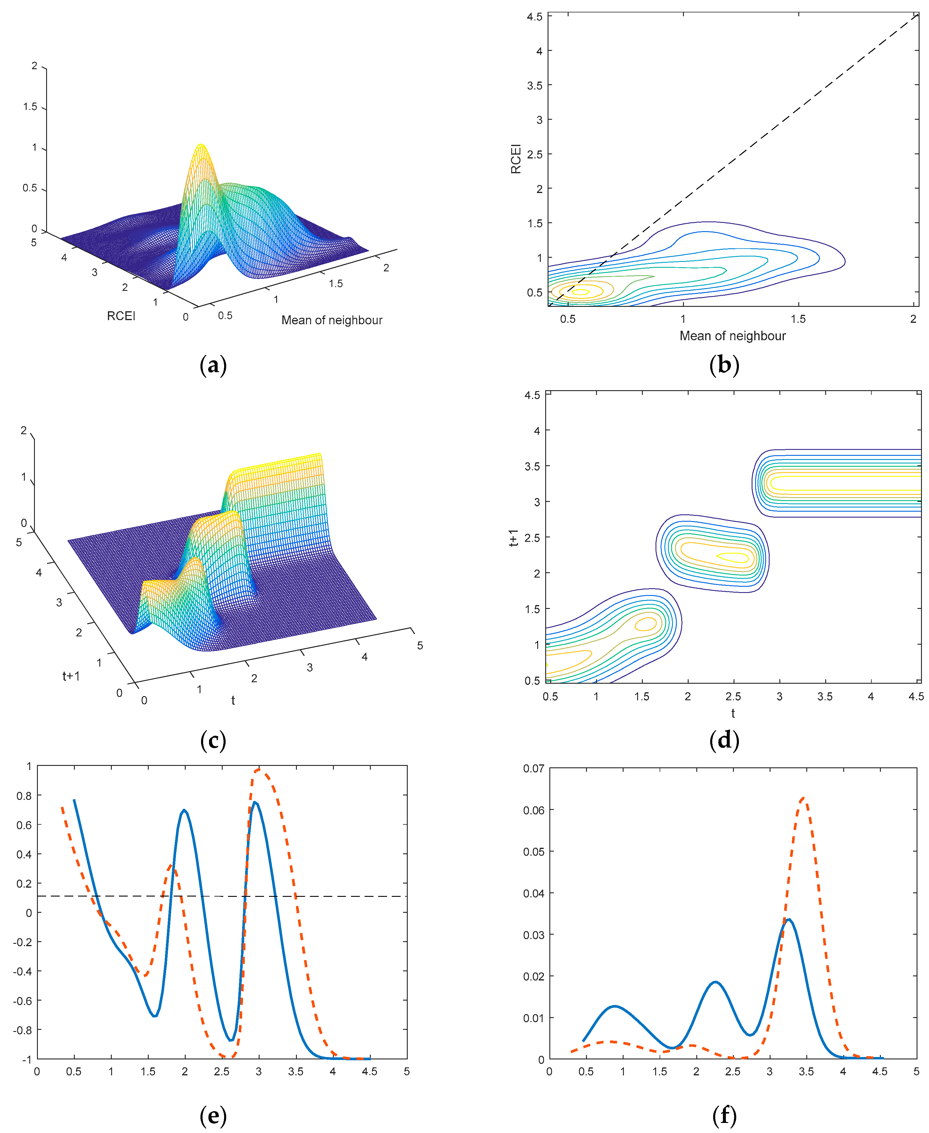
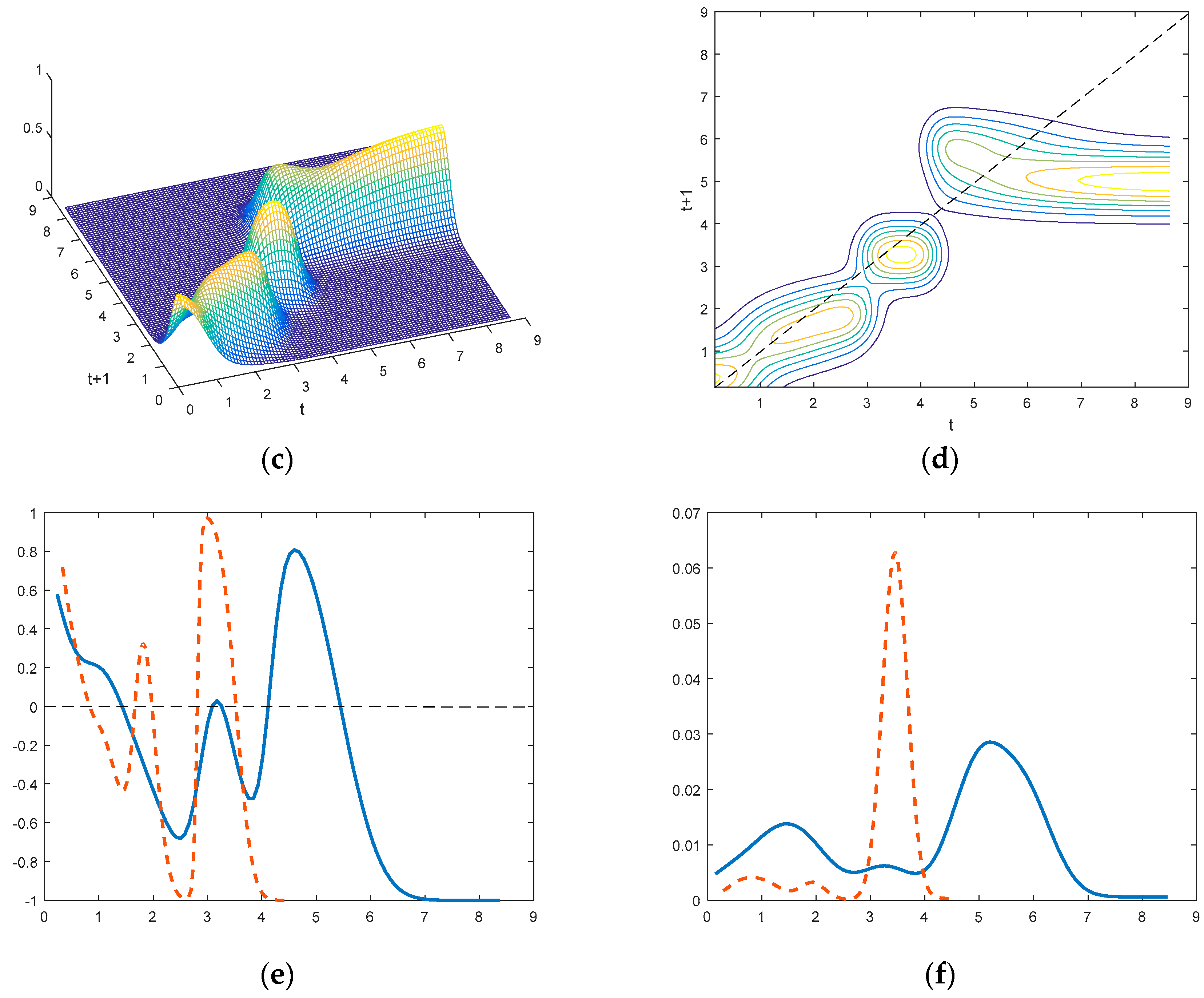
This paper, therefore, aims to investigate the spatial distribution dynamics of CO₂ emissions intensity across 30 Chinese provinces. Our analysis differs from those in the existing literature in several aspects: First, we adopt a continuous dynamic distribution approach to examine the dynamic behavior of CO₂ emissions in China. The advantage of this approach is that it can provide a dynamic law for the entire shape of the distribution for CO₂ emissions across provinces. For example, it can provide detailed information about persistence, stratification, and polarization in the distribution dynamic process. Moreover, we use a net transition probability approach to provide more accurate measurements for convergence. Second, the impact of economic and population sizes are considered in the analysis, which is important in policy-making in China. Third, this paper also explores the factors that may influence the distribution dynamics of CO₂ emissions intensity in China using a combination of a joint distribution approach and a conditional distribution approach. This further provides information on the formation of convergence clubs.

This paper uses CO₂ emissions intensity instead of per capita CO₂ emissions in the analysis. Focusing on CO₂ emissions intensity has several advantages. First, as a developing country, achieving economic growth and environmental protection are both goals for China in the long run. CO₂ emissions intensity is a better indicator of the trade-off between economic growth and environmental protection than per capita CO₂ emissions. It encourages both economic growth and CO₂ emissions reduction in the production process. Second, CO₂ emissions reduction targets in China are based on emissions intensity rather than per capita emissions. Thus an examination of the distribution dynamics of CO₂ emissions intensity will have important policy implications. For example, regions with high emissions intensity and an increasing tendency in their relative emissions intensity should have more stringent regulations imposed on them than regions with low emissions intensity. Finally, emissions intensity can be taken as a measure of emissions efficiency and technology to some degree. Thus the convergence in CO₂ emissions intensity may suggest the existence of technology spillover and a catch-up effect among Chinese regions. Encouraging technology spillover and efficiency improvement are the most cost-effective ways to achieve sustainable development targets in China.

The remainder of this paper is organized as follows. Section 2 presents a review of the related literature. Section 3 presents the methodology. Section 4 describes the data. Section 5 presents the empirical results and discussions. Section 6 further examines the determinants of the distribution dynamics using a conditional distribution approach. Section 7 provides concluding remarks and discussions of policy implications.

2. Literature Review

With the increasing concern about global climate change, whether CO₂ emissions converge or diverge attracts much attention from researchers. However, what is the mechanism behind the convergence in CO₂ emissions? Many studies examine the possible existence of an inverted U-shaped relationship known as an Environmental Kuznets Curve (EKC) between economic development and environmental pollution (including CO₂ emissions). The rationale behind the EKC is complicated in terms of underlying driving forces. Improvement in technology and energy efficiency, increased environmental awareness, and enforcement of environmental regulations are forces that may reduce environmental pollution [7]. Supposing that EKC exists, it is easy to conclude that CO₂ emissions would converge over time. In the current literature, many theoretical models try to explain the mechanisms behind EKC [7,8,9].

The empirical research on the convergence of CO₂ emissions focuses heavily on both the international level across nations and the regional level within a specific country. Strazicich and List first examine the convergence behavior of CO₂ emissions across countries [10]. They investigate both stochastic and conditional convergences of per capita CO₂ emissions across 21 industrial countries using panel unit root tests and cross-sectional regressions. They find evidence for convergence in these industrial countries. Following this work, a growing body of literature examined the convergence of CO₂ emissions across countries using different sampling and estimation approaches. The first strand of literature uses traditional parametric approaches [11,12,13,14,15,16,17,18,19]. This strand of literature examines the existence of absolute, conditional, and stochastic convergence. However, the estimation results are sensitive to the choice of econometric approaches and datasets [17]. Moreover, the traditional approaches only provide limited information on the convergence. For example, β-convergence shows what happens to its mean, while σ-convergence only indicates the dispersion. The second strand of literature adopts nonparametric approaches [20,21,22,23,24,25]. Compared with the first strand of literature, the second strand of literature not only provides information for the convergence, but also highlights the dynamic law of the entire distribution shape for CO₂ emissions across countries, in particular the existence and formation of convergence clubs.

The huge amount of CO₂ emissions in China has also attracted a great deal of attention in recent years. Huang and Meng examine the convergence of per capita CO₂ emissions in urban China using a parametric model with spatial–temporal specifications [1]. Their results show evidence of convergence for the period 1985–2008. Using the log t test, Wang et al. found evidence for divergence at the country level and three convergence clubs in terms of CO₂ emissions intensity for the period 1996–2011 [3]. Wang and Zhang studied the β-convergence, stochastic convergence, and sigma convergence of per capita CO₂ emissions in six sectors across 28 provinces in China for the period 1996–2010 [2]. Their results indicated convergence in all sectors across the provinces. Hao et al. examined the convergence of CO₂ emissions intensity with provincial data for the period 1995–2011. They verified stochastic convergence and β-convergence among Chinese provincial samples [4]. Using a spatial dynamic panel data model, Zhao et al. examined the convergence of CO₂ emissions intensity across 30 provinces for the period 1990–2010. Their results supported the existence of convergence in CO₂ emissions intensity [5]. Instead of per capita CO₂ emissions and CO₂ emissions intensity, Li and Lin examined the convergence of energy efficiency with CO₂ emissions with provincial panel data [26].

The conclusions of existing studies on the convergence of CO₂ emissions in China are diverse due to the different estimation approaches and samples. As mentioned previously, the traditional convergence approaches have many limitations in estimating the spatial dynamic behavior of CO₂ emission distribution across countries or regions. They provide no information on the intra-distribution dynamics, which may be valuable both theoretically and empirically. For example, multimodality found in the long-run steady state may imply the existence of multiple equilibria in the evolution of CO₂ emissions. Therefore, instead of a single mechanism of the EKC, models of multiple equilibria are expected to shed light.

3. Research Method

3.1. Weighted Distribution Dynamics Approach

The distribution dynamics approach was developed by Danny Quah in a series of papers examining the evolution of income distribution across countries [27,28,29]. In comparison to the traditional parametric approaches, the distribution dynamics approach has several advantages. First, it provides more insights on the law of motion in an entire distribution of the variable in question, particularly in the formation of convergence clubs. Second, this approach is completely data-driven, and imposes no assumptions on the model, which helps avoid the estimation bias due to model assumption in parametric approaches. Third, this approach provides the possibility to account for economic and population sizes in the convergence analysis.

Let us suppose that cross-province distribution of CO₂ emissions intensity x at time t can be described by the density function ${\phi }_t\left(x\right)$. The evolution of the distribution is time-invariant and first-order, that is, the current distribution ${\phi }_t\left(x\right)$ at time t will evolve into the future distribution ${\phi }_{t+\tau }\left(y\right)$ at time t + τ, where τ > 0. Hence the relationship between the current distribution ${\phi }_t\left(x\right)$ and the future distribution ${\phi }_{t+\tau }\left(y\right)$ can be described as follows:

$${\phi }_{t+\tau }\left(y\right)={{\displaystyle \int }}_0^{\infty }{g}_{\tau }(y|x){\phi }_t\left(x\right)dx,$$

(1)

where $g_{\tau }(y|x)$ is the conditional density function that maps the transition process of the distribution of CO₂ emissions intensity. Keeping the conditional density function $g_{\tau }(y|x)$ unchanged, the distribution of CO₂ emissions intensity will evolve into a long-run equilibrium state, namely, the ergodic distribution. Therefore, the ergodic distribution ${\phi }_{\infty }\left(y\right)$ can be estimated as follows:

$${\phi }_{\infty }\left(y\right)={{\displaystyle \int }}_0^{\infty }{g}_{\tau }(y|x){\phi }_{\infty }\left(x\right)dx.$$

(2)

To understand the distribution dynamics of CO₂ emissions intensity, we need to know both the transition dynamics described by $g_{\tau }(y|x)$ and the long-run equilibrium distribution ${\phi }_{\infty }\left(y\right)$. For this purpose, a kernel density approach is used to estimate the conditional density function. The joint natural kernel estimator of ${\phi }_{t,t+\tau }\left(y,\mathrm{x}\right)$ and the marginal kernel estimator of ${\phi }_t\left(\mathrm{x}\right)$ can be defined as follows:

$${\phi }_{t,t+\tau }\left(y,\mathrm{x}\right)=\frac{1}{n{h}_x{h}_y}{\displaystyle \sum }_{i=1}^{n}K(\frac{x-x_i}{h_x},\frac{y-y_i}{h_y})$$

(3)

$${\phi }_t\left(\mathrm{x}\right)=\frac{1}{n{h}_x}{{\displaystyle \sum }}_{i=1}^{n}K(\frac{x-x_i}{h_x}),$$

(4)

where $x_i$ is the value of CO₂ emissions intensity in a specific province at time t, and $y_i$ is the value of CO₂ emissions intensity of that province at t + τ. We use $K(·)$ to denote kernel function. $h_x$ and $h_y$ denote the bandwidth of x and y, respectively. In this paper, the bandwidths are estimated using the method proposed by Silverman [30].

With these definitions, we can further estimate the conditional density with ${\phi }_{t,t+\tau }\left(y,\mathrm{x}\right)$ and ${\phi }_t\left(\mathrm{x}\right)$ through:

$$g_{\tau }\left(y|x\right)=\frac{{\phi }_{t,t+\tau }\left(y,x\right)}{{\phi }_t\left(x\right)}.$$

(5)

In order to account for economy or population sizes, we use population or economy sizes (the share of population or GDP) as weights in the analysis. The weighted kernel density can be estimated as follows:

$${\widehat{\phi }}_t\left(\mathrm{x}\right)=\frac{1}{n{h}_x}{{\displaystyle \sum }}_{i=1}^n{\omega }_i{K}_x(\frac{x-x_i}{h_x}),$$

(6)

where ${\omega }_i$ is the share of GDP or population in province i. In this paper, we give both unweighted and weighted analyses to provide full information on the distribution dynamics of CO₂ emissions intensity for Chinese provinces.

In the discrete approach, the transition dynamics is presented with a transition probability matrix. However, in the continuous approach, three-dimensional and contour plots are the most popular tools to show estimated results of transition probability. The three-dimensional plot can show the entire shape of the transition probability distribution, while a contour plot has the advantage of showing the deviation from the diagonal. Sometimes we need to know the net mobility tendency at each point. To gain more insight into the transition probability mass, we estimate the net transition probability (NTP) values at each point, which is an important index of mobility. The net transition probability index, denoted by $p\left(x\right)$, can be defined as:

$$p\left(x\right)={{\displaystyle \int }}_x^{\infty }{g}_{\tau }(z|x)dz-{{\displaystyle \int }}_0^x{g}_{\tau }(z|x)dz.$$

(7)

According to this definition, a positive net transition probability value at a point indicates an increasing trend in CO₂ emissions intensity, while a negative net transition probability value at a point implies a decreasing trend. Following common practice in dynamic distribution approaches, we use relative CO₂ emissions intensity (RCEI), which is the individual province’s CO₂ emissions intensity divided by its yearly average. Therefore, the RCEI values of a specific province correspond to the times of the CO₂ emissions intensity for this province relative to the provincial average.

3.2. Joint Distribution and Conditional Distribution Approach

Traditional convergence analysis always examines the convergence clubs with arbitrarily classified regional groups. However, spatial proximity is only one possible reason behind convergence clubs. Other factors, such as income level and capital intensity, may also affect the formation of convergence clubs. Therefore, new approaches are required to account for the formation of convergence clubs. This paper thereby adopts the joint distribution approach and the conditional distribution approach to investigate the determinants of the distribution. The joint distribution approach shows the joint kernel density distribution of RCEI and explanatory variables of interest, such as relative income or relative capital. The estimation is similar to that in Equation (3).

In the conditional distribution approach, we need to pre-filter the data to take out the influence of the conditioning variables before the analysis. Specifically, the spatial-conditional RCEI is the RCEI of a province relative to the average of its geographical neighbors. The income and capital intensity conditional RCEI are RCEI divided by relative income and capital intensity, respectively. For this reason, the conditional distribution RCEI can be interpreted as the part unexplained by the variable in question. The greater the difference between the distributions of the unconditional and conditional RCEIs, the greater the explanatory power of the variable in question.

4. Data

There were 34 provincial level administration units in China, namely 22 provinces, five autonomous regions, four municipalities, and three special administration regions (i.e., Hong Kong, Macau, and Taiwan). For simplicity, we use the concept of provinces to denote all the provincial administration units. Due to the data availability, we use a panel dataset across 30 provinces (without Hong Kong, Macau, Taiwan, and Tibet) from 1995 to 2014. Our panel data are drawn from official publications of the Chinese statistical agency. The three major sources are the China Energy Statistical Yearbook (CESY, various years), China Compendium of Statistics 1949–2008 (CCS), and China Statistical Yearbook (CSY, various years) [31,32,33].

4.1. CO₂ Emissions

The data for CO₂ emissions are not directly available at the provincial level in China. As CO₂ emissions are generated by the consumption of energy in provinces, we therefore estimate provincial CO₂ emissions based on energy consumption. We account for eight primary sources of energy consumptions and CO₂ emissions, namely coal, crude oil, coke, gasoline, kerosene, diesel oil, fuel oil, and natural gas. The formula to estimate CO₂ emissions is given by:

$$C{O}_2={{\displaystyle \sum }}_{i=1}^n{E}_i\times C{F}_i\times C{C}_i\times CO{F}_i\times \frac{44}{12},$$

(8)

where i indicates the categories of energy; $E_i$, $C{F}_i$, $C{C}_i$, and COF_i denote the consumption of energy, the transformation factor, the carbon emissions factor, and the carbon oxidation factor, respectively. The estimation is based on the criteria published by the Intergovernmental Panel on Climate Change (IPCC) (2006) [34]. Data for energy consumption in each province can be directly obtained from the annual China Energy Statistical Yearbook [31].

4.2. Population, GDP, and Capital

Our main source for the nominal GDP and population data used in this paper is the China Compendium of Statistics 1949–2008, and data after 2008 are from the China Statistic Yearbook (various years) [32,33]. The capital data are constructed using the same approach as in Wu [35]. The GDP and capital are deflated to the constant price of 1995.

5. Empirical Results

5.1. Preliminary Analysis

5.1.1. The Analysis of Dispersion

The coefficient of variation is always used as an indicator of dispersion in convergence analysis. Chinese provinces differ greatly in factor endowment, economic structure, climate, and regional development strategies. Interregional disparity in CO₂ emissions is one of the important components of difference in provincial CO₂ emissions. Following most studies, we classify Chinese provinces into three regions, namely the eastern, central, and western regions. Figure 1 shows the evolution trend of coefficient of variation and interregional ratios in terms of CO₂ emissions intensity for the period 1995–2014. We can observe that the coefficient of variation has a broadly increasing trend in most years. However, there are two sub-periods, namely 1999–2002, and 2008–2014, when the dispersion in terms of CO₂ emissions intensity increased sharply. The former is driven by the initiation of the Western Development Program, while the latter is driven by industry relocation policy in recent years. During the sample period, the ratio of central/east maintains a relatively steady state, while the ratio of west/east keeps an increasing trend. Moreover, the evolution trend of ratio of west/east is quite similar to that of the coefficient of variation. This may imply that the increase of dispersion is mainly driven by the diversion of CO₂ emissions intensity in the western region from the other two regions. This further proves that regional preferential policy has a significant impact on the spatial distribution of CO₂ emissions.

5.1.2. Analysis of the Distributions in Critical Years

The coefficient of variation can only provide information on the dispersion of CO₂ emissions intensity across provinces. To get more information about the entire shape of the spatial distribution, Figure 2 plots the unweighted kernel density distribution of RCEI in three representative years, namely, 1995, 2005, and 2014. All three distributions show significant multimodality, with a major peak below mean RCEI, and several small peaks in the high RCEI end. Moreover, all three distributions are significantly right-skewed. This indicates that most provinces are concentrated in the region below the mean RCEI values; only a small number of provinces are located in the high RCEI end. The major peak in the distribution increases over time in our sample period. However, the distribution of RCEI shrinks slightly at both ends for the period 1995–2005, while it increases significantly at the high end for the period 2005–2014. This suggests a divergence of CO₂ emissions intensity across the Chinese provinces, which is consistent with the results of coefficient of variation. Moreover, in comparison to the distribution in 1995, the distribution in 2014 shows more polarization and stratification.

As indicated in the previous section, Chinese provinces differ greatly in terms of economy and population size, which may have significant impacts on CO₂ emissions. Figure 3 shows the economic- and population-weighted distribution in three representative years. In all the three years’ distributions, all economic- and population-weighted distributions shrink the small peaks in the high RCEI end, but increase the major peak in the low RCEI end. However, weighting by economy size shifts the distribution more to the low RCEI than weighting by population size. This indicates that provinces with high CO₂ emissions intensity tend to have smaller economies and population sizes, while provinces with low CO₂ emissions intensity tend to have larger sizes. Therefore, neglecting economy and population size may bias the estimation of the real distribution of CO₂ emissions intensity across Chinese provinces. For example, Ninxia, which is the second smallest province in terms of both economy and population (second only to Tibet), has the highest CO₂ emissions intensity, while Guangdong, which is the largest in terms of both economy and population size, has the lowest CO₂ emissions intensity.

5.2. Distribution Dynamics in Chinese Provinces

5.2.1. The Full Sample

Figure 4 shows the distribution dynamics of RCEI for the period 1995–2014 with annual transitions. The three-dimensional plot in Figure 4a shows the distribution of the transitional probability mass with which a region with a specific RCEI value at time t could evolve into each value of RCEI at time t + 1, while the contour plot in Figure 4b is a top down view of the three-dimensional plot. To interpret this graph, suppose we choose a specific point (RCEI value of 2 for example) on the axis marked t, and then slice the plot from this point parallel to axis marked t + 1; this slice shows the probability distribution of a province with an RCEI value of 2 transitioning into each value of RCEI at time t + 1. In both plots, the concentration of probability mass along the diagonal implies higher persistence and immobility in relative position changes among provinces, while a deviation from the diagonal implies higher mobility in relative positions. In comparison with a three-dimensional plot, the contour plot shows the deviation from the diagonal line more clearly. Moreover, distinct peaks along the diagonal imply the existence of convergence clubs.

The three-dimensional plot in Figure 4a shows three peaks along the diagonal, implying the existence of convergence clubs in the long-run distribution. The contour plot in Figure 4b shows the deviation of transition probability mass from the diagonal line. It is observed that the transition probability mass is distributed along the diagonal in the low RCEI end, but there are more deviations from the diagonal line in the high RCEI end. This indicates higher persistence in the provinces with low RCEI values, while there is relatively high mobility among provinces with high RCEI values.

Net transition probability can provide more accurate information on the convergence of RCEI among provinces. Suppose that low-RCEI provinces have positive net transition probability, while high RCEI provinces have negative net transition probabilities; this will imply strong convergence in RCEI. Figure 4c shows the net transition probability for RCEI of Chinese provinces. Three regions, namely those with RCEI values less than 0.85, [1.65, 1.98], and [2.8, 3.5], have positive net transition probability, implying that provinces with RCEI values in these regions have a tendency to increase their CO₂ emissions intensity. From the policy perspective, these provinces should have more stringent CO₂ reduction targets imposed. Considering that the net transition probability is much higher in regions with an RCEI value of around 3, the central government should pay more attention to provinces with three times the average CO₂ emissions intensity. Differing from some existing studies [4,5], our results indicate divergence rather than convergence in CO₂ emissions intensity across Chinese provinces.

Figure 4d presents the ergodic distribution of RCEI based on the transition dynamics of RCEI for the period 1995–2014. Multimodality can be observed in the long-run steady distribution, with one major peak around the RCEI value of 3.5, and two small peaks around RCEI values of 1 and 2. Keeping the transition dynamics unchanged, Chinese provinces will converge into three clubs differentiated according to their CO₂ emissions intensity levels in the long run. This result is similar to that of Wang et al., who also find three convergence clubs among Chinese provinces [3]. Moreover, the ergodic distribution is heavily left-skewed, which differs greatly from the current distribution in Figure 2. The ergodic distribution has important implications for policy-making: the stratification of provinces in terms of CO₂ emissions intensity suggests that the government should take policy measures, such as encouraging interregional technology spillover and assigning tougher reduction targets to those provinces clustering into high RCEI clubs, to promote convergence among provinces.

As indicated in the previous section, neglecting province heterogeneity may bias the estimation of welfare effect in some cases. Figure 4e,f shows the weighted versions of net transition probability plot and ergodic distribution plot. For comparison, the unweighted curves are also included in the plots. In Figure 4e, weighting by economy and population size reduces the net transition probability for RCEI values less than 2, but increases net transition probability in regions with an RCEI value greater than 2. Moreover, weighting by economy size reduces the net transition probability more in the low-RCEI end than weighting by population size. Correspondingly, Figure 4f shows that weighting by economy and population size does not change the multimodality in the ergodic distribution, but significantly reduces the small peaks in the low-RCEI end while increasing the major peak in the high-RCEI end. This indicates that some relatively larger provinces tend to converge into high CO₂ emissions intensity club in the long run.

5.2.2. Distribution Dynamics in Two Sub-Periods

Before 2005, the Chinese government did not impose tight regulations on CO₂ emissions. However, facing serious environmental deterioration and international pressure, the Chinese government imposed stringent energy consumption and CO₂ emissions intensity targets in the 11th and 12th Five Year Plans (2005–2010 and 2011–2016, respectively). These policy changes may have impacted distribution dynamics before and after 2005. Therefore, the analysis is further conducted on two sub-periods, namely 1995–2005 and 2005–2014.

Figure 5 shows the distribution dynamics of RCEI with annul transition for the sub-period 1995–2005. Panels (a) and (b) show the unweighted three-dimensional and contour plots of transition probability mass distribution, while panels (c) and (d) show the net transition probability and the ergodic distribution plots. Although some small differences can be observed in the shapes of the distributions for transition probability compared with those in Figure 4, the distribution of transition probability mass in Figure 5 is generally similar to that in Figure 4. The ergodic distribution of unweighted RCEI for the period 1995–2005 (the solid line in Figure 5d) is significantly multimodal, with two large peaks around the RCEI value of 0.8 and 2, and a small peak around the RCEI value of 3.5. The three peaks in the ergodic distribution for the period 1995–2005 are more symmetrical than those for the full sample period. Compared with the current distribution for 1995 in Figure 2, a considerable number of provinces have a tendency to shift to the high CO₂ emissions intensity end. Moreover, weighting by economy and population size significantly increases the peaks around RCEI values of 0.8 and 3.5, but reduces the peak around the RCEI value of 2. Weighting by economy size has more impact on the ergodic distribution than weighting by population size. This implies that Chinese provinces have more disparity in economy size than in population size.

Figure 6 shows the distribution dynamics for RCEI across Chinese provinces with annual transitions for the sub-period 2005–2014. The distributions of transition probability mass in Figure 6a,b are significantly different from those in Figure 5. This implies that the transitional dynamics of RCEI in the sub-period 1995–2005 is different from that in the sub-period 2005–2014. The net transition probability curve in Figure 6c also exhibits some differences from that in Figure 5. There is only one region around the RCEI value of 2.8 that has positive net transition probability in the above-average region. Significant multimodality, with two small peaks around the RCEI value of 0.8 and 2, and a large peak around the RCEI value of 3.1, can be observed in the long-run distribution in Figure 6d. Compared with the right-skewed ergodic distribution in the sub-period 1995–2005, the ergodic distribution in the sub-period 2005–2014 is significantly left-skewed. If the distribution dynamics were kept unchanged in this sub-period, more provinces would converge into the high CO₂ emissions intensity clubs. In comparison to that in the sub-period 1995–2005, this implies more serious deterioration in the intra-distribution dynamics of RCEI in the sub-period 2005–2014. However, weighting by economy and population size has almost an opposite effect on the ergodic distribution in this sub-period. Weighting by economy size reduces the peaks in the low-RCEI end, but increases the peak in the high-RCEI end. On the contrary, weighting by population size increases the peaks in the low-RCEI end, but reduces the peak in the high end. This may imply that provinces with a larger economy tend to shift to the high-RCEI end more than average, while provinces with a larger population size have fewer tendencies to shift up.

6. The Determinants of Spatial Distribution Dynamics

Most studies on the convergence of CO₂ emissions only focus on the convergence itself. Few studies try to examine what factors affect the distribution dynamics of CO₂ emissions. Different from existing studies, this paper uses a new framework to analyze how geographical location, income level, and capital accumulation influence the distributional dynamics of RCEI with pre-filtered data. For simplicity, we only consider the unweighted analysis in this section.

6.1. The Dynamics of Spatial Conditional CO₂ Emissions Intensity

The joint distribution approach means that if the RCEI value of a specific province is close to its neighbor’s mean value, then the joint probability mass should distribute along the diagonal line. However, the three-dimensional plot (Figure 7a) and contour plot (Figure 7b) show that the joint probability mass deviates significantly from the diagonal line. This indicates that spatial location is not a significant factor in the formation of convergence clubs.

Figure 7 also shows the distribution dynamics of space conditional RCEI with annual transitions for the period 1995–2014. As a comparison, we also include the unconditional curves in the net transitional plot (Figure 7e) and ergodic distribution plot (Figure 7f). The three-dimensional plot (Figure 7c), contour plot (Figure 7d), and net transitional probability plot (Figure 7e) show that the transition dynamics of the space-conditional RCEI exhibits some differences to those in the unconditional case in Figure 4. More importantly, multimodality still exists in the ergodic distribution of space conditional RCEI. Conditioning on neighbor’s mean value does not eliminate convergence clubs in the long-run steady state. The distribution of conditional RCEI can be considered as the part unexplained by the variable in question. Hence, the above result indicates that the convergence clubs in the ergodic distribution of RCEI cannot be explained by geographical proximity. This result differs from that in Wang et al. [2], who found regional convergence clubs with a parametric approach. However, the parametric approach only provides the statistic result of “representative economy”. It is much less discriminating in finding the determinants of convergence clubs. Our result is more intuitive with more details than in previous studies.

6.2. The Dynamics of Income Conditional CO₂ Emissions Intensity

As discussed previously, income level is an important factor that may influence CO₂ emissions. The inverted U-shaped relationship between CO₂ emissions and income level, known as the “environmental Kuznets curve” (EKC), has been well documented in many studies. However, Bassetti et al. indicate that the nexus of income level and CO₂ emissions may be more complex than that predicted by the EKC paradigm [36]. For convenience, this paper employs relative income (RI) normalized to the yearly average in the analysis.

Figure 8a,b shows three-dimensional and contour plots of the joint distribution between RCEI and RI. It is observed that the probability mass distributes along two axes. Although most provinces are located in the highest peak in low income and low CO₂ emissions intensity regions, there is still a considerable number of provinces concentrated in the peaks along the two axes. “Low income, high pollution” provinces co-exist with “high income, low pollution” ones in China. This phenomenon cannot be explained by the EKC theory.

Figure 8c,d shows the distributions of transition probability mass for income-conditional RCEI with annual transitions for the period 1995–2014. There are some differences in the distribution of transition probability between the income-conditional RCEI in Figure 8 and the unconditional one in Figure 4. The net transition probability curve of conditional RCEI (the solid line in Figure 8e) also differs from that of unconditional RCEI (the dashed line in Figure 8e). Conditioning on income shows that income may have some impact on the distribution dynamics of CO₂ emissions intensity. However, the multimodality can still be observed in the ergodic distribution of income-conditional RCEI (the solid line in Figure 8f). Conditioning on income cannot eliminate the convergence clubs observed in the unconditional distribution.

6.3. The Distribution Dynamics of Capital Conditional CO₂ Emissions Intensity

High capital intensity is always related with high energy consumption and hence high CO₂ emissions. In this subsection, we focus on the relationship between CO₂ emissions intensity and capital intensity using a joint distribution approach and a conditional approach. Figure 9a,b shows the joint distribution of RCEI and relative capital (RK). As most of the density is concentrated in the below average area, no simple relationship can be observed in the joint distribution.

Figure 9c,d shows the distribution of transition probability mass for capital conditional RCEI with annual transitions for the period 1995–2014. In comparison with the unconditional case in Figure 4, the distribution dynamics of capital conditional RCEI differs from the unconditional one. The ergodic distribution for the conditional RCEI is bimodality, which is different from the multimodality of unconditional RCEI. The highest peak in the ergodic distribution disappears and the density mass is concentrated around the average. This indicates that capital intensity is an important factor in the formation of convergence clubs, the high CO₂ emissions intensity club in particular. These results have important policy implications. In China, the government plays an important role in capital investment. Hence, the government can promote convergence in CO₂ emissions intensity through capital investment policy.

7. Conclusions and Policy Implications

This paper examines the distribution dynamics of CO₂ emissions intensity across 30 provinces for the period 1995–2014. Different from existing studies, this paper adopts a weighted distribution dynamics approach, accounting for both economy and population size. Moreover, we use a combination of a joint distribution approach and a conditional distribution approach to examine the determinants of the distribution dynamics of CO₂ emissions intensity.

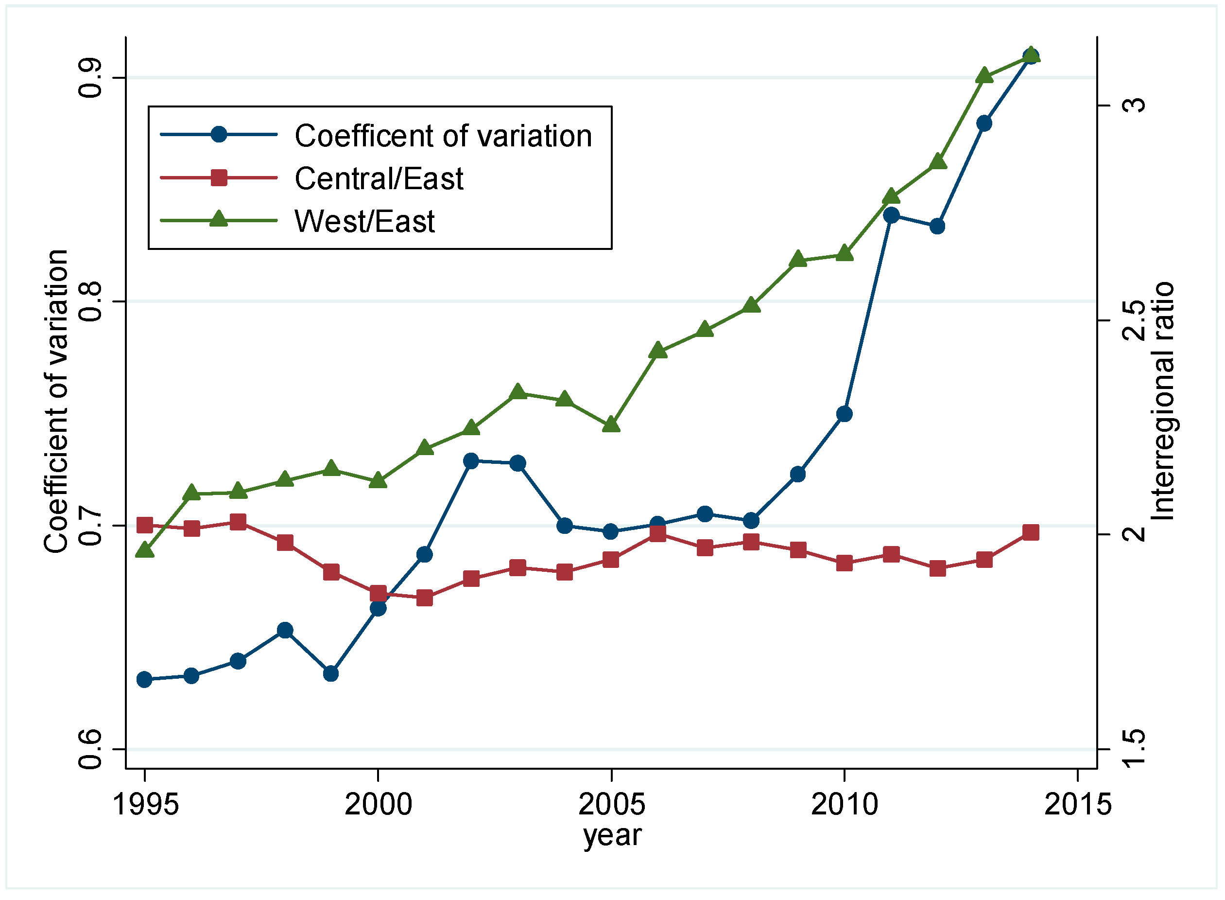
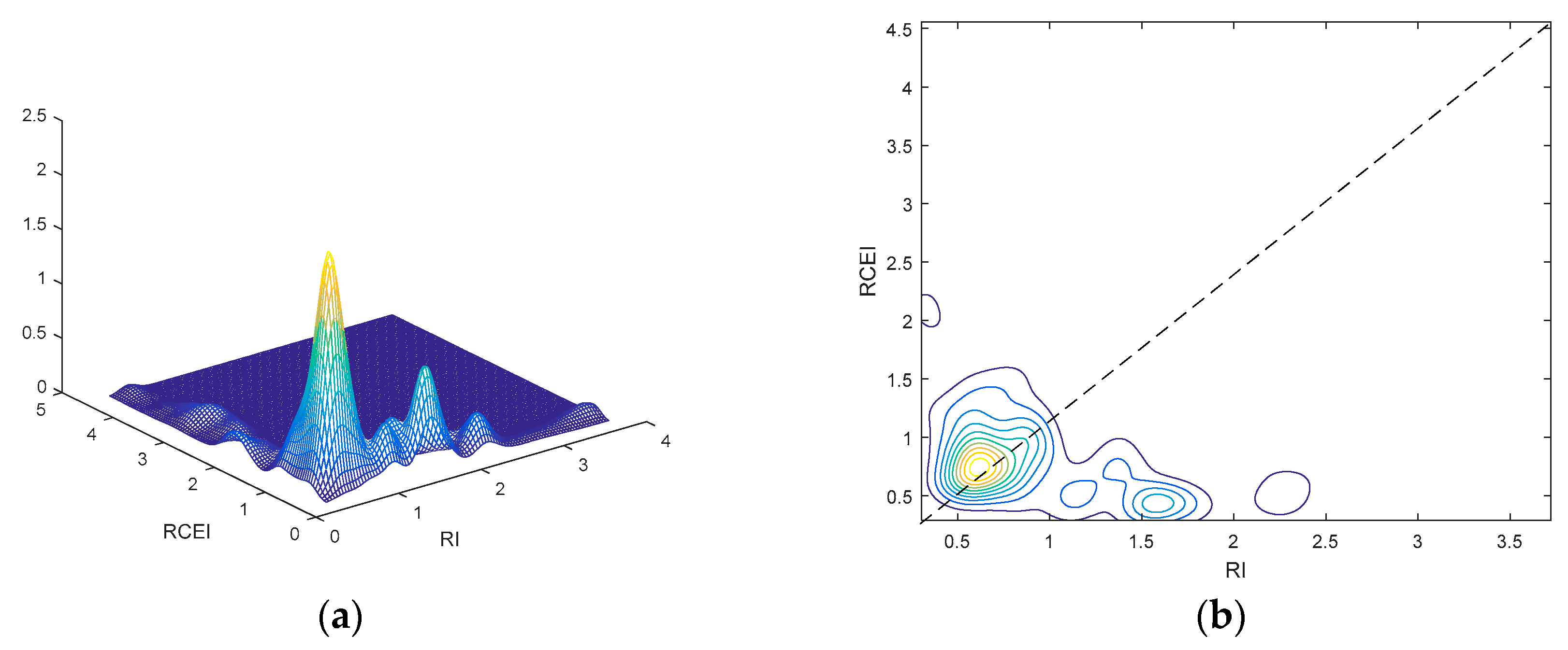
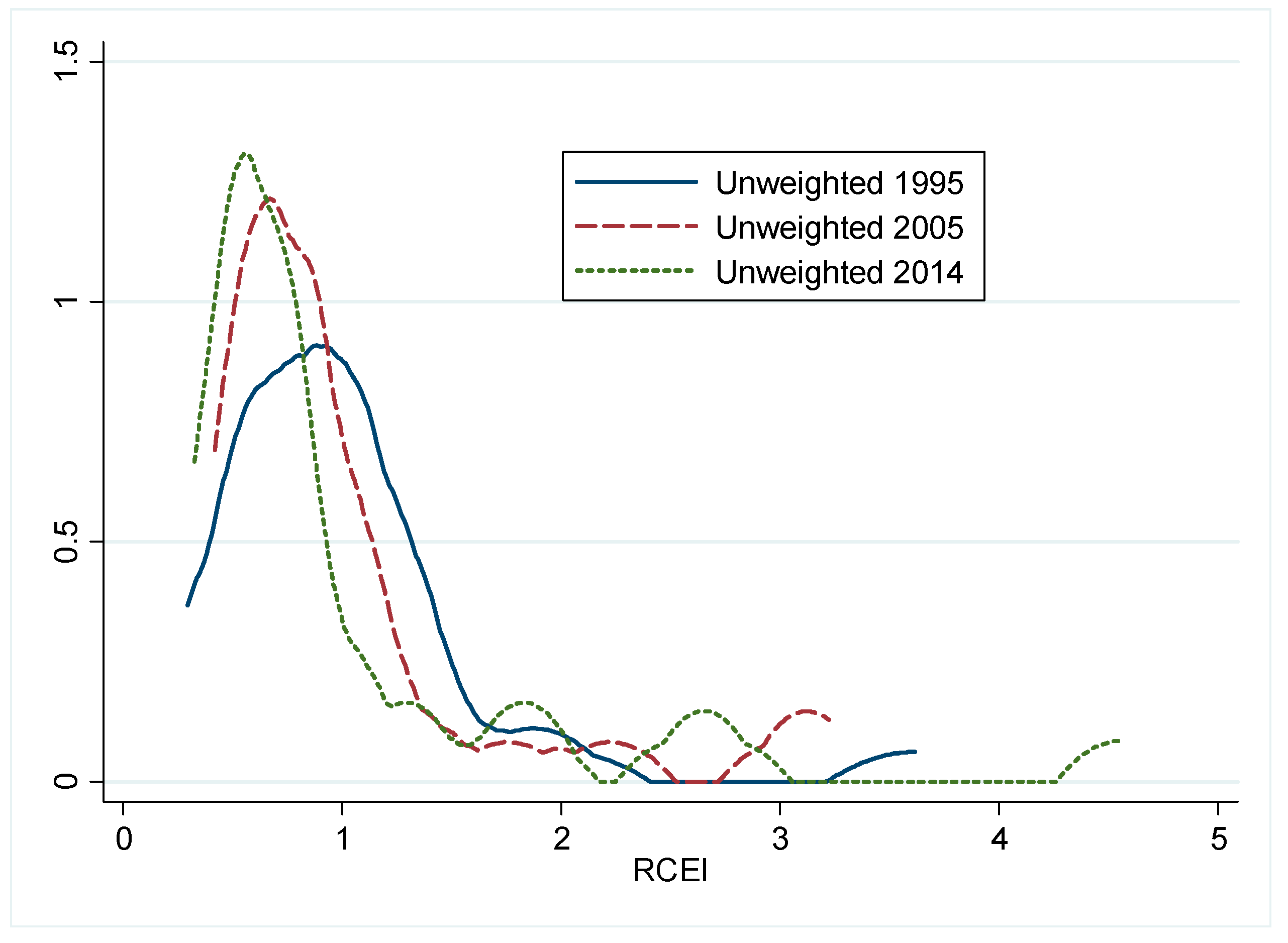
The result shows that Chinese provincial CO₂ emissions intensity has a dispersion trend in general. This dispersion is mainly driven by the increase of CO₂ emissions intensity in the western region relative to the eastern and central regions. The paper finds more persistence in provinces with low CO₂ emissions intensity and more mobility in provinces with high CO₂ emissions intensity. Convergence clubs can be observed in the long-run steady state. The intra-distribution dynamics shows that most provinces converge into the high CO₂ emissions intensity end. This indicates the deterioration in the evolution trend of CO₂ emissions intensity. 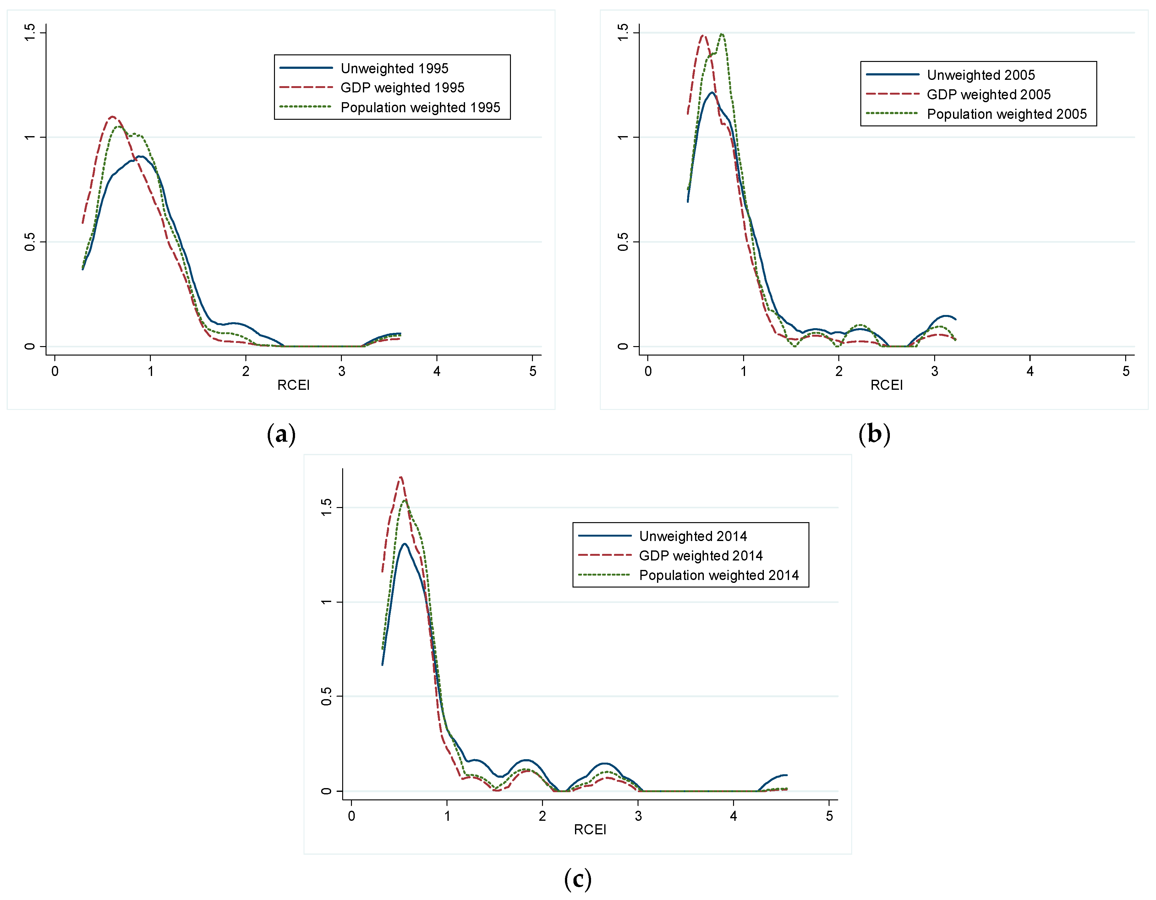In general, different from existing studies [1,2,3,4,5], our findings show that divergence, polarization, and stratification are the dominant characteristics in the distribution dynamics of CO₂ emissions intensity across Chinese provinces. Weighting by economy and population sizes has a significant impact on the distribution dynamics of CO₂ emissions intensity. It increases the peak in the high CO₂ emissions intensity end, but reduces the peak in the low CO₂ emissions intensity end. Neglecting economic and population sizes may underestimate the deterioration in the long-run steady state. The analysis of the two sub-periods shows that the deterioration is more significant in the sub-period 2005–2014 than in the sub-period 1995–2005. The conditional analysis indicates that conditioning on space and income cannot eliminate the multimodality in the ergodic distribution, implying that the convergence clubs in the long-run steady state are not determined by space and income in general. However, the result shows that capital intensity has a significant impact on the formation of convergence clubs in the high CO₂ emissions intensity end.

The results of this paper have important policy implications. First, the lack of convergence and the existence of convergence clubs in the distribution of CO₂ emissions intensity show that the market itself cannot automatically reduce environmental pollutants. Policies focused on technological spillover and industry upgrading are required to promote convergence in CO₂ emissions intensity. For example, Ninxia, which had the highest CO₂ emissions intensity in recent years, has a large share of heavy industries, such as coal mining, metallurgy, and mechanical industry. Therefore, technological progress and industry upgrading are the most efficient way to reduce CO₂ emissions intensity. Second, in China, CO₂ emissions reduction targets are assigned at the provincial level. However, provinces differ greatly in terms of their economy and population sizes. Hence, economy and population sizes should be considered in policy-making. Considering the deterioration in the intra-distribution of CO₂ emissions intensity, the central government should assign tougher targets to those provinces that have a tendency to increase their relative CO₂ emissions intensity, particularly those with a high CO₂ emissions intensity.

References

1. Huang, B.; Meng, L. Convergence of per capita carbon dioxide emissions in urban China: A spatio-temporal perspective. Appl. Geogr. 2013, 40, 21–29. [Google Scholar] [CrossRef]
2. Wang, J.; Zhang, K. Convergence of carbon dioxide emissions in different sectors in China. Energy 2014, 65, 605–611. [Google Scholar] [CrossRef]
3. Wang, Y.; Zhang, P.; Huang, D.; Cai, C. Convergence behavior of carbon dioxide emissions in China. Econ. Model. 2014, 43, 75–80. [Google Scholar] [CrossRef]
4. Hao, Y.; Liao, H.; Wei, Y.M. Is China’s carbon reduction target allocation reasonable? An analysis based on carbon intensity convergence. Appl. Energy 2015, 142, 229–239. [Google Scholar] [CrossRef]
5. Zhao, X.; Burnett, J.W.; Lacombe, D.J. Province-level convergence of China’s carbon dioxide emissions. Appl. Energy 2015, 150, 286–295. [Google Scholar] [CrossRef]
6. Barro, R.J.; Sala-i-Martin, X. Convergence. J. Political Econ. 1992, 100, 223–251. [Google Scholar] [CrossRef] [Green Version]
7. Stern, D.I. The Environmental Kuznets Curve: A Primer; Working Paper 2014; Centre for Climate Economics & Policy, Crawford School of Public Policy, The Australian National University: Canberra, Australia, 2014. [Google Scholar]
8. Kijima, M.; Nishide, K.; Ohyama, A. Economic models for the environmental Kuznets curve: A survey. J. Econ. Dyn. Control 2010, 34, 1187–1201. [Google Scholar] [CrossRef]
9. Pasten, R.; Figueroa, E. The environmental Kuznets curve: A survey of the theoretical literature. Int. Rev. Environ. Resour. Econ. 2012, 6, 195–224. [Google Scholar] [CrossRef]
10. Strazicich, M.C.; List, J.A. Are CO2 emission levels converging among industrial countries? Environ. Resour. Econ. 2003, 24, 263–271. [Google Scholar] [CrossRef]
11. Romero-Ávila, D. Convergence in carbon dioxide emissions among industrialised countries revisited. Energy Econ. 2008, 30, 2265–2282. [Google Scholar] [CrossRef]
12. Westerlund, J.; Basher, S.A. Testing for convergence in carbon dioxide emissions using a century of panel data. Environ. Resour. Econ. 2008, 40, 109–120. [Google Scholar] [CrossRef] [Green Version]
13. Barassi, M.R.; Cole, M.A.; Elliott, R.J.R. Stochastic divergence or convergence of per capita carbon dioxide emissions: Re-examining the evidence. Environ. Resour. Econ. 2008, 40, 121–137. [Google Scholar] [CrossRef]
14. Lee, C.C.; Chang, C.P. Stochastic convergence of per capita carbon dioxide emissions and multiple structural breaks in OECD countries. Econ. Model. 2009, 26, 1375–1381. [Google Scholar] [CrossRef]
15. Nourry, M. Re-examining the empirical evidence for stochastic convergence of two air pollutants with a pair-wise approach. Environ. Resour. Econ. 2009, 44, 555–570. [Google Scholar] [CrossRef]
16. Jobert, T.; Karanfil, F.; Tykhonenko, A. Convergence of per capita carbon dioxide emissions in the EU: Legend or reality? Energy Econ. 2010, 32, 1364–1373. [Google Scholar] [CrossRef]
17. Panopoulou, E.; Pantelidis, T. Club Convergence in Carbon Dioxide Emissions. Environ. Resour. Econ. 2009, 44, 47–70. [Google Scholar] [CrossRef]
18. Herrerias, M.J. The environmental convergence hypothesis: Carbon dioxide emissions according to the source of energy. Energy Policy 2013, 61, 1140–1150. [Google Scholar] [CrossRef]
19. El-Montasser, G.; Inglesi-Lotz, R.; Gupta, R. Convergence of greenhouse gas emissions among G7 countries. Appl. Econ. 2015, 47, 6543–6552. [Google Scholar] [CrossRef]
20. Van, P.N. Distribution dynamics of CO2 emissions. Environ. Resour. Econ. 2005, 32, 495–508. [Google Scholar]
21. Aldy, J.E. Per capita carbon dioxide emissions: Convergence or divergence? Environ. Resour. Econ. 2006, 33, 533–555. [Google Scholar] [CrossRef]
22. Ezcurra, R. Is there cross-country convergence in carbon dioxide emissions? Energy Policy 2007, 35, 1363–1372. [Google Scholar] [CrossRef]
23. Criado, C.O.; Grether, J.-M. Convergence in per capita CO2 emissions: A robust distributional approach. Environ. Resour. Econ. 2011, 33, 637–665. [Google Scholar] [CrossRef]
24. Herrerias, M.J. CO2 weighted convergence across the EU-25 countries (1920–2007). Appl. Energy 2012, 92, 9–16. [Google Scholar] [CrossRef]
25. Duro, J.A. International mobility in carbon dioxide emissions. Energy Policy 2013, 55, 208–216. [Google Scholar] [CrossRef]
26. Li, K.; Lin, B. Metafroniter energy efficiency with CO2 emissions and its convergence analysis for China. Energy Econ. 2015, 48, 230–241. [Google Scholar] [CrossRef]
27. Quah, D.T. Empirical cross-section dynamics in economic growth. Eur. Econ. Rev. 1993, 37, 426–434. [Google Scholar] [CrossRef]
28. Quah, D.T. Twin peaks: Growth and convergence in models of distribution dynamics. Econ. J. 1996, 106, 1045–1055. [Google Scholar] [CrossRef]
29. Quah, D.T. Empirics for growth and distribution: Stratification, polarization, and convergence clubs. J. Econ. Growth 1997, 2, 27–59. [Google Scholar] [CrossRef]
30. Silverman, B.W. Density Estimation for Statistics and Data Analysis; CRC Press: Boca Raton, FL, USA, 1986; pp. 40–42. [Google Scholar]
31. National Bureau of Statistics of China. China Compendium of Statistics 1949–2008; China Statistics Press: Beijing, China, 2010. (In Chinese) [Google Scholar]
32. National Bureau of Statistics of China. China Energy Statistical Yearbook; China Statistics Press: Beijing, China, 1996–2015. (In Chinese) [Google Scholar]
33. National Bureau of Statistics of China. China Statistical Yearbook; China Statistics Press: Beijing, China, 1996–2015. (In Chinese) [Google Scholar]
34. Intergovernmental Panel on Climate Change. IPCC Guidelines for National Greenhouse Gas Inventories; Institute for Global Environmental Strategies: Kanagawa, Japan, 2006. [Google Scholar]
35. Wu, Y. China’s Capital Stock Series by Region and Sector; Discussion Paper 09.02; The University of Western Australia: Crawley, Australia, 2009. [Google Scholar]
36. Bassetti, T.; Benos, N.; Karagiannis, S. CO2 emissions and income dynamics: What does the global evidence tell us? Environ. Resour. Econ. 2013, 54, 101–125. [Google Scholar] [CrossRef]
Figure 1. The coefficient of variation and ratio of the western region and central region to the eastern region in terms of CO2 emissions intensity.
Sustainability 09 00101 g001
Figure 2. The kernel density distributions of RCEI in representative years.
Sustainability 09 00101 g002
Figure 3. The weighted distributions of RCEI in 1995 (a); 2005 (b); and 2014 (c).
Sustainability 09 00101 g003
Figure 4. The distribution dynamics of unweighted and weighted RCEI with annual transition, 1995–2014. Note: The solid, dashed, and dotted lines show the unweighted, GDP-weighted, and population-weighted RCEI, respectively. (a) Three-dimensional plot (unweighted); (b) Contour map (unweighted); (c) Net transition probability plot (unweighted); (d) Ergodic distribution (unweighted); (e) Net transition probability plot (weighted); (f) Ergodic distribution (weighted).
Sustainability 09 00101 g004
Figure 5. Net transition probability and ergodic distribution for weighted and unweighted RCEI with annual transition, 1995–2005. Note: The solid, dashed, and dotted lines show the unweighted, GDP-weighted, and population-weighted RCEI, respectively. (a) Three-dimensional plot (unweighted); (b) Contour map (unweighted); (c) Net transition probability plot; (d) Ergodic distribution.
Sustainability 09 00101 g005
Figure 6. Net transition probability and ergodic distribution for weighted and unweighted RCEI with annual transition, 2005–2014. Note: The solid, dashed, and dotted lines show the unweighted, GDP-weighted, and population-weighted RCEI, respectively. (a) Three-dimensional plot (unweighted); (b) Contour map (unweighted); (c) Net transition probability plot; (d) Ergodic distribution.
Sustainability 09 00101 g006
Figure 7. The distribution dynamics of the space conditional RPCG with annual transition, 1978–2013. Note: The solid and dashed lines show the conditional and unconditional distributions, respectively. (a) Three-dimensional plot of joint distribution; (b) Contour plot of joint distribution; (c) Three-dimensional plot; (d) Contour plot; (e) Net transition probability plot; (f) Ergodic distribution.
Sustainability 09 00101 g007
Figure 8. The distribution dynamics of the income-conditional RCEI with annual transition, 1995–2014. Note: The solid and dashed lines show the conditional and unconditional distributions, respectively. (a) Three-dimensional plot of joint distribution; (b) Contour plot of joint distribution; (c) Three-dimensional plot; (d) Contour plot; (e) Net transition probability plot; (f) Ergodic distribution.
Sustainability 09 00101 g008aSustainability 09 00101 g008b
Figure 9. The distribution dynamics of the capital conditional RCEI with annual transition, 1995–2014. Note: The solid and dashed lines show the conditional and unconditional distributions, respectively. (a) Three-dimensional plot of joint distribution; (b) Contour plot of joint distribution; (c) Three-dimensional plot; (d) Contour plot; (e) Net transition probability plot; (f) Ergodic distribution.
Sustainability 09 00101 g009