
Mapping Social Vulnerability to Air Pollution: A Case Study of the Yangtze River Delta Region, China

Abstract
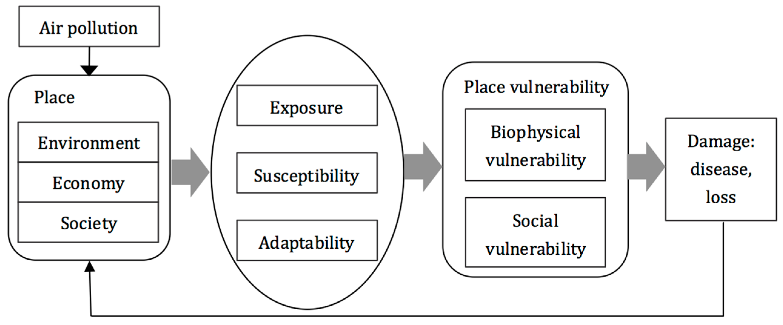
:1. Introduction
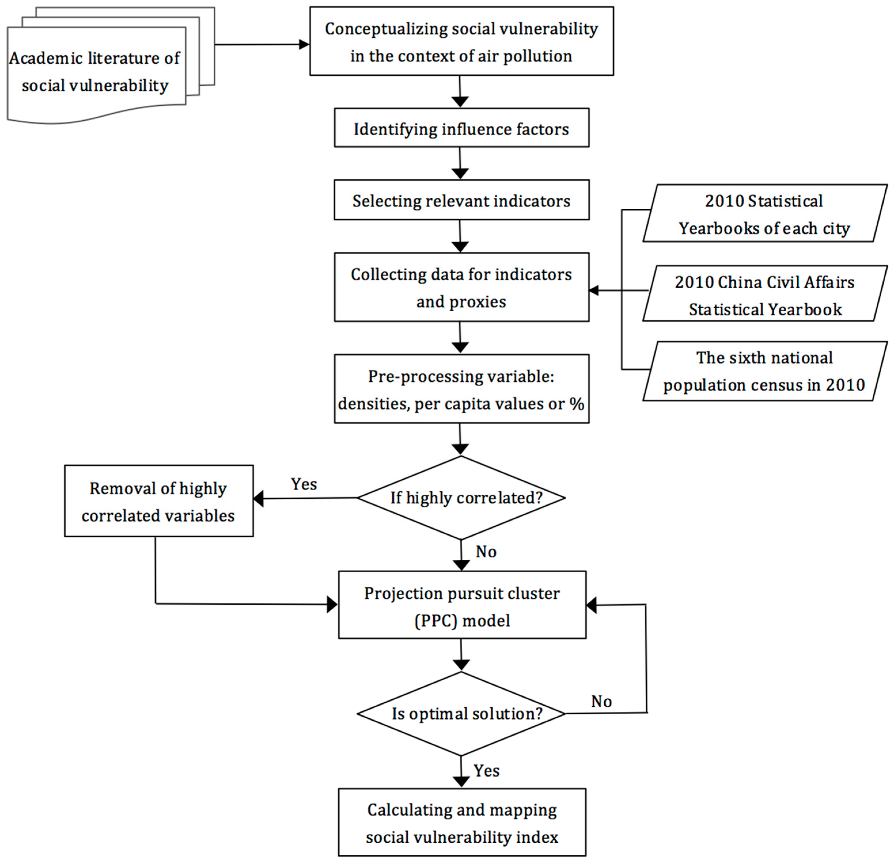
2. Materials and Methods
2.1. Data
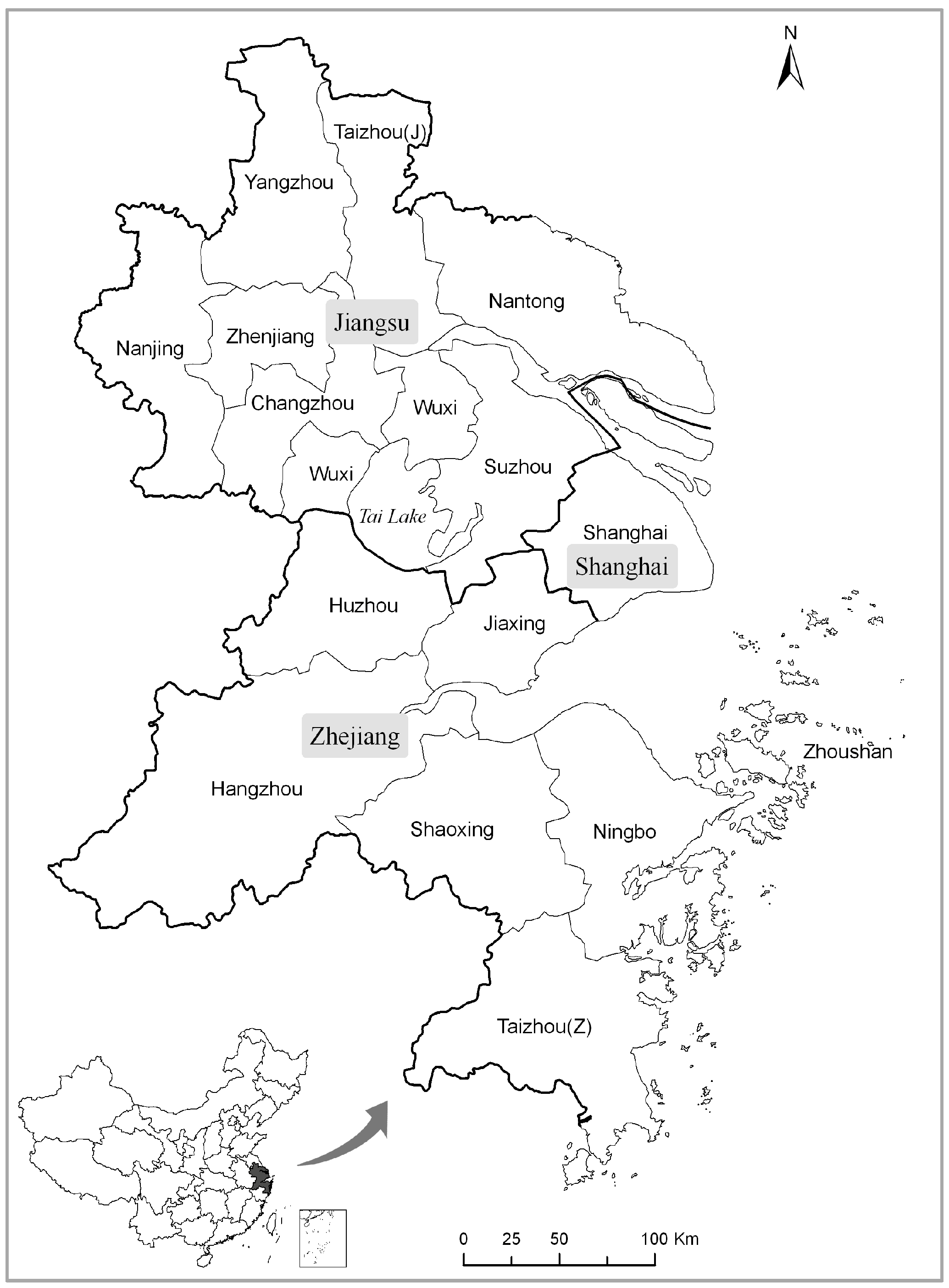
2.2. Case Study: the Yangtze River Delta Region
2.3. Research Method: the Projection Pursuit Cluster (PPC) Model
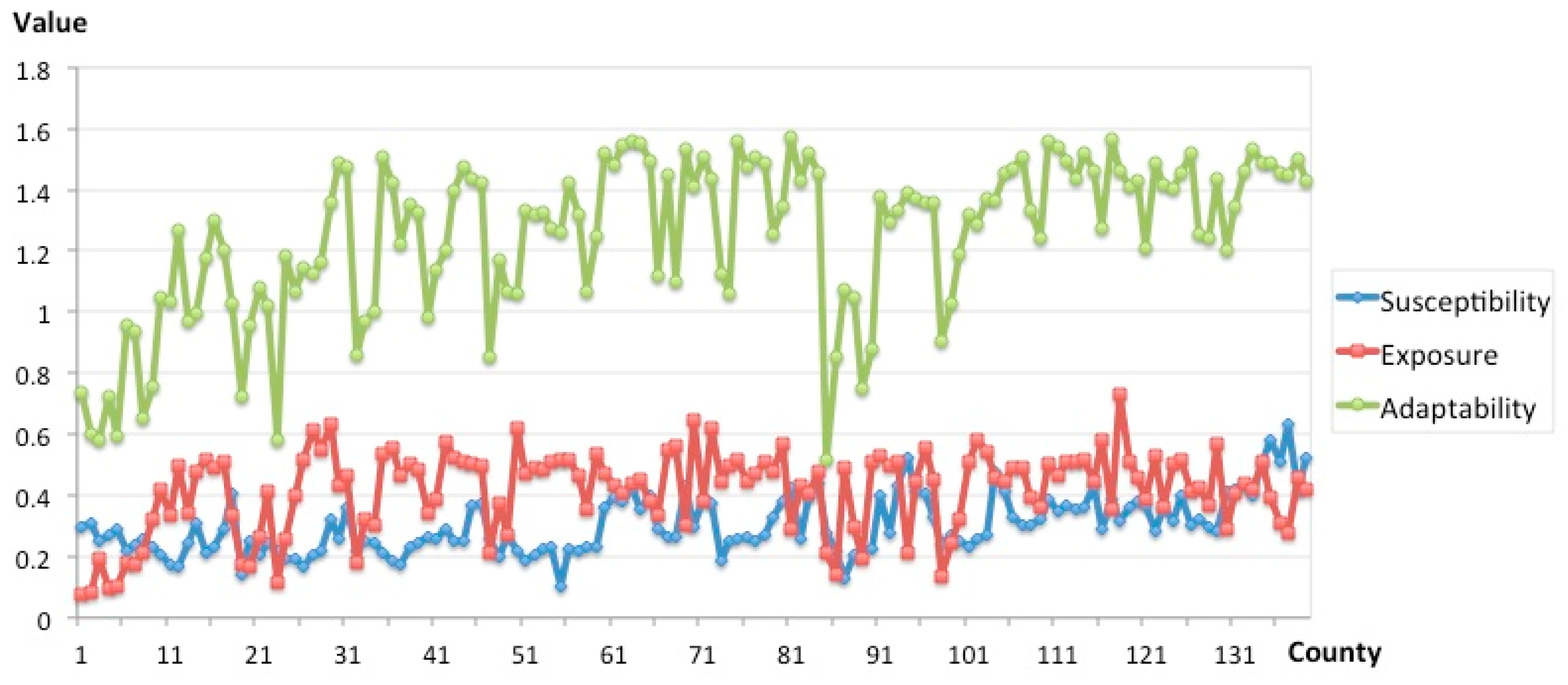
3. Results and Discussion
4. Conclusions
Acknowledgments
Author Contributions
Conflicts of Interest
References
- Lo, K. A critical review of China’s rapidly developing renewable energy and energy efficiency policies. Renew. Sustain. Energy Rev. 2014, 29, 508–516. [Google Scholar] [CrossRef]
- Yang, K.; Yang, Y.; Zhu, Y.; Li, C.; Meng, C. Social and economic drivers of PM2.5 and their spatial relationship in China. Geogr. Res. 2016, 35, 1051–1060. [Google Scholar] [CrossRef]
- Zheng, S.; Yi, H.; Li, H. The impacts of provincial energy and environmental policies on air pollution control in China. Renew. Sustain. Energy Rev. 2015, 49, 386–394. [Google Scholar] [CrossRef]
- Zou, B.; Pu, Q.; Luo, Y.; Tian, Y.; Zhang, W. On the complex indicative system based on the spatially divided urban areas for PM2.5 pollution&control. J. Saf. Environ. 2016, 16, 337–342. [Google Scholar]
- Kan, H. Environment and health in China: Challenges and opportunities. Environ. Health Perspect. 2009, 117, A530–A531. [Google Scholar] [CrossRef] [PubMed]
- Lin, H.; Liu, T.; Xiao, J.; Zeng, W.; Li, X.; Guo, L.; Xu, Y.; Zhang, Y.; Vaughn, M.G.; Nelson, E.J.; et al. Quantifying short-term and long-term health benefits of attaining ambient fine particulate pollution standards in Guangzhou, China. Atmos. Environ. 2016, 137, 38–44. [Google Scholar] [CrossRef]
- Fujii, H.; Managi, S.; Kaneko, S. Decomposition analysis of air pollution abatement in China: Empirical study for ten industrial sectors from 1998 to 2009. J. Clean. Prod. 2013, 59, 22–31. [Google Scholar] [CrossRef]
- Wang, P.; Wang, G. PM2.5 Pollution in China and its harmfulness to human health. Sci. Technol. Rev. 2014, 32, 72–78. [Google Scholar]
- Chen, X.; Shao, S.; Tian, Z.; Xie, Z.; Yin, P. Impacts of air pollution and its spatial spillover effect on public health based on China’s big data sample. J. Clean. Prod. 2017, 142, 915–925. [Google Scholar] [CrossRef]
- Li, L.; Lin, G.Z.; Liu, H.Z.; Guo, Y.; Ou, C.Q.; Chen, P.Y. Can the Air Pollution Index be used to communicate the health risks of air pollution? Environ. Pollut. 2015, 205, 153–160. [Google Scholar] [CrossRef] [PubMed]
- Feretis, E.; Theodorakopoulos, P.; Varotsos, C.; Efstathiou, M.; Tzanis, C.; Xirou, T.; Alexandridou, N.; Aggelou, M. On the plausible association between environmental conditions and human eye damage. Environ. Sci. Pollut. Res. 2002, 9, 163–165. [Google Scholar] [CrossRef]
- Ferm, M.; Watt, J.; O’Hanlon, S.; De Santis, F.; Varotsos, C. Deposition measurement of particulate matter in connection with corrosion studies. Anal. Bioanal. Chem. 2006, 384, 1320–1330. [Google Scholar] [CrossRef] [PubMed]
- Ferm, M.; de Santis, F.; Varotsos, C. Nitric acid measurements in connection with corrosion studies. Atmos. Environ. 2005, 39, 6664–6672. [Google Scholar] [CrossRef]
- Ziemke, J.R.; Chandra, S.; Herman, J.; Varotsos, C. Erythemally weighted UV trends over northern latitudes derived from Nimbus 7 TOMS measurements. J. Geophys. Res. 2000, 105, 7373. [Google Scholar] [CrossRef]
- Katsambas, A.; Varotsos, C.A.; Veziryianni, G.; Antoniou, C. Surface solar ultraviolet radiation: A theoretical approach of the SUVR reaching the ground in Athens, Greece. Environ. Sci. Pollut. Res. Int. 1997, 4, 69–73. [Google Scholar] [CrossRef] [PubMed]
- Hizbaron, D.R.; Baiquni, M.; Sartohadi, J.; Rijanta, R. Urban vulnerability in Bantul District, Indonesia—Towards safer and sustainable development. Sustainability 2012, 4, 2022–2037. [Google Scholar] [CrossRef]
- Zhang, Y.; Shen, J.; Ding, F.; Li, Y.; He, L. Vulnerability assessment of atmospheric environment driven by human impacts. Sci. Total Environ. 2016, 571, 778–790. [Google Scholar] [CrossRef] [PubMed]
- Pincetl, S.; Chester, M.; Eisenman, D. Urban heat stress vulnerability in the U.S. Southwest : The role of sociotechnical systems. Sustainability 2016, 8, 842. [Google Scholar] [CrossRef]
- Nguyen, L.D.; Raabe, K.; Grote, U. Rural-Urban migration, household vulnerability, and welfare in Vietnam. World Dev. 2015, 71, 79–93. [Google Scholar] [CrossRef]
- Wisner, B.; Blaikie, P.; Cannon, T.; Davis, I. At Risk: Natural Hazards, People’s Vulnerability, and Disasters, 2nd ed.; Routledge: London, UK, 2004. [Google Scholar]
- Willis, I. A brief Note Defining Vulnerability and Risk. Available online: https://iainwillis.wordpress.com/2012/01/18/a-brief-note-defining-vulnerability-and-risk/ (accessed on 20 June 2011).
- Fussel, H.-M. Vulnerability : A generally applicable conceptual framework for climate change research. Glob. Environ. Chang. 2007, 17, 155–167. [Google Scholar] [CrossRef]
- Li, X.; Zhou, Y.; Tian, B.; Kuang, R.; Wang, L. GIS-based methodology for erosion risk assessment of the muddy coast in the Yangtze Delta. Ocean Coast. Manag. 2015, 108, 97–108. [Google Scholar] [CrossRef]
- Janssen, M.A.; Schoon, M.L.; Ke, W.; Bo, K. Scholarly networks on resilience, vulnerability and adaptation within the human dimensions of global environmental change. Glob. Environ. Chang. 2006, 16, 240–252. [Google Scholar] [CrossRef]
- Zhou, Y.; Li, N.; Wu, W.; Wu, J.; Shi, P. Local spatial and temporal factors influencing population and societal vulnerability to natural disasters. Risk Anal. 2014, 34, 614–639. [Google Scholar] [CrossRef] [PubMed]
- Dow, K. Exploring differences in our common future(s): The meaning of vulnerability to global environmental change. Geoforum 1992, 23, 417–436. [Google Scholar] [CrossRef]
- Cutter, S.L. Vulnerability to environmental hazards. Prog. Hum. Geogr. 1996, 20, 529–539. [Google Scholar] [CrossRef]
- Birkmann, J. Measuring vulnerability to promote disaster-resilient societies : Conceptual frameworks and definitions. In Measuring Vulnerability to Natural Harzards: Towards Disaster Resilient Societies; United Nations University Press: New York, NY, USA, 2006; pp. 9–54. [Google Scholar]
- Cutter, S.L.; Carolina, S.; Boruff, B.J.; Shirley, W.L.; Carolina, S.; Shirley, W.L.; Carolina, S. Social vulnerability to environmental hazards. Soc. Sci. Q. 2003, 84, 242–261. [Google Scholar] [CrossRef]
- Ge, Y.; Liu, J.; Li, F.; Shi, P. Quantifying social vulnerability for flood disasters of insurance company. J. Southeast Univ. 2008, 24, 147–150. [Google Scholar]
- Neil, L.; Conde, C.; Kulkarni, J.; Nyong, A.; Pulbin, J. Climate Change and Vulnerability; Earthscan: London, UK; Sterling, VA, USA, 2008. [Google Scholar]
- Blaikie, P.; Cannon, T.; Davis, I.; Wisner, B. At Risk: Natural Hazards, People’s Vulnerability, and Disasters; Routledge: London, UK, 1994. [Google Scholar]
- Turner, B.L., II; Kasperson, R.E.; Matson, P.A.; Mccarthy, J.J.; Corell, R.W.; Christensen, L.; Eckley, N.; Kasperson, J.X.; Luers, A.; Martello, M.L.; et al. A framework for vulnerability analysis in sustainability science. PNAS 2003, 100, 14. [Google Scholar] [CrossRef] [PubMed]
- Chen, W.; Cutter, S.L.; Emrich, C.T.; Shi, P. Measuring social vulnerability to natural hazards in the Yangtze River Delta region, China. Int. J. Disaster Risk Sci. 2013, 4, 169–181. [Google Scholar] [CrossRef]
- Dwyer, A.; Zoppou, C.; Nielsen, O.; Day, S.; Roberts, S. Quantifying Social Vulnerability: A Methodology for Identifying Those at Risk to Natural Hazards; Geoscience Australia: Canberra, Australia, 2004.
- Ge, Y.; Dou, W.; Gu, Z.; Qian, X. Assessment of social vulnerability to natural hazards in the Yangtze River Delta, China. Stoch. Environ. Res. Risk Assess. 2013, 27, 1899–1908. [Google Scholar] [CrossRef]
- New Indicators of Vulnerability and Adaptive Capacity. Available online: http://www.tyndall.ac.uk/content/new-indicators-vulnerability-and-adaptive-capacity (accessed on 11 January 2017).
- Wood, N.J.; Burton, C.G.; Cutter, S.L. Community variations in social vulnerability to Cascadia-related tsunamis in the U.S. Pacific Northwest. Nat. Hazards 2010, 52, 369–389. [Google Scholar] [CrossRef]
- Holand, I.S.; Lujala, P. Replicating and adapting an index of social vulnerability to a new context: A comparison study for Norway. Prof. Geogr. 2013, 65, 312–328. [Google Scholar] [CrossRef]
- Zhou, Y.; Li, N.; Wu, W.; Wu, J. Assessment of provincial social vulnerability to natural disasters in China. Nat. Hazards 2014, 71, 2165–2186. [Google Scholar] [CrossRef]
- Cutter, S.L.; Finch, C. Temporal and spatial changes in social vulnerability to natural hazards. Proc. Natl. Acad. Sci. USA 2008, 7, 2301–2306. [Google Scholar] [CrossRef] [PubMed]
- Tierney, K. Social inequality, hazards, and disasters. In On Risk and Disaster: Lessons from Hurricane Katrina; Daniels, R.J., Kettl, E.F., Kunreuther, H., Eds.; University of Pennsylvania Press: Philadephia, PA, USA, 2006; pp. 109–128. [Google Scholar]
- Wei, Y.M.; Fan, Y.; Lu, C.; Tsai, H.T. The assessment of vulnerability to natural disasters in China by using the DEA method. Environ. Impact Assess. Rev. 2004, 24, 427–439. [Google Scholar] [CrossRef]
- Huang, J.; Liu, Y.; Ma, L. Assessment of regional vulnerability to natural hazards in China using a DEA model. Int. J. Disaster Risk Sci. 2011, 2, 41–48. [Google Scholar] [CrossRef]
- Fan, Y.; Luo, Y.; Chen, Q. Establishment of weight about vulnerability indexes of a hazard bearing body. J. Catastr. 2001, 16, 85–87. [Google Scholar]
- Roy, D.C.; Blaschke, T. Spatial vulnerability assessment of floods in the coastal regions of Bangladesh. Geomat. Nat. Hazards Risk 2013, 5705, 1–24. [Google Scholar] [CrossRef]
- Rygel, L.; O’Sullivan, D.; Yarnal, B. A method for constructing a social vulnerability index: An application to hurricane storm surges in a developed country. Mitig. Adapt. Strateg. Glob. Chang. 2006, 11, 741–764. [Google Scholar] [CrossRef]
- Frigerio, I.; de Amicis, M. Mapping social vulnerability to natural hazards in Italy : A suitable tool for risk mitigation strategies. Environ. Sci. Policy 2016, 63, 187–196. [Google Scholar] [CrossRef]
- Frigerio, I.; Ventura, S.; Strigaro, D.; Mattavelli, M.; de Amicis, M.; Mugnano, S.; Bof, M. A GIS-based approach to identify the spatial variability of social vulnerability to seismic hazard in Italy. Appl. Geogr. 2016, 74, 12–22. [Google Scholar] [CrossRef]
- Carpiano, R.M.; Link, B.G.; Phelan, J.C. Social Inequality and Health: Future direction for the fundamental cause explanation. In Social Class: How Does It Works? Russell Sage Foundation: New York, NY, USA, 2008; pp. 232–263. [Google Scholar]
- Makri, A.; Stilianakis, N.I. Vulnerability to air pollution health effects. Int. J. Hyg. Environ. Health 2008, 211, 326–336. [Google Scholar] [CrossRef] [PubMed]
- Jain, S.; Khare, M. Urban air quality in mega cities : A case study of Delhi City using vulnerability analysis. Environ. Monit Assess 2008, 136, 257–265. [Google Scholar] [CrossRef] [PubMed]
- Flanagan, B.E.; Gregory, E.W.; Hallisey, E.J.; Heitgerd, J.L.; Lewis, B. A social vulnerability index for disaster management. J. Homel. Secur. Emerg. Manag. 2011, 8, 1–22. [Google Scholar] [CrossRef]
- Bentayeb, M.; Simoni, M.; Baiz, N.; Norback, D.; Baldacci, S.; Maio, S.; Viegi, G.; Annesi-Maesano, I. Adverse respiratory effects of outdoor air pollution in the elderly. Int. J. Tuberc. Lung Dis. 2012, 16, 1149–1161. [Google Scholar] [CrossRef] [PubMed]
- Simoni, M.; Baldacci, S.; Maio, S.; Cerrai, S.; Sarno, G.; Viegi, G. Adverse effects of outdoor pollution in the elderly. J. Thorac. Dis. 2015, 7, 34–45. [Google Scholar]
- World Health Organization (WHO). Effects of Air Pollution on Children’s Health and Development a Review of the Evidence Special Programme on Health and Environment; WHO: Copenhagen, Denmark, 2005. [Google Scholar]
- Morrow, B.H. Identifying and mapping community vulnerability. Disasters 1999, 23, 1–18. [Google Scholar] [CrossRef] [PubMed]
- Holand, I.S.; Lujala, P.; Rød, J.K. Social vulnerability assessment for Norway: A quantitative approach. Nor. Geogr. Tidsskr.-Nor. J. Geogr. 2011, 65, 1–17. [Google Scholar] [CrossRef]
- Wang, Q. Vulnerability analysis of cities to PM2.5. Mod. Bus. Trade Ind. 2014, 59–61. [Google Scholar]
- Finkelstein, M.M.; Jerrett, M.; Sears, M.R. Environmental inequality and circulatory disease mortality gradients. J. Epidemiol. Community Health 2005, 59, 481–487. [Google Scholar] [CrossRef] [PubMed]
- Finkelstein, M.M.; Jerrett, M.; DeLuca, P.; Finkelstein, N.; Verma, D.K.; Chapman, K.; Sears, M.R. Relation between income, air pollution and mortality: A cohort study. Can. Med. Assoc. J. 2003, 169, 397–402. [Google Scholar]
- Jerrett, M.; Burnett, R.T.; Brook, J.; Kanaroglou, P.; Giovis, C.; Finkelstein, N.; Hutchison, B. Do socioeconomic characteristics modify the short term association between air pollution and mortality? Evidence from a zonal time series in Hamilton, Canada. J. Epidemiol. Community Health 2004, 58, 31–40. [Google Scholar] [CrossRef] [PubMed]
- Wheeler, B.W.; Ben-Shlomo, Y. Environmental equity, air quality, socioeconomic status, and respiratory health: A linkage analysis of routine data from the health survey for England. J. Epidemiol. Community Health 2005, 59, 948–954. [Google Scholar] [CrossRef] [PubMed]
- Gunier, R.B.; Hertz, A.; von Behren, J.; Reynolds, P. Traffic density in California: Socioeconomic and ethnic differences among potentially exposed children. J. Expo. Anal. Environ. Epidemiol. 2003, 13, 240–246. [Google Scholar] [CrossRef] [PubMed]
- Mildrexler, D.; Yang, Z.; Cohen, W.B.; Bell, D.M. A forest vulnerability index based on drought and high temperatures. Remote Sens. Environ. 2015, 173, 314–325. [Google Scholar] [CrossRef]
- Filleul, L.; Rondeau, V.; Cantagrel, A.; Dartigues, J.-F.; Tessier, J.-F. Do subject characteristics modify the effects of particulate air pollution on daily mortality among the elderly? J. Occup. Environ. Med. 2004, 46, 1115–1122. [Google Scholar] [CrossRef] [PubMed]
- Wang, T.; Jiang, F.; Deng, J.; Shen, Y.; Fu, Q.; Wang, Q.; Fu, Y.; Xu, J.; Zhang, D. Urban air quality and regional haze weather forecast for Yangtze River Delta region. Atmos. Environ. 2012, 58, 70–83. [Google Scholar] [CrossRef]
- Li, L.; Chen, C.H.; Fu, J.S.; Huang, C.; Streets, D.G.; Huang, H.Y.; Zhang, G.F.; Wang, Y.J.; Jang, C.J.; Wang, H.L.; et al. Air quality and emissions in the Yangtze River Delta, China. Atmos. Chem. Phys. 2011, 11, 1621–1639. [Google Scholar] [CrossRef] [Green Version]
- Sarkar, A.; Vulimiri, A.; Bose, S.; Paul, S.; Ray, S.S. Unsupervised hyperspectral image analysis with projection pursuit and MRF segmentation approach. In Proceedings of the International Conference on Artificial Intelligence and Pattern Recognition 2008, AIPR 2008, Orlando, FL, USA, 7–10 July 2008.
- Nason, G.P. Robust projection indices. J. R. Stat. Soc. Ser. B 2001, 63, 551–567. [Google Scholar] [CrossRef]


| Factors | Indicator Names | Description |
|---|---|---|
| Age | Children and Elderly | Children and the elderly are especially sensitive to air pollution. Physiologic immaturity and developmental changes account for children’s susceptibility to air pollutants. For older people, comorbidity, physical fragility and less appropriate immune responses decrease their coping capacity. Source: [10,29,53,54,55,56]. |
| Gender | Female | Women can have a more difficult time during recovery than men, often due to lower wages, and family care responsibilities. Source: [27,29,32] |
| Ethnicity | Ethnicity | Imposes language and cultural barriers that affect the ability to seek, find or understand warning information and access recovery information. Source: [29] |
| Education | Illiterate and Educated | People highly educated are more likely to have better employment prospects, which results in better economic conditions and more resources to take precaution against air pollution. Source: [29,57,58,59] |
| Individual economic status | Unemployed;Poor | Low-income individuals often exposure to hazardous pollution environment or can’t take enough actions to protect themselves against air pollution. Source: [2,60,61,62,63,64,65] |
| Population exposure | Urban resident; Employees in 2nd industry, mining, manufactory and construction; GDP in secondary sector; Population density | Urban residents expose to severer air pollution for ambient heavy traffic. High-exposure occupations lead to high health risk for potential cumulative effects in air pollution. The boom and bust economy of secondary sector may create more high-exposure occupation opportunities. Population density illustrates discrepancy of average exposure among regions. Source: [2,17,51,59,66]. |
| Regional resource | GDP; Green space coverage | “GDP” and “Green space coverage” demonstrate potential resources available for absorbing, reducing the adverse impact and recovering from losses more quickly. Source: [17,25,29,57] |
| Medical and management services | Beds and Physicians in hospital; Employees in management sector | Public medical services can help for recovery and mitigation. Employees in the sectors of management can reflect the capacity of environmental governance. Source: [25,29,59]. |
| No. | Indicator | Name | Description | Dimension of SVI | Impact to SVI |
|---|---|---|---|---|---|
| 1 | Children | CHILD | Percentage of population under 14 years old | Susceptibility | + |
| 2 | Elderly | ELD | Percentage of population over 65 years old | Susceptibility | + |
| 3 | Female | FEMALE | Percentage of female | Susceptibility | + |
| 4 | Ethnicity | ETHNICITY | Percentage of Ethnicity | Susceptibility | + |
| 5 | Illiterate | ILLITERATE | Percentage of illiterates among those aged 15 and over | Susceptibility | + |
| 6 | Poor | POOR | Percentage of recipients of subsistence allowances | Susceptibility | + |
| 7 | Unemployed | UNEMPLOY | Percentage of unemployed | Susceptibility | + |
| 8 | Population density | POPDENSITY | Population density | Exposure | + |
| 9 | Urban resident | URBAN | Percentage of urban residents | Exposure | + |
| 10 | Employees in 2nd industry | SECWORKER | Percentage of employed in secondary industry | Exposure | + |
| 11 | Employees in mining | MINING | Percentage of employed in mining | Exposure | + |
| 12 | Employees in manufactory | MANUFACT | Percentage of employed in manufactory | Exposure | + |
| 13 | Employees in construction | CONSTRUCT | Percentage of employed in construction | Exposure | + |
| 14 | GDP in secondary sector | INDUSTRY | Percentage of GDP in secondary sector | Exposure | + |
| 15 | GDP | P_GDP | Gross domestic product per capita | Adaptability | − |
| 16 | Educated | EDUCATE | Percentage higher education graduates | Adaptability | − |
| 17 | Beds in hospital | HOSBED | Number of beds in hospital per 1000 people | Adaptability | − |
| 18 | Physicians in hospital | HOSPHY | Number of physicians in hospital per 1000 people | Adaptability | − |
| 19 | Employees in management sector | ENWORKER | Percentage employees in the sectors of water conservancy, environment and public management | Adaptability | − |
| 20 | Green space coverage | GREEN | Ratio of open green space coverage | Adaptability | − |
| No. | Indicators | Weighting Values | No. | Indicators | Weighting Values |
|---|---|---|---|---|---|
| 1 | Children | 0.297 | 11 | Employees in mining | 0.274 |
| 2 | Elderly | 0.120 | 12 | Employees in construction | 0.166 |
| 3 | Female | 0.142 | 13 | GDP in secondary sector | 0.255 |
| 4 | Ethnicity | 0.082 | 14 | GDP | 0.188 |
| 5 | Illiterate | 0.245 | 15 | Educated | 0.416 |
| 6 | Poor | 0.063 | 16 | Beds in hospital | 0.283 |
| 7 | Unemployed | 0.040 | 17 | Physicians in hospital | 0.365 |
| 8 | Population density | 0.060 | 18 | Employees in management sector | 0.355 |
| 9 | Urban resident | 0.024 | 19 | Green space coverage | 0.044 |
| 10 | Employees in 2nd industry | 0.288 |
| SVI | YRD Region | Shanghai Municipality | Jiangsu Province | Zhejiang Province |
|---|---|---|---|---|
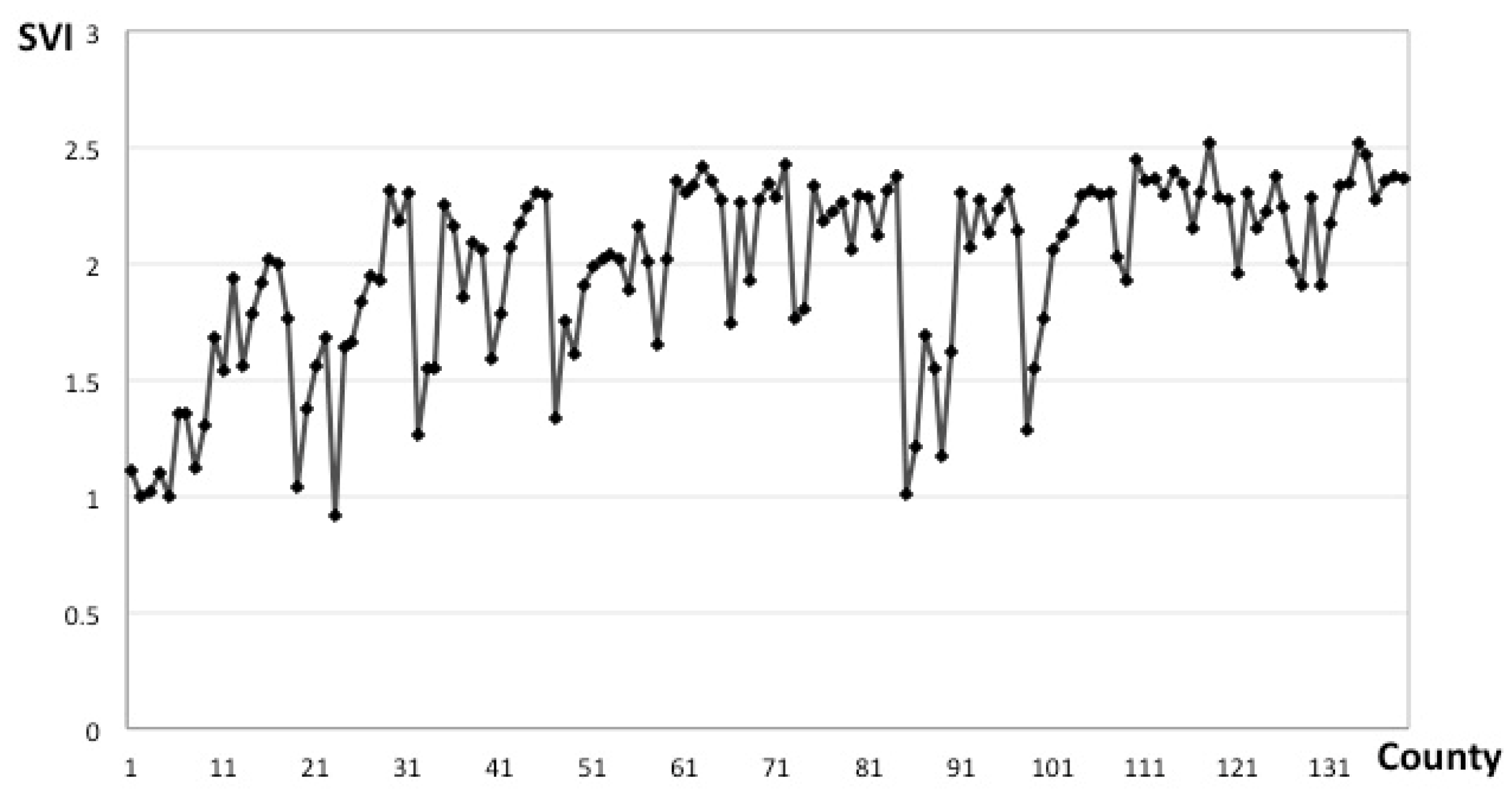
| Average | 1.970 | 1.474 | 1.989 | 2.110 |
| Minimum | 0.916 | 0.992 | 0.916 | 1.002 |
| Maximum | 2.516 | 2.021 | 2.429 | 2.516 |
| Level | SVI | SVI Dimension 1 | SVI Dimension 2 | SVI Dimension 3 | ||||
|---|---|---|---|---|---|---|---|---|
| Susceptibility | Exposure | Adaptability | ||||||
| Count | Percentage | Count | Percentage | Count | Percentage | Count | Percentage | |
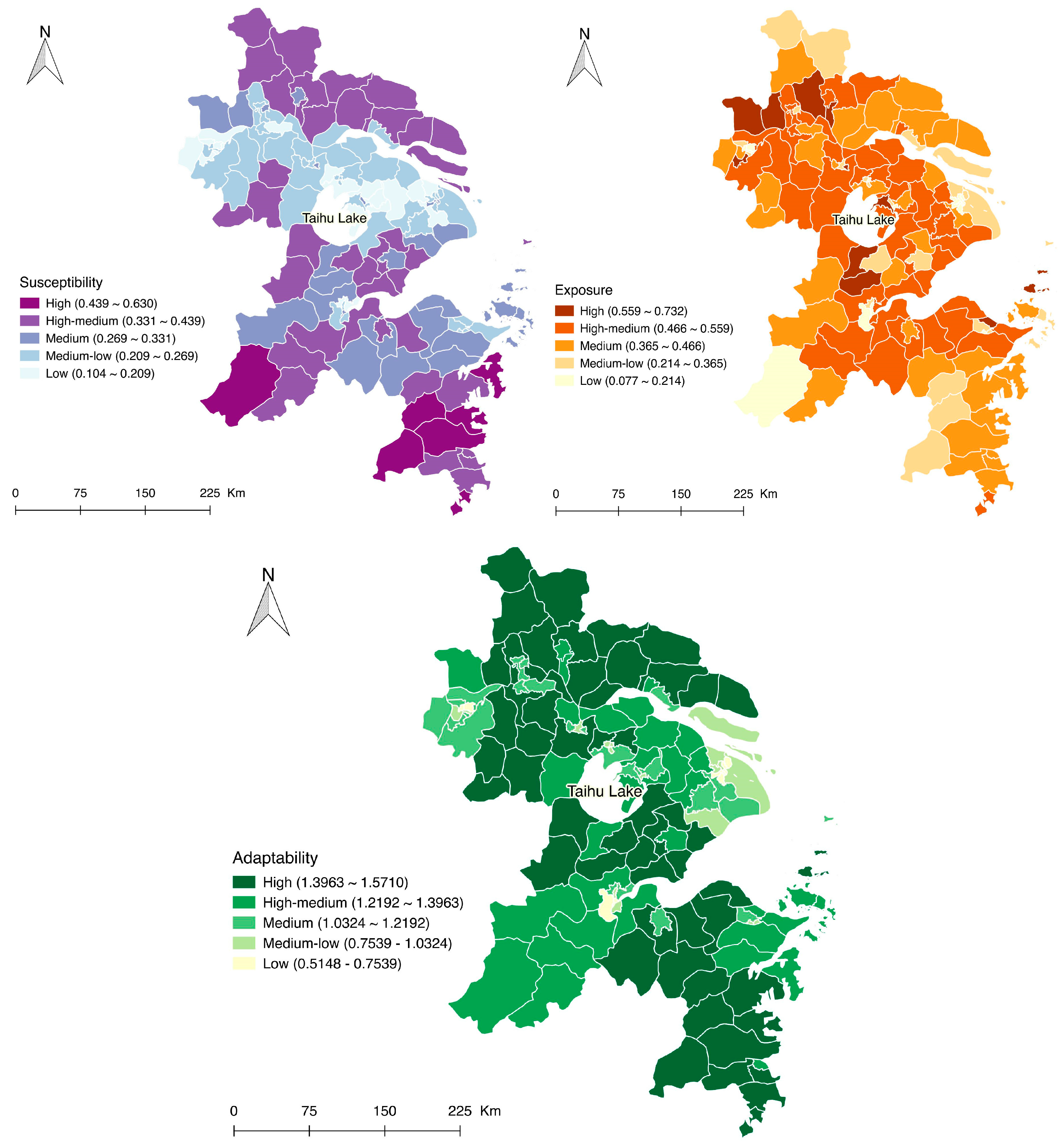
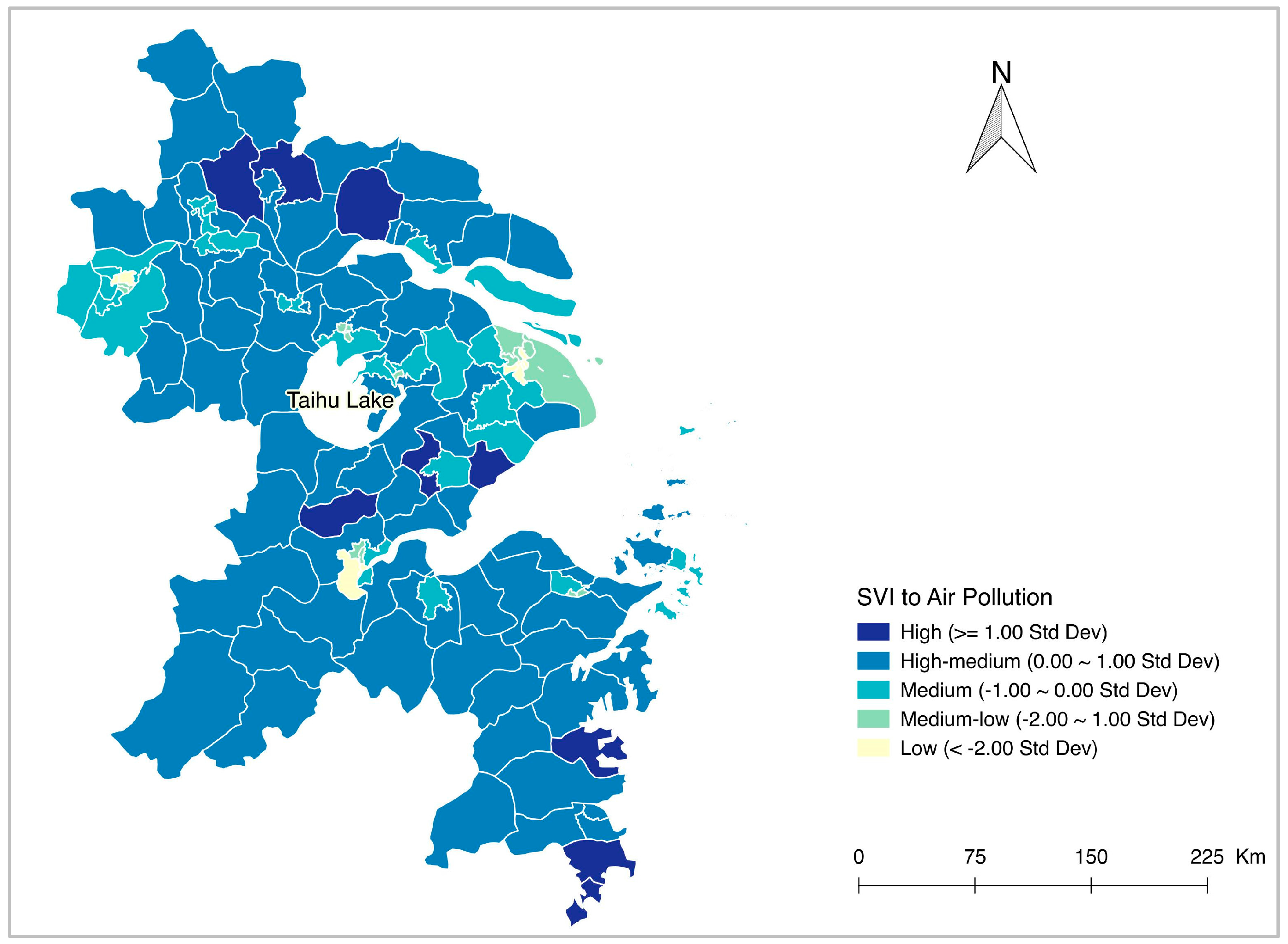
| High | 9 | 6.47% | 7 | 5.04% | 11 | 7.91% | 54 | 38.85% |
| High-medium | 75 | 53.96% | 39 | 28.06% | 50 | 35.97% | 32 | 23.02% |
| Medium | 30 | 21.58% | 28 | 20.14% | 36 | 25.90% | 25 | 17.99% |
| Medium-low | 15 | 10.79% | 47 | 33.81% | 24 | 17.27% | 17 | 12.23% |
| Low | 10 | 7.20% | 18 | 12.95% | 18 | 12.95% | 11 | 7.91% |
© 2017 by the authors; licensee MDPI, Basel, Switzerland. This article is an open access article distributed under the terms and conditions of the Creative Commons Attribution (CC-BY) license (http://creativecommons.org/licenses/by/4.0/).
Share and Cite
Ge, Y.; Zhang, H.; Dou, W.; Chen, W.; Liu, N.; Wang, Y.; Shi, Y.; Rao, W. Mapping Social Vulnerability to Air Pollution: A Case Study of the Yangtze River Delta Region, China. Sustainability 2017, 9, 109. https://doi.org/10.3390/su9010109
Ge Y, Zhang H, Dou W, Chen W, Liu N, Wang Y, Shi Y, Rao W. Mapping Social Vulnerability to Air Pollution: A Case Study of the Yangtze River Delta Region, China. Sustainability. 2017; 9(1):109. https://doi.org/10.3390/su9010109
Chicago/Turabian StyleGe, Yi, Haibo Zhang, Wen Dou, Wenfang Chen, Ning Liu, Yuan Wang, Yulin Shi, and Wenxin Rao. 2017. "Mapping Social Vulnerability to Air Pollution: A Case Study of the Yangtze River Delta Region, China" Sustainability 9, no. 1: 109. https://doi.org/10.3390/su9010109