Experimental Validation of a Wave Energy Converter Array Hydrodynamics Tool

Abstract

This paper uses experimental data to validate a wave energy converter (WEC) array hydrodynamics tool developed within the context of linearized potential flow theory. To this end, wave forces and power absorption by an array of five-point absorber WECs in monochromatic and panchromatic waves were measured from a set of deep-water wave basin experimental tests. Unlike the few other examples of WEC array experimental campaigns, the power take-off (PTO) system of each WEC was simulated by means of advanced equipment capable of accurately reproducing linear control strategies and, thereby, reducing the uncertainty in the physical model. Experimental measurements are then compared with numerical predictions showing reasonable agreement; the measured trends are, in the same way, well captured by the numerical predictions. Further analysis demonstrates that the developed tool can predict, on the safe side, wave forces and power absorption with less than 17.5% and 23.0% error, respectively, for more than 68% of the predictions.

1. Introduction

An increasing imbalance between the worldwide energy demand and the supply from fossil fuel and nuclear energy is expected during the next decades [1]. The gap between demand and supply is presumably to be covered by renewable energy sources, such as wind, solar and, among others, wave energy. However, there is still a long way to go before the renewable energy sector can overcome the imbalance between the projected energy demand and the non-renewable energy supply. Despite the current commercialization and continuous growth of installed electricity capacity from both wind and solar, the development of other renewable energies is still required in order to guarantee the supply of the future energy demand. Wave energy is, in this regard, an attractive source of energy as it is widespread, easily predictable and has huge potential; around 30–100 kW offshore wave power per unit width of wave front is estimated at latitudes within 40–50 degrees as averaged over the years [2]. This potential source of power has drawn the attention of many researchers since the early nineteenth century, which has currently led to a wide variety of WEC designs [3,4]; in Europe, however, it was after the oil crisis in 1973 that research and development of wave energy technologies experienced an increased support from governments and the private sector [5]. Nowadays, even though there are already wave energy developers who have been able to test their WECs in real sea conditions and to feed electricity to the grid [6], the wave technology has not yet progressed sufficiently in order to reach a commercialization stage. The high-cost of utility-scale wave power projects and the technical limitations, mainly associated with the installation and maintenance of WEC machines in such a harsh environment, are some of the reasons to the slow progress of the wave energy industry.

In order to reduce the costs of installation, operation, and maintenance, and to meet the demands of installed capacity, the deployment of WECs through arrays will be required. Arrays may consist from a few to hundreds of devices deployed in the same geographical location and systematically arranged in space through what is known as array layout, typically described as a set of rows and columns. As a result, the problem of finding the optimum array layout has been a major subject of debate [7,8,9,10,11,12,13]. The DTOcean (Optimal Design Tools for Ocean Energy Arrays) research project has developed open-source software [14] that addresses this problem in a novel way. While most commonly-used criteria to select optimal array layouts have been based on maximizing the energy production, the array layout solution of the DTOcean software comes from the minimization of the so-called levelized cost of energy (LCOE). This is defined as the ratio of the total life-cycle cost of the project divided by the annual energy production [15]. Therefore, besides the total energy output, the LCOE also accounts for installed capital cost, preventive maintenance and infrequent major overhauls together with some percentage valuation of the discount rate in order to arrive at a life-cycle. Hence, it appears to be a suitable metric to assess the optimality of the WEC array layout as it readily indicates competitiveness of electricity from WECs compared with other renewable electricity sources.

In the optimization routine, the LCOE, and so the energy production of the tentative WEC array solutions must be evaluated iteratively until a certain convergence criteria is met. Therefore, an accurate, but also computationally efficient, solver to calculate energy production of WEC arrays is required. A WEC array hydrodynamics tool [16] has been developed in this regard as a rational compromise between accuracy and computational effort. The accuracy level of the numerical model is given by the underlying linearized potential flow theory and the computational performance by the direct matrix method [17], which, for the sake of comparison, performs significantly faster than the widely-used boundary element method (BEM), especially for the solution of large arrays consisting of many WECs. The simplifying linearity assumption considered in the formulation of the model was motivated by the fact that waves in the sea are linear, i.e., small amplitude waves compared to the wave length and the water depth, for most of the time in a year, and so the annual energy production of the WEC array stems, to a large extent, from such linear waves. It is still a great concern whether or not the model is valid to accurately predict the energy absorbed by WEC arrays under the considered assumptions. Therefore, experimental testing constitutes a powerful tool for estimation of the uncertainty associated with the proposed model. Even though there are some examples of experimental testing of WEC arrays, such as the wave basin experiments carried out as part of the WECwakes project [18] or the experimental validation of the WEC array design and planning tools developed in the PerAWaT (Performance Assessment of Wave and Tidal array systems) project [19], the uncertainties introduced therein by the considered PTO mechanisms are seen as a major limitation for the data to be used.

The present study is devoted to the experimental validation and uncertainty assessment of the WEC array hydrodynamics tool implemented in the DTOcean open-source software. In order to validate the tool, wave forces and power absorption were measured from a set of wave basin experimental tests for a five-point absorber WEC array in monochromatic and panchromatic waves. Nonetheless, unlike in [18] and [19], the WECs were equipped with advanced PTO simulators capable of accurately generating linear loads (force directly proportional to velocity). Experimental measurements were then compared with numerical predictions in order to estimate the uncertainty in both wave forces and power absorption. In addition to the accuracy assessment of the numerical predictions, the uncertainty in wave forces may be used e.g. to estimate the structural reliability of the WECs [20,21] or to calibrate partial safety factors for WEC structures [22], whilst the uncertainty in power absorption allows, among other things, for further assessment of the LCOE in wave energy projects.

The work presented in this paper is structured in six sections. Section 2 provides the details of the point absorber WEC and the laboratory equipment of the experimental set-up. Section 3 describes the theoretical background that underpins the WEC array hydrodynamics tool and provides the basic equations to calculate the power absorption. Section 4 describes the design of the experimental tests and the methods used to derive wave forces and power absorption from both measurements and numerical predictions for each of the described tests. Section 5 defines the metrics used to assess the accuracy of predictions and the uncertainty in both wave forces and power absorption. Section 6 presents the comparison results and discusses the uncertainty in both wave forces and power absorption. Finally, Section 7 outlines the most relevant results obtained in this paper.

2. Physical Model

The physical model briefly described in this section is analogous to that described in [23,24], i.e., same WEC, PTO simulator, data acquisition equipment, and wave basin. The only difference between the physical model described here and the one in [23,24] is that, here, an array of WECs was modelled, whereas in [23,24] only a single WEC was modelled.

The WEC considered for the experiments was a small-scale version of one of the floaters of the Wavestar WEC [25]. This belongs to the point absorber category, which is designed to absorb energy from long-crested waves compared to their characteristic length, which, for the present WEC, corresponds to the buoy diameter. According to the prototype version of the Wavestar WEC installed in Hanstholm (Denmark), the WEC used in the experiments was reproduced at a scale 1:20 using Froude’s scaling law, i.e., units of length were multiplied by a factor 0.05 whereas units of time were multiplied by the squared root of that factor.

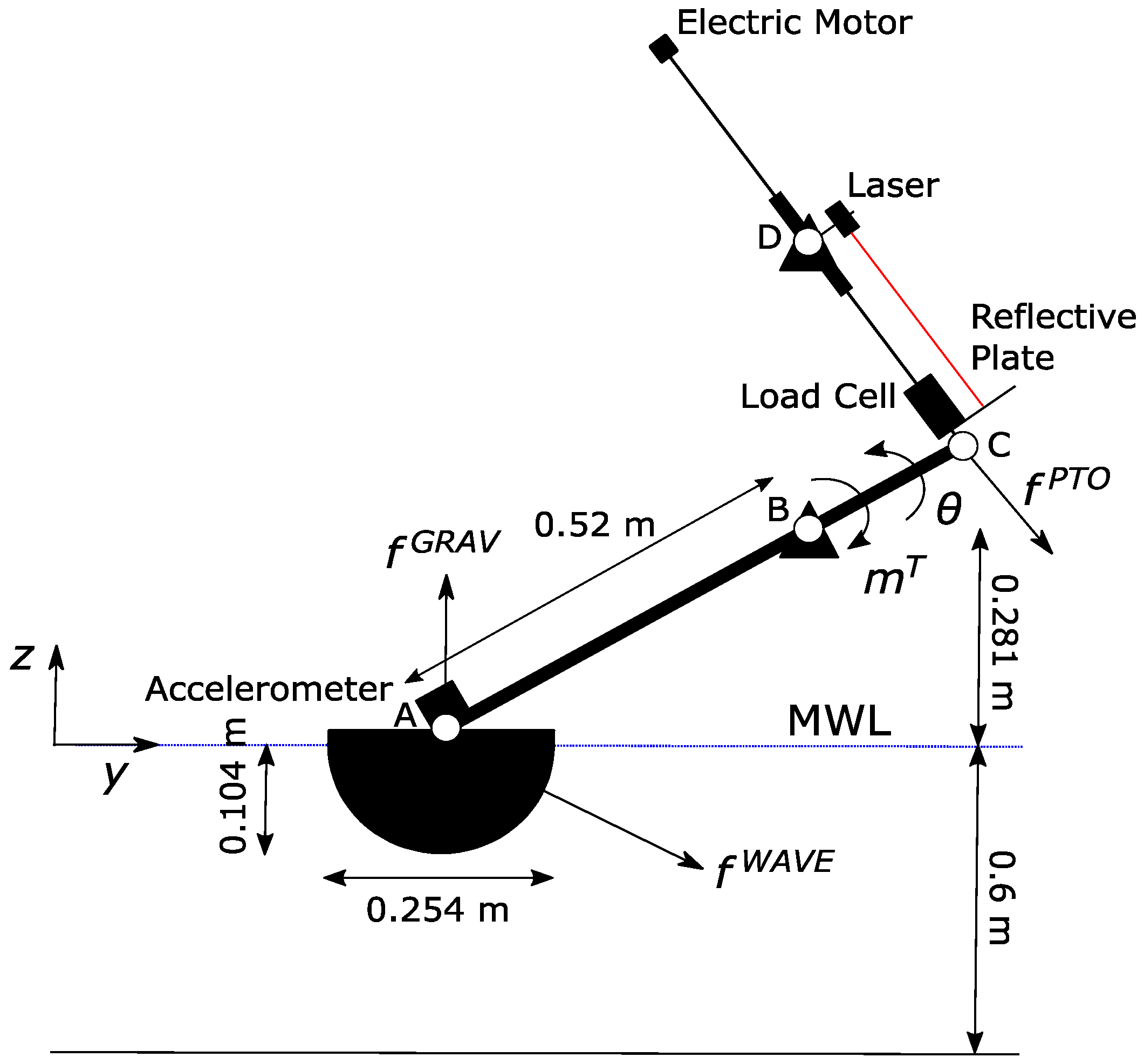
The WEC used in the experiments consisted of a semi-submerged buoy of 0.254 m diameter and 0.104 m draught connected to a 0.680 m long lever arm. The lever was hinged at 0.281 m high from the mean water level (MWL) allowing a rotation $\theta$ around the $x$-axis.

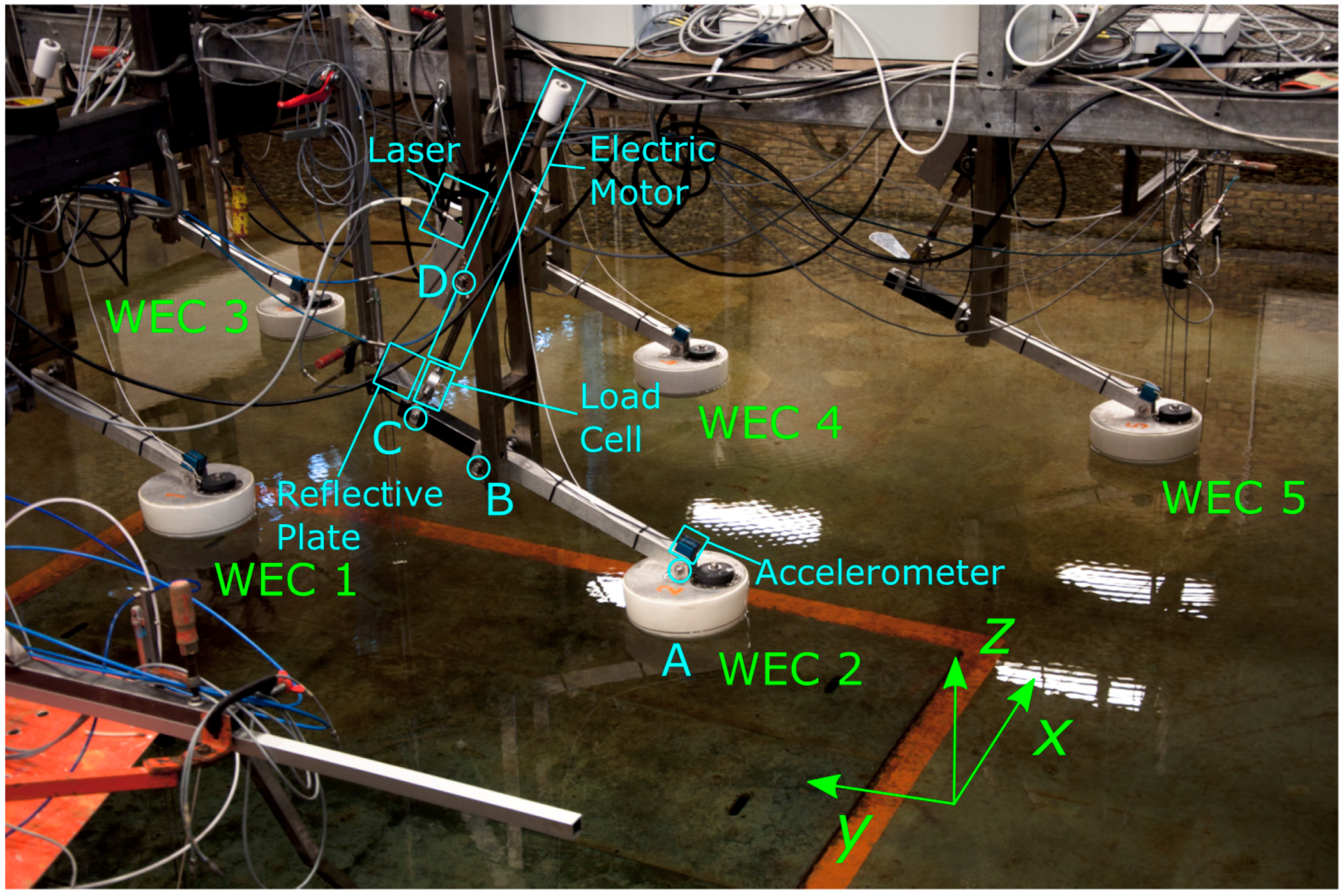
The WEC was equipped with a laser displacement sensor, Micro-Epsilon ILD-1402-600 (Micro-Epsilon, Ortenburg, Germany), and a reflective plate, from which one could record the changing distance between points $C$ and $D$ (Figure 1). The laser-plate system had been calibrated beforehand by testing the actual measurement with a set of known distances. Furthermore, an extension-compression s-beam load cell, Futek LSB302 (Futek, Irvine, CA, USA), was connected to the end extreme of the lever, point $C$, recording the force in the same direction as the segment $\overrightarrow{CD}$. The load cell was calibrated by testing the actual measurement with a set of known weights and assuming a linear relationship between the voltage signal and the output force. The two input signals, the changing distance $|\overrightarrow{CD}|$, and the force in the direction $\overrightarrow{CD}$, were recorded at a sample frequency of 200 Hz. Both signals, along with the known fixed distances $|\overrightarrow{BC}|$ and $|\overrightarrow{BD}|$, were further used to calculate the instantaneous rotation $\theta \left(t\right)$, with respect to the equilibrium floating position, and the instant resultant moment at the hinge $m^T\left(t\right)$. The angular acceleration $\ddot{\theta }\left(t\right)$ was deduced from the acceleration record of a dual-axis accelerometer ADXL203EB (Analog Devices, Norwood, MA, USA) installed at point $A$. Then, the angular velocity $\dot{\theta }\left(t\right)$ was derived from both the instantaneous rotation and angular acceleration by using a Kalman filter.

Figure 1 shows the equilibrium floating position of the WEC. The two triangles with an open dot, points $B$ and $D$, are vertically aligned, fixed in space, and they restrict motion so that only rotation in the plane of the figure is allowed. On the other hand, the open dots $A$ and $C$ allow for a relative rotation in the plane of the figure between buoy-lever and between lever-piston (thin line) respectively. The upper triangle, point $D$, incorporates a sliding bearing such that the laser is fixed in space while the piston passing through can slide back and forth.

In order to simulate the action of the PTO system, a piston was connected to the end extreme of the lever through the load cell and driven by an electric motor. The electric motor was a LinMot (NTI AG, Spreitenbach, Switzerland) linear motor of the P01-37x240 family controlled through a servo controller of the series LinMot E1100. The motor-controller system was calibrated through the LinMot-Talk 6.2 software, which assumes a linear relationship between the voltage signal and the output force. Then, a custom moment representing the action of the PTO system could be exerted at the hinge. However, errors between the target moment and the actual moment must be expected, mainly due to friction, which are undesirable from the control point of view. The LinMot servo controller integrates a proportional-integral control that accounts for the error made at the previous time (proportional) and the accumulated error (integral) in order to reduce the current error. The error was estimated as the difference between the target moment and the moment measured by the load cell signal.

In the laboratory, the PTO was required to behave as a linear damper, i.e., the moment exerted by the electric motor was targeted to be directly proportional to the angular velocity (see Section 3). Even though more sophisticated control strategies may be used to improve performance of WECs, the simple implementation of linear damping control makes it suitable for full scale WECs and also applicable to most WEC designs; therefore, it has been generally used in numerical models as the control strategy for a generic WEC and for WEC arrays, such as in [8,9,10,11,12,13] and in [16]. Additionally, and unlike other types of PTO systems, such as Coulomb dampers, linear dampers allow the physical model parameters and results to be scaled, as mentioned before, through Froude’s scaling law.

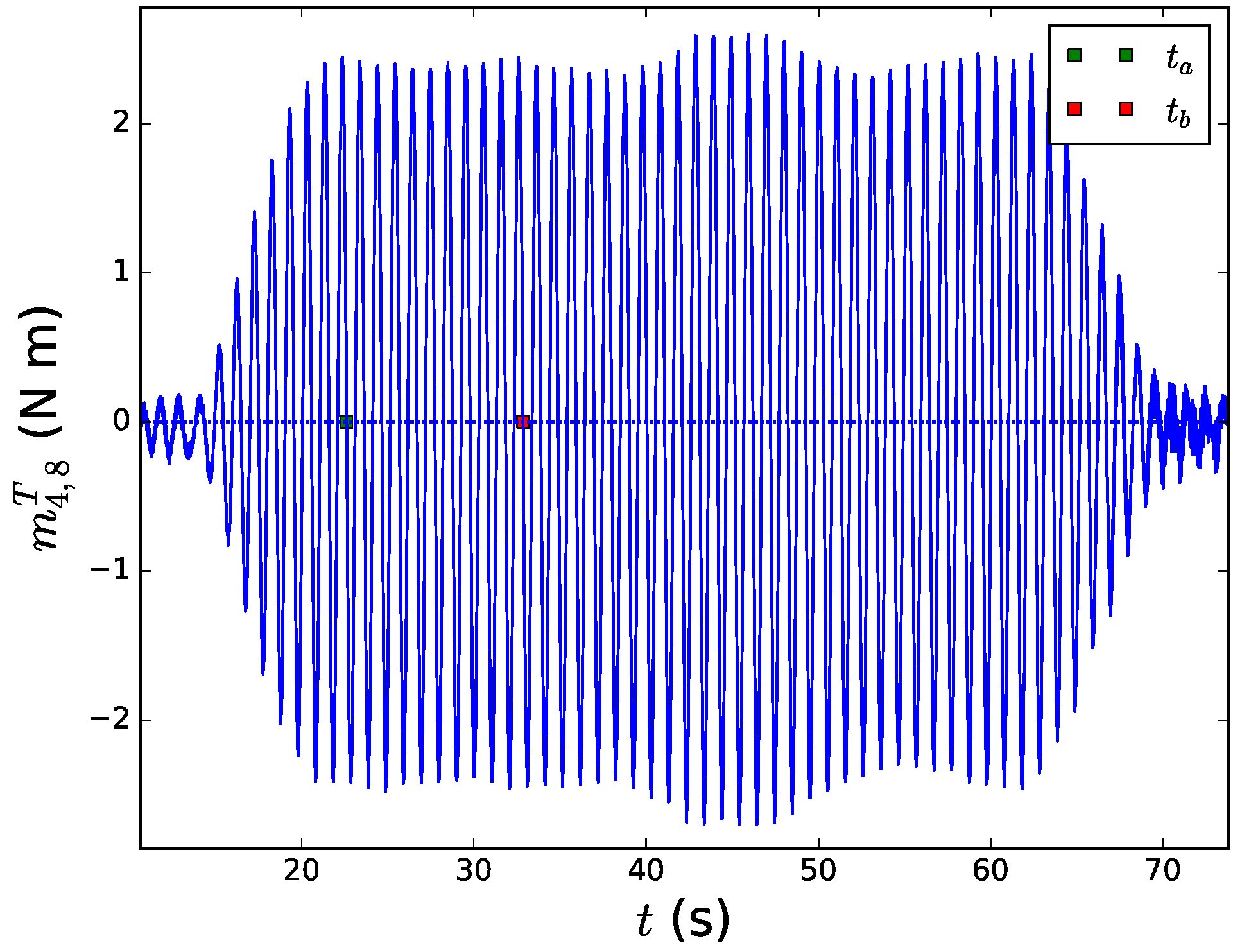
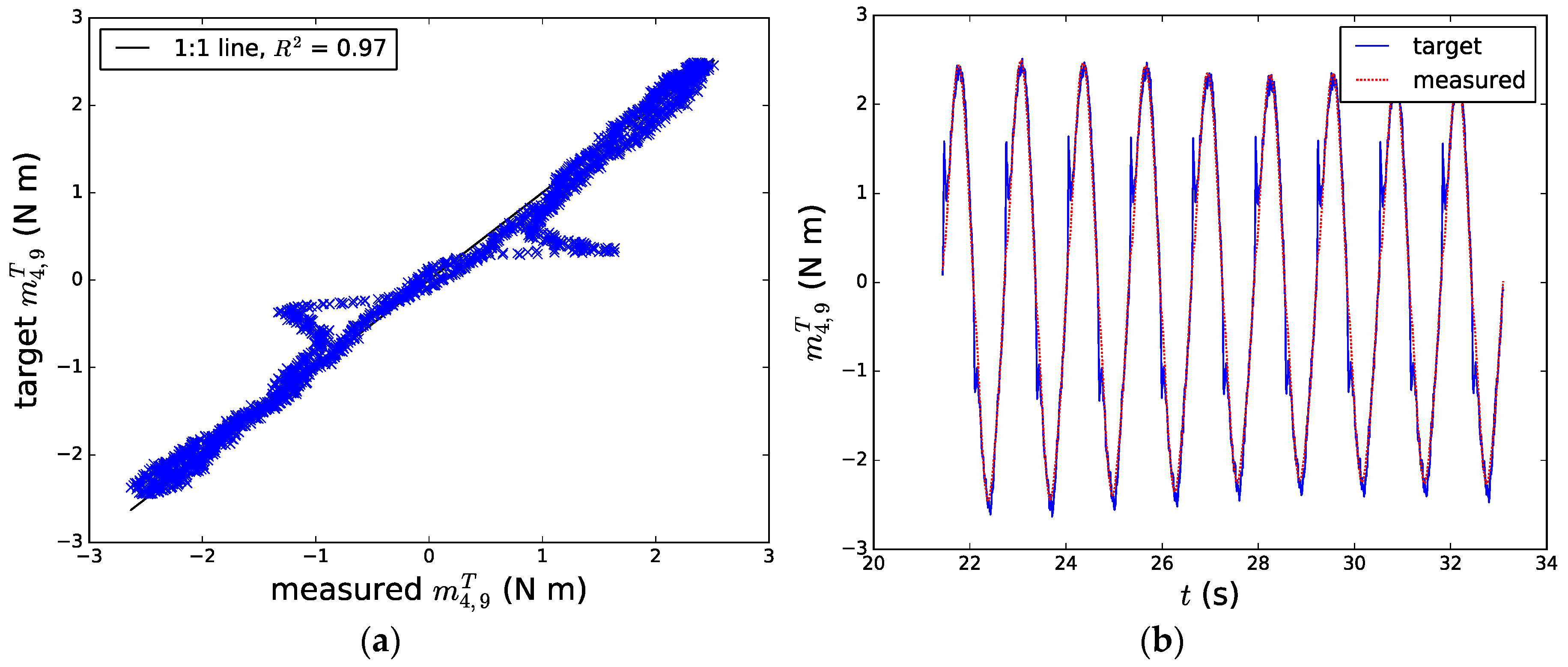
The accuracy of the motor-controller in reproducing the PTO linear behaviour is shown in Figure 2. The effect of the friction in the linear motor was observed to have a short duration; thus, having a negligible effect on the mean absorbed power (Equations (12) and (17)).

In addition to acting as a linear damper PTO, the motor-controller system was also used to induce a rotation to the WEC in the radiation test, as will be explained in Section 4.

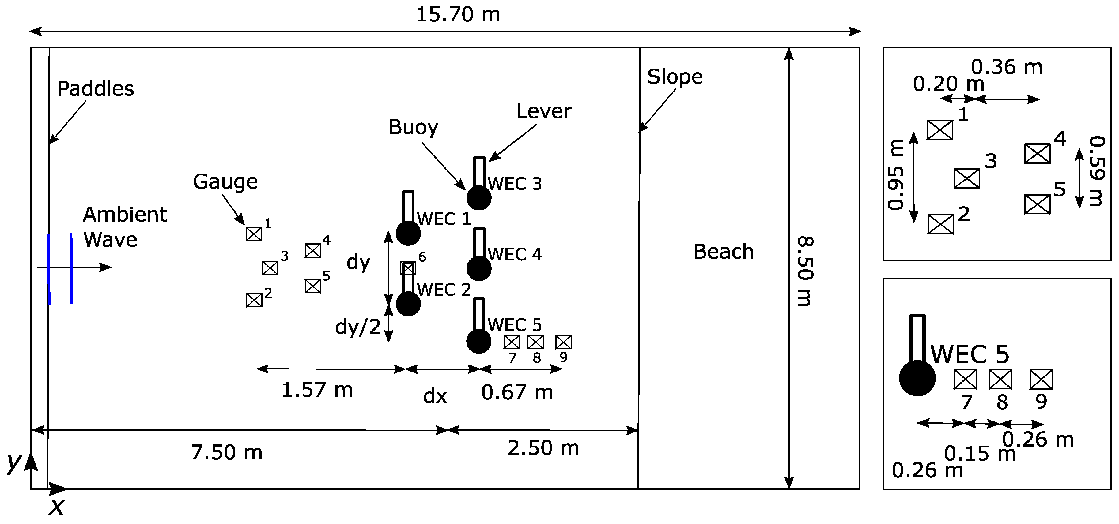
During the experimental campaign only a staggered array was considered with $dx=$ 1.28 m, $dy=$ 1.28 m, and a position shift along the $y$-axis of $dy/2$ between rows (Figure 3). Here, rows are the vertical lines drawn from the WECs sharing the same $x$-coordinate. The WEC array consisted of five WECs split into two rows consisting of two and three WECs, respectively.

The experiments were carried out in the deep-water wave basin at Aalborg University. The wave basin was 15.7 m long, 8.5 m wide, and had a water depth of 0.6 m. In order to minimize the effect of wave reflection, a gravel-type wave absorption beach was situated at the rear of the wave basin where the water depth decreased gradually from 0.6 m to 0 m along the $x$-direction. The wave basin was equipped with paddles that could generate long-crested plane waves travelling towards the $x$-direction only.

Moreover, in order to verify the amplitude and the period of the waves generated by the paddles, a set of five wave gauges measuring the free surface elevation were placed in front of the WEC array, and three behind WEC 5.

Figure 4 shows a picture of the experimental set-up in the deep-water wave basin at Aalborg University.

3. Numerical Model

The numerical model which underpins the WEC array hydrodynamics tool considered for the experimental validation was presented in [16]. Herein, the underlying assumptions, as well as the main equations to calculate the power absorption by the considered WEC array, are briefly explained.

The end goal of the numerical model is to predict the amount of wave power that will be absorbed by the WEC array. Considering the WECs are equipped with PTO systems that behave as standard linear dampers, the wave power absorbed by each WEC can be written as the product between the moment caused by the damper, denoted by $m^{PTO}$, and the angular velocity of the WEC:

$$\begin{array}{cc}{p}_i\left(t\right)=m_i^{PTO}\left(t\right){\dot{\theta }}_i\left(t\right)& i=1,\dots ,5\end{array},$$

(1)

where $m^{PTO}$ reads:

$$m_i^{PTO}\left(t\right)=-C^{PTO}{\dot{\theta }}_i\left(t\right);$$

(2)

and $C^{PTO}$ is the corresponding linear damping coefficient which, for the sake of simplicity, is the same for all WECs.

Therefore, before the estimation of the absorbed power through Equation (1), one must first solve the motion of the WECs. To this end, Newton’s second law is applied under the following considerations:

• The forces acting on the WECs are mainly due to the wave-WECs interaction, the action of gravity, and the PTO system ($f^{WAVE}$, $f^{GRAV}$, and $f^{PTO}$ in Figure 1).
• The wave-WECs interaction forces are derived within the context of linearized potential flow theory and constant water depth.
• The ambient wave is a monochromatic plane wave of unit amplitude and wave angular frequency $\omega$.
• The time variation is harmonic: $q(t)=\Re (\tilde{Q}(\omega )e^{\tilde{i}\omega t})$, where $q$ is any time-dependent physical quantity, $\tilde{Q}$ the associated frequency-dependent complex amplitude, and $\tilde{i}=\sqrt{-1}$.

Then, the equation of motion at the hinge for each WEC in the frequency domain due to the excitation caused by a unit amplitude wave with wave frequency $\omega$ reads:

$${{\displaystyle \sum }}_{j=1}^5\left(-{\omega }^2\left(I{\delta }_{ij}+I_{ij}^R\left(\omega \right)\right)+\tilde{i}\omega \left(C^{PTO}{\delta }_{ij}+C_{ij}^R\left(\omega \right)\right)+K{\delta }_{ij}\right){\tilde{\Theta }}_j\left(\omega \right)={\tilde{M}}_i^D\left(\omega \right),$$

(3)

where $\delta$ is the Kronecker Delta, $\tilde{\Theta }$ is the complex amplitude of the rotation, ${\tilde{M}}^D$ the complex amplitude of the diffraction moment, $I^R$ the added mass matrix, $C^R$ the radiation damping matrix, $I=$ 0.778 kg m²/rad is the moment of inertia coefficient, and $K=$ 87 N m/rad is the hydrostatic stiffness coefficient.

The forces caused by the wave-WECs interaction, herein also called wave forces, are the diffraction moment ${\tilde{M}}^D$ and the radiation moment ${\tilde{M}}^R=\left({\omega }^2{I}^R-\tilde{i}\omega C^R\right)$. These are defined per unit amplitude wave and rotation, respectively. The wave forces are herein solved using the so-called direct matrix method [17], which tends to be computationally faster than standard BEM techniques. Existing literature, such as [26], already proves its efficiency and accuracy when compared with commercially available BEM solvers. However, the method requires the solution of the hydrodynamic problem for one isolated WEC, which, in the present numerical model, is done through the open-source BEM software Nemoh [27]. Thereafter, the hydrodynamic problem for the interacting WECs can be solved through [17] for any number of WECs and configurations.

The instant resultant moment defined in Section 2, taking into account the assumptions listed above, is calculated per unit amplitude wave as:

$$m_i^T\left(t\right)=\Re \left(\left({{\displaystyle \sum }}_{j=1}^5\left(-{\omega }^2\left(I{\delta }_{ij}+I_{ij}^R\left(\omega \right)\right)+\tilde{i}\omega C_{ij}^R\left(\omega \right)+K{\delta }_{ij}\right){\tilde{\Theta }}_j\left(\omega \right)-{\tilde{M}}_i^D\left(\omega \right)\right)e^{\tilde{i}\omega t}\right),$$

(4)

In the numerical model presented in this section, neither the wave basin vertical walls nor the beach are taken into account. Therefore, the present numerical model is indeed meant for open-sea conditions rather than wave basin conditions, and so this will invariably be a source of error.

In order to show the efficiency of the numerical model, the wall-clock time elapsed to produce the absorbed power by the WEC array for all of the wave conditions listed in

Table 2. Panchromatic wave details.

ID Number, $\mathit{u}$ (#)	Peak Period, ${\mathit{T}}_{\mathit{P}}$ (s)	Peak Frequency, ${\mathbf{\omega }}_{\mathit{P}}$ (rad/s)	Significant Wave Height, ${\mathit{H}}_{\mathit{s}}$ (cm)	Wave Direction (degrees)	Experiment Duration, $\mathit{\tau }$ (s)
1	1.421	4.422	6.000	0.000	143.080
2	1.191	5.276	6.000	0.000	114.070
3	1.025	6.130	4.500	0.000	97.600
4	0.900	6.981	4.500	0.000	85.410
5	0.848	7.410	4.500	0.000	80.390

was measured. Using an Intel^® Core™ i7-4800MQ (Intel Corporation, Santa Clara, CA, USA) processor with base frequency 2.70 GHz, the mean elapsed time after 100 runs was 0.074 s.

4. Design of Experiments

Three different types of tests were run: diffraction, radiation, and power absorption tests; the first two were designed to validate wave forces, whereas the last was meant to validate the power absorption.

Predicted and measured resultant moment amplitude, denoted by ${\widehat{M}}^T$ and $M^T$, respectively, were then compared in both diffraction and radiation tests, whereas predicted and measured mean absorbed power, denoted by $\widehat{\overline{p}}$ and $\overline{p}$, respectively, were compared in the power absorption test.

4.1. Wave Forces: Diffraction Test

In the diffraction test, all five WECs were fixed at their equilibrium floating position while excited by a monochromatic plane wave, which can be represented by an oscillation of the free surface elevation:

$${\eta }^M\left(x,t\right)=A\cos \left(\omega t-kx\right),$$

(5)

with amplitude $A=H/2$ (

Table 1. WEC motion and monochromatic wave details.

ID Number, $\mathit{l}$ (#)	Period (s)	Angular Frequency, $\mathit{\omega }$ (rad/s)	Wave Height, $\mathit{H}$ (cm) 1	Wave Direction (degrees) 1	Rotation Amplitude, ${\mathit{\Theta }}_4$ (rad) 2
1	2.000	3.142	4.500	0.000	0.100
2	1.761	3.568	4.500	0.000	0.100
3	1.573	3.994	4.500	0.000	0.100
4	1.421	4.422	4.500	0.000	0.100
5	1.296	4.848	4.500	0.000	0.100
6	1.191	5.276	4.500	0.000	0.100
7	1.102	5.702	4.500	0.000	0.100
8	1.025	6.130	4.500	0.000	0.100
9	0.959	6.552	4.500	0.000	0.100
10	0.900	6.981	4.500	0.000	0.100
11	0.848	7.410	4.500	0.000	0.100
12	0.802	7.834	4.500	0.000	0.100
13	0.761	8.256	4.500	0.000	0.100

Notes: ¹ Only diffraction and power absorption tests and ² only radiation tests.

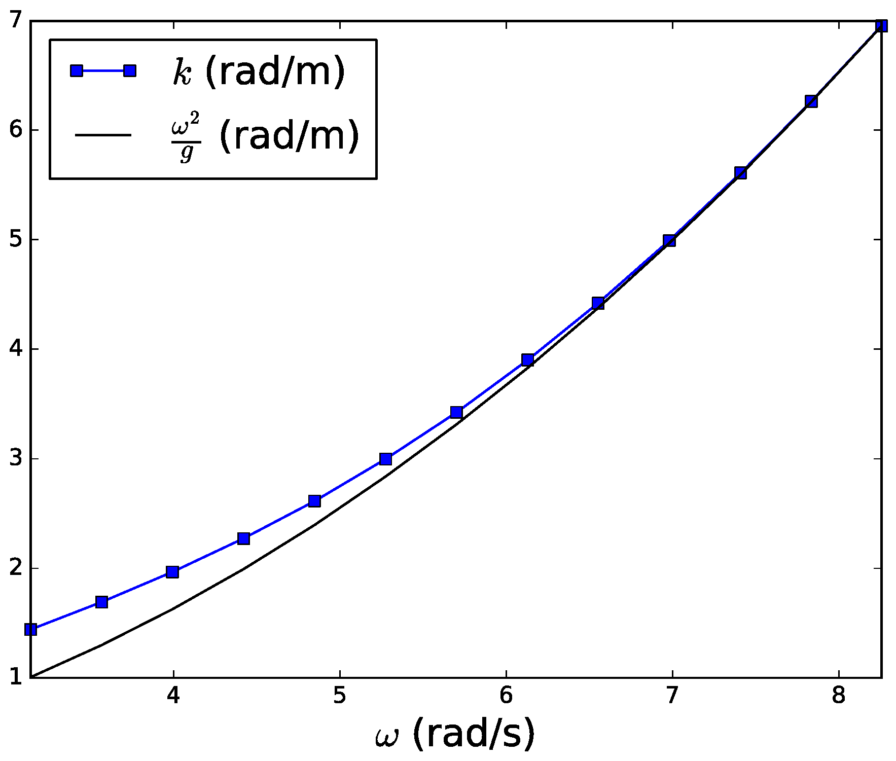
) and wavenumber $k$, which is defined as the root of the dispersion equation:

$$k\tanh kh={\omega }^2/g,$$

(6)

where $g$ is the acceleration due to gravity and $h=$ 0.6 m the water depth. As the wave frequency increases, the wavenumber can be approximated to ${\omega }^2/g$. This is usually interpreted as the sea-bottom having no effect on the wave. The wave is then referred to as a deep-water wave and can be accurately modelled as a linear wave. This is illustrated in Figure 5 for the wave conditions reported in Table 1.

The physical model and the numerical model were run by generating one monochromatic wave, with associated angular frequency ${\omega }_l$ (Table 1), at a time and without repetition.

In the physical model, the instant resultant moment was derived from the load cell signal as described in Section 2. Then, in order to calculate the amplitude of the moment from the time series, a time interval $\left[t_a,t_b\right]$ was first selected as the earliest part of the record where the amplitude of the oscillations was observed to remain constant. The earliest part was chosen so that the reflections caused by the presence of the vertical lateral walls and the beach had the smallest effect, while approximately ten consecutive oscillations of similar amplitude was decided sufficient to ensure the amplitude was stationary (see Figure 6). Finally, the Fourier transform of the selected time record was done:

$$M_{il}^T=\left|\frac{2}{{t_b}_{il}-{t_a}_{il}}{{\displaystyle \int }}_{{t_a}_{il}}^{{t_b}_{il}}{m}_{il}^T\left(t\right)e^{-\tilde{i}{\omega }_l\left(t-{t_a}_{il}\right)}dt\right|/A.$$

(7)

Equation (7) provides the measured resultant moment amplitude per unit amplitude wave.

The resultant moment amplitude predicted by the numerical model is indeed the diffraction moment (see Equation (4)), which was already defined per unit amplitude wave:

$${\widehat{M}}_{il}^T=\left|{\tilde{M}}_i^D\left({\omega }_l\right)\right|.$$

(8)

4.2. Wave Forces: Radiation Test

In the radiation test, the WEC 4 was forced to oscillate, approximately 20 oscillations, through:

$${\theta }_4\left(t\right)={\Theta }_4\cos \left(\omega t\right),$$

(9)

with a rotation amplitude ${\Theta }_4=$ 0.10 rad (Table 1), while the rest of the WECs were fixed at their equilibrium floating positions.

Since the amplitude of radiated waves decay proportionally to one divided by the squared root of the distance from the WEC where they were generated, the WEC closest to the centre of the array was expected to have the greatest impact on the rest of the WECs. Larger amplitudes are desirable for the quality of the measured data; therefore, WEC 4 was selected to radiate waves in the radiation test.

The physical model and the numerical model were run by making the WEC 4 oscillate according to Equation (9) with one oscillation frequency ${\omega }_l$ (Table 1) at a time and without repetition.

The same procedure used to obtain the resultant moment amplitude in the diffraction test was used again in the radiation test:

$$M_{il}^T=\left|\frac{2}{{t_b}_{il}-{t_a}_{il}}{{\displaystyle \int }}_{{t_a}_{il}}^{{t_b}_{il}}{m}_{il}^T\left(t\right)e^{-\tilde{i}{\omega }_l\left(t-{t_a}_{il}\right)}dt\right|/{\Theta }_4,$$

(10)

although the resultant moment amplitude is given per unit amplitude rotation.

The resultant moment amplitude predicted by the numerical model is the radiation moment for all fixed WECs, whereas the effect of the rotational inertia and the restoring hydrostatic moment must be added for the moving WEC (see Equation (4)):

$${\widehat{M}}_{il}^T=\left|-{\omega }_l^2\left(I{\delta }_{i4}+I_{i4}^R\left({\omega }_l\right)\right)+\tilde{i}{\omega }_l{C}_{i4}^R\left({\omega }_l\right)+K{\delta }_{i4}\right|.$$

(11)

The resultant moment amplitude in Equation (11) was already defined per unit amplitude rotation.

4.3. Power Absorption Test

The power absorption test was meant to reproduce the WEC array in its normal operation conditions. Thus, the WECs were floating and exposed to the action of linear damping PTO systems, with a $C^{PTO}=10$ N m s/rad, while excited by two different sets of waves: monochromatic (Table 1), with the same amplitude as in the diffraction test; and panchromatic waves (Table 2).

In the physical model, the linear damping PTO effect was accomplished by exerting an instantaneous force through the piston so that this was targeted to yield a moment at the hinge, the same as in Equation (2), but substituting $\dot{\theta }$ by the measured instant angular velocity. Therefore, the measured resultant moment for the power absorption test is indeed the moment caused by the action of the piston and so it should be roughly the same as the targeted one (Figure 2). At this point, the advanced capabilities of the PTO simulators used during the experimental campaign played such an important role in order to accurately generate the target moment.

The physical model and the numerical model were run by generating one monochromatic wave, with associated angular frequency ${\omega }_l$ (Table 1), at a time and without repetition.

In the physical model, the mean absorbed power for monochromatic waves was computed by first selecting a time interval $\left[t_a,t_b\right]$ in the same way as in the diffraction test. Finally, the measured resultant moment and the measured angular velocity were substituted into Equation (1) and the result was averaged throughout the selected time interval:

$${\overline{p}}_{il}=\left(\frac{1}{{t_b}_l-{t_a}_l}{{\displaystyle \int }}_{{t_a}_l}^{{t_b}_l}{m}_{il}^T\left(t\right){\dot{\theta }}_{il}\left(t\right)dt\right)/\overline{P}\left({\omega }_l\right).$$

(12)

Equation (12) provides the so-called capture factor, which is defined as the ratio of the measured mean absorbed power divided by the mean incident wave power along the width equivalent to the buoy diameter $D=0.254$ m:

$$\overline{P}=D\frac{\rho g^2}{4}\frac{A^2}{\omega }$$

(13)

where $\rho$ is the water density.

The predicted mean absorbed power was computed by averaging the absorbed power from Equation (1) throughout a wave period and multiplied by the squared amplitude wave:

$${\widehat{\overline{p}}}_{il}=\frac{1}{2}{\omega }_l^2{C}^{PTO}{\left|{\tilde{\Theta }}_i\left({\omega }_l\right)\right|}^2{A}^2/\overline{P}\left({\omega }_l\right),$$

(14)

where the rotation amplitude is defined per unit amplitude wave.

Panchromatic waves are of particular interest as they provide a better approximation to real sea state conditions than monochromatic waves. The vertical variation of the free surface for the panchromatic waves can be written as:

$${\eta }^P\left(x,t\right)={{\displaystyle \sum }}_{n=1}^{\infty }A\left({\omega }_n\right)\cos \left({\omega }_{n}t-k_{n}x\right),$$

(15)

where the amplitude of each monochromatic wave is herein calculated from the JONSWAP spectrum with a peak enhancement factor $\gamma =3.3$:

$$S\left(T_p,H_s,\omega \right)=\frac{1}{2}\frac{A^2}{\Delta \omega },$$

(16)

The physical model and the numerical model were run by generating one panchromatic wave (Table 2) at a time and without repetition.

The measured mean absorbed power from panchromatic waves was calculated the same way as for monochromatic waves although averaging throughout the entire time record (Table 2):

$${\overline{p}}_{iu}=\left(\frac{1}{{\tau }_u}{{\displaystyle \int }}_0^{{\tau }_u}{m}_{iu}^T\left(t\right){\dot{\theta }}_{iu}\left(t\right)dt\right)/\overline{P^{*}}\left({\left(T_p,H_s\right)}_u,\omega \right),$$

(17)

Equation (17) provides the capture factor for panchromatic waves. Here, the mean incident wave power along the width equivalent to the buoy diameter reads:

$$\overline{P^{*}}=D\frac{\rho g^2}{4}{{\displaystyle \int }}_0^{\infty }\frac{1}{\omega }2S\left(T_p,H_s,\omega \right)d\omega .$$

(18)

Equation (18) for deep water assumption turns into the commonly used:

$$\overline{P^{*}}=D\frac{\rho g^2}{64\pi }{H}_{m0}^2{T}_e,$$

(19)

with $H_{m0}$ being the spectral significant wave height and $T_e$ the energy period.

The predicted mean absorbed power was computed as a weighted sum of mean absorbed power from monochromatic waves, with the weights being the corresponding spectral values:

$${\widehat{\overline{p}}}_{iu}=\left({{\displaystyle \int }}_0^{\infty }2S\left({\left(T_p,H_s\right)}_u,\omega \right){\omega }^2{C}^{PTO}{\left|{\tilde{\Theta }}_i\left(\omega \right)\right|}^{2}d\omega \right)/\overline{P^{*}}\left({\left(T_p,H_s\right)}_u,\omega \right).$$

(20)

5. Prediction Errors

In order to study the accuracy of the numerical model predictions for each experimental test and for each WEC, the mean absolute percentage error (MAPE) is used:

$${\mathrm{MAPE}}_i=\frac{1}{13}{{\displaystyle \sum }}_{l=1}^{13}\left|\frac{\left({\widehat{M}}_{il}^T-M_{il}^T\right)}{M_{il}^T}\right|\times 100,$$

(21)

for diffraction and radiation tests;

$${\mathrm{MAPE}}_i=\frac{1}{13}{{\displaystyle \sum }}_{l=1}^{13}\left|\frac{\left({\widehat{\overline{p}}}_{il}-{\overline{p}}_{il}\right)}{{\overline{p}}_{il}}\right|\times 100,$$

(22)

for the power absorption test when monochromatic waves are considered; and:

$${\mathrm{MAPE}}_i=\frac{1}{5}{{\displaystyle \sum }}_{u=1}^5\left|\frac{\left({\widehat{\overline{p}}}_{iu}-{\overline{p}}_{iu}\right)}{{\overline{p}}_{iu}}\right|\times 100,$$

(23)

when panchromatic waves are considered.

Finally, the uncertainty in both wave forces and power absorption is assessed through the mean and the standard deviation of the percentage error $ϵ$:

$$ϵ=\frac{{\widehat{M}}^T-M^T}{M^T}\times 100,$$

(24)

for diffraction and radiation tests; and:

$$ϵ=\frac{\widehat{\overline{p}}-\overline{p}}{\overline{p}}\times 100,$$

(25)

for the power absorption test.

A total of 130 percentage error values are used for the wave forces uncertainty assessment (Equation (24)); while a total of 90 percentage error values are used for the power absorption uncertainty assessment (Equation (25)).

6. Results and Discussion

Firstly, the accuracy of the physical model in reproducing the wave conditions designed for the tests (Table 1 and Table 2) is assessed. Secondly, the predictions made by the numerical model are graphically compared with the experimental measurements. Finally, the MAPE, the mean percentage error, and the standard deviation of the percentage error are reported and discussed.

The layout of subplots in Figures 8–11 follows the same staggered layout as the physical array layout described in Section 2. Therefore, the direction of propagation of the incident waves corresponds to the $x$-axis, from left-to right, of Figures 8–11.

Even though the array layout and the incident waves are symmetric with respect to the $x$-axis, there is no such axis of symmetry for the WEC array (see Figure 3 and Figure 4). Therefore, the results presented in Figures 8–11 are not expected to be symmetric with respect to the $x$-axis.

The uncertainty on the measured data due to the uncertainty on the generated waves (Section 6.1) is depicted in Figures 7–11 as a grey shaded area. The limits of the area are set so that it spans $\pm$ two standard deviations from the mean measured data (red dots).

6.1. Uncertainty on the Generated Wavefield

Before carrying out the diffraction and the power absorption tests, the set of monochromatic waves in Table 1 and the set of panchromatic waves in Table 2 were generated in the wave basin without the WEC array. Three and two repetitions were carried out for each monochromatic and panchromatic wave, respectively. The waves were then measured at different locations through the set of wave gauges shown in Figure 3. However, wave gauges 7–9 were only used in one of the repeats.

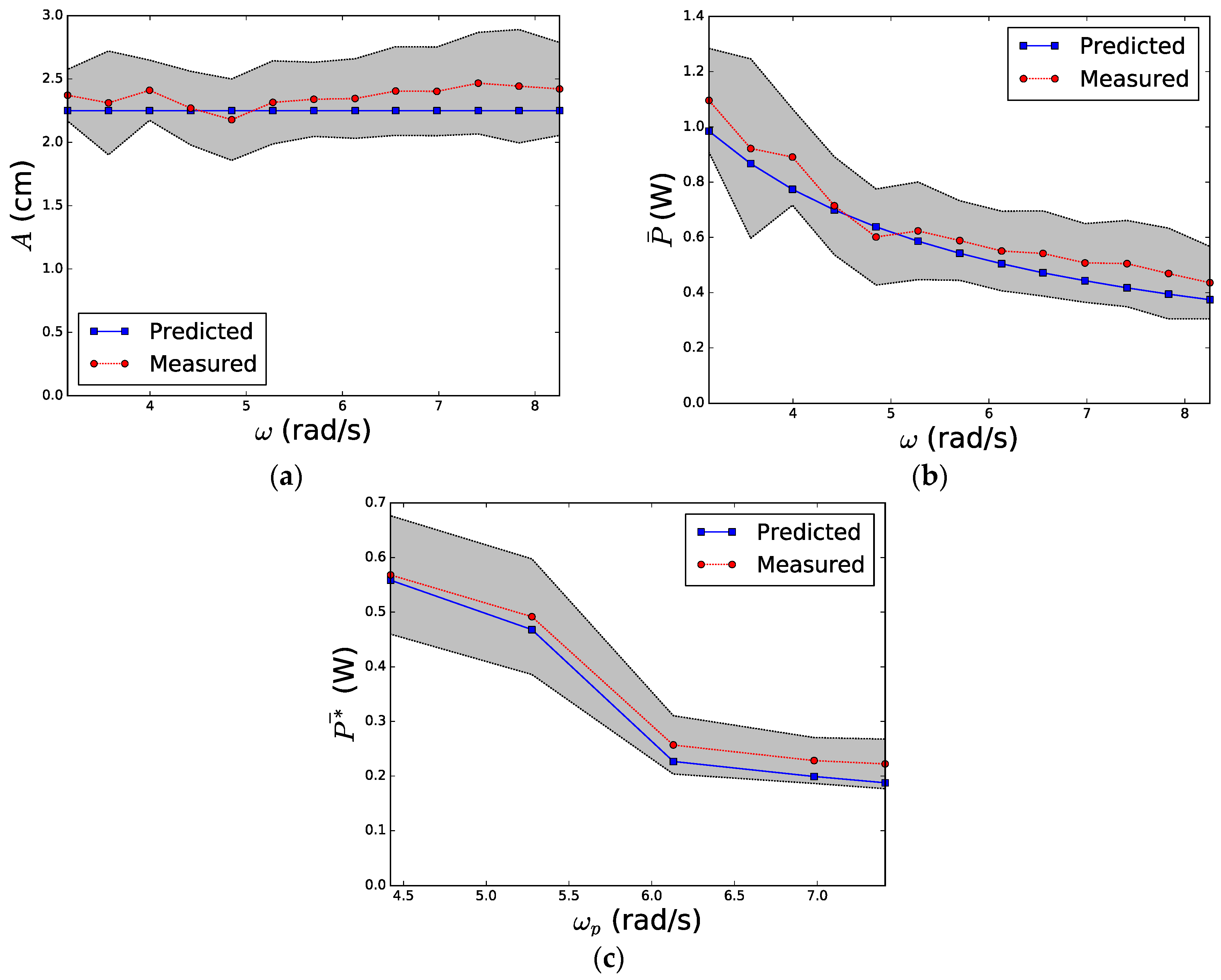
The free surface elevation values measured by the wave gauges were further used to calculate the wave amplitude in Equation (7) and the incident wave power in Equations (12) and (17). These are shown in Figure 7 (red line) together with the target values (blue line). Regarding the incident wave power in monochromatic waves, it was proportional to the squared wave amplitude and proportional to the wave period (Equation (13)); thus, Figure 7a and Figure 7b are linked in this same way.

The deviation between the target and measured wave parameters was mainly associated to the differences from the record of one wave gauge to another rather than from one repeat to another. Nevertheless, the number of different wave gauges was also much larger than the number of repetitions. Thus, no distinction was made on the source of the uncertainty when assessing the uncertainty on the generated waves.

With regard to the measured wave angular frequencies, these matched the target ones perfectly. In panchromatic sea states, the shape of the corresponding spectrum was also well captured by the measurements.

Overall, the maximum standard deviation encountered was 0.22 cm, 0.16 W, and 0.05 W for the wave amplitude, mean incident wave power in monochromatic waves, and panchromatic waves, respectively. Thus, the standard deviation for the measured wave parameters can be seen to be bounded by approximately 10% of the target value.

6.2. Wave Forces: Diffraction Test

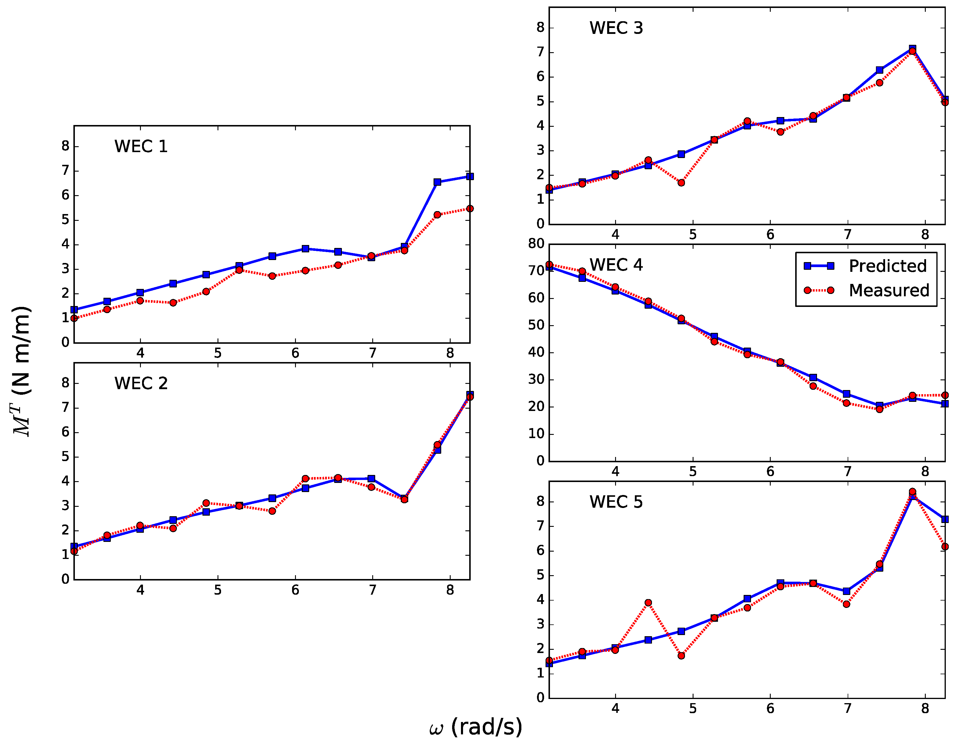
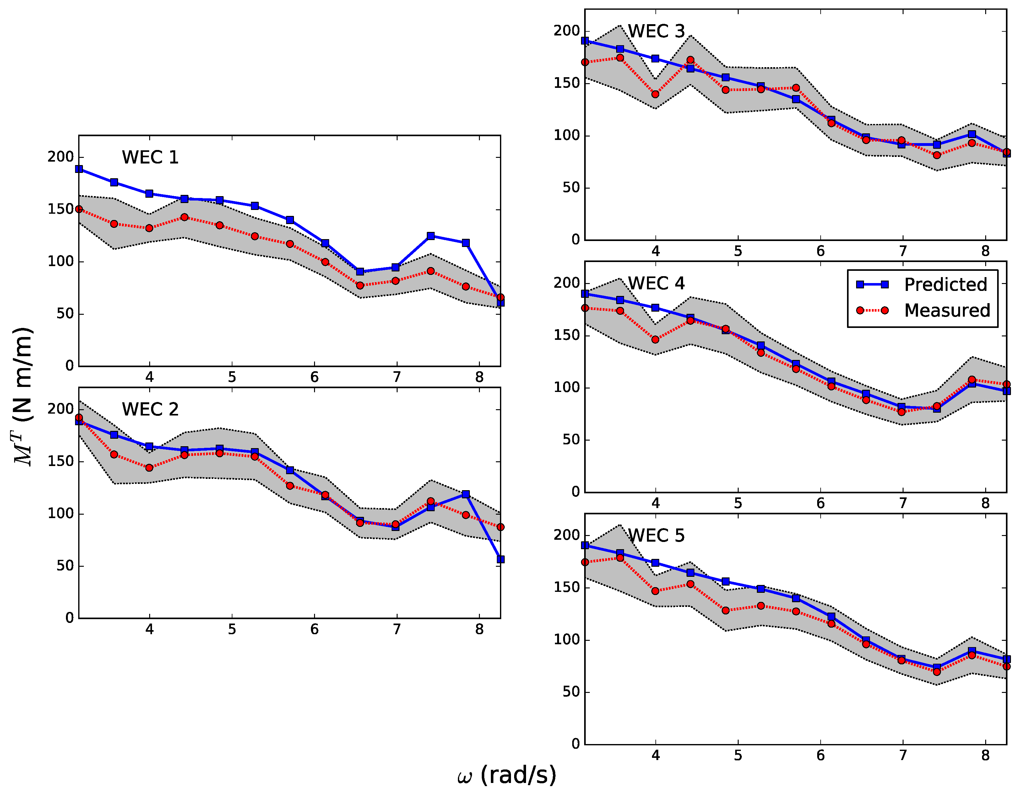
Figure 8 shows the predicted (blue line) and measured (red line) resultant moment amplitude for the diffraction test and for each WEC. The first is obtained through Equation (8) and the second through Equation (7).

The agreement between predictions and measurements is generally good, and the measured trend is also well captured by the numerical results; however, the predicted resultant moment amplitude is clearly larger than the measured one for the WEC 1. This inconsistency is only partially covered by taking into account the uncertainty of the measured wave amplitude discussed in the previous section (grey region), and so the largest expected moment amplitude yielded from measurements is still smaller than the predictions made by the numerical model.

Overall, the numerical model in the diffraction test is seen to predict the resultant moment amplitude with reasonable accuracy. The maximum deviation shown in Figure 8 for the measured data corresponds to approximately $\pm$20% the mean value (red dots).

6.3. Wave Forces: Radiation Test

Figure 9 shows the predicted (blue line) and measured (red line) resultant moment amplitude for the radiation test and for each WEC. The first is obtained through Equation (11) and the second through Equation (10).

As in the diffraction test, the numerical model matches the general trend from the measured resultant moment amplitude; besides, the agreement between measurements and predictions for the moving WEC 4 is excellent. The inconsistency in the prediction for the WEC 1 seems to be less important than in the diffraction test, although it is still persistent. Overall, apart from the few disagreements that can be seen for WEC 3 and 5 at the frequency range between 4 and 5 rad/s, the performance of the numerical model is, again, satisfactory.

6.4. Power Absorption Test

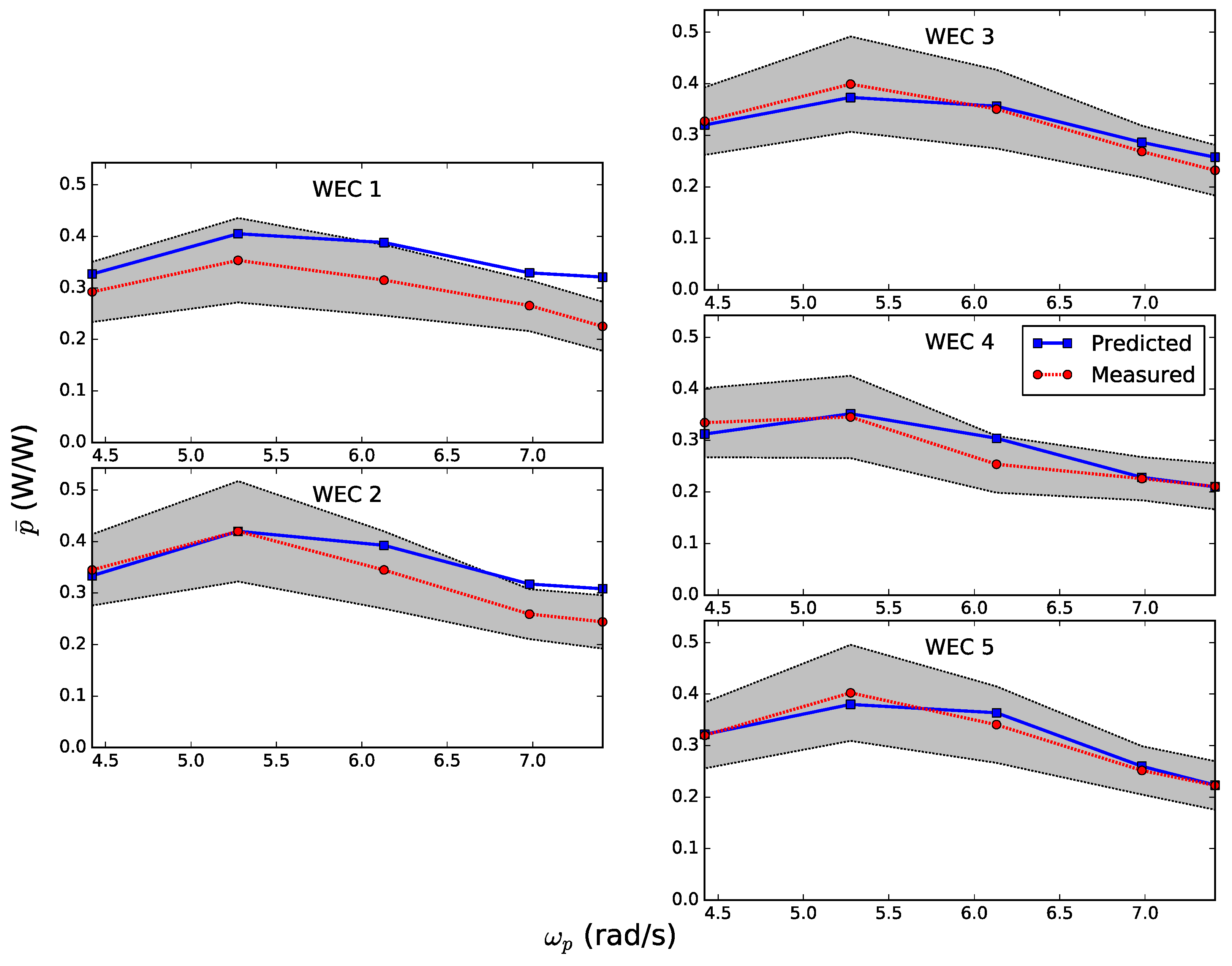
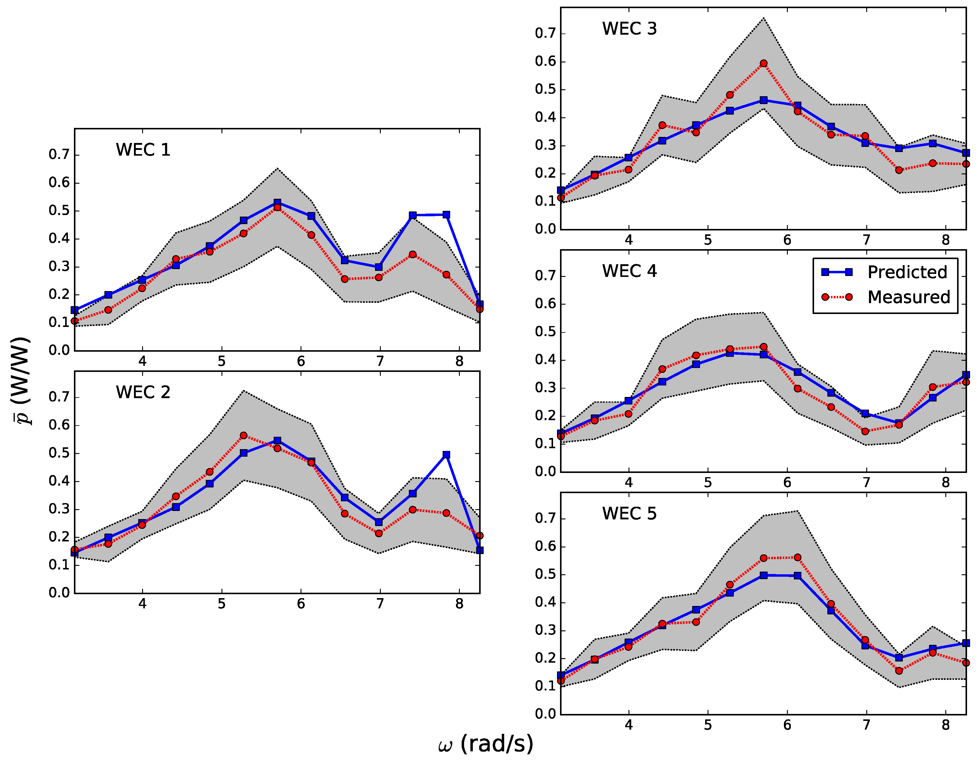
Figure 10 shows the predicted (blue line) and measured (red line) capture factor for the power absorption test and for each WEC when monochromatic waves are considered. The first is obtained through Equation (14) and the second through Equation (12).

Figure 10 shows that the predicted trend is in good agreement with the measured trend. With regard to the magnitude of the absorbed power, the predictions are observed to be significantly smaller than the measurements for both WECs 1 and 2 at the range of frequencies between 7 and 8 rad/s. However, the difference in magnitude seems to be partially covered by taking into account two standard deviations of the measured mean value (red dots).

It appears that resonance occurs at approximately 5.7 rad/s. At resonance, the uncertainty on the measured incident wave power (Section 6.1) is observed to be the largest. Therefore, the maximum deviation shown in Figure 10 for the measured data is associated to resonance, and corresponds to approximately $\pm$40% the mean value (red dots).

In contrast with the high accuracy observed for diffraction and radiation tests, the numerical model seems to be less accurate in the prediction of the power absorption in monochromatic waves. Nevertheless, the uncertainty on the generated waves is seen to cover the difference between the predictions and the measurements for most of the considered wave frequencies and for all the WECs.

Figure 11 shows the predicted (blue line) and measured (red line) capture factor for the power absorption test and for each WEC when panchromatic waves are considered. The first is obtained through Equation (20) and the second through Equation (17).

From Figure 11, the matching between predictions and measurements ends up improving when considering panchromatic waves. Hence, prediction errors appear to be attenuated by considering a spectrum with many wave frequencies. This is important since, as previously mentioned, panchromatic waves are a better approximation to real sea states than monochromatic waves. The maximum deviation shown in Figure 11 for the measured data corresponds to approximately $\pm$20% the mean value (red dots).

6.5. Prediction Errors

The MAPE for each of the tests and for each WEC is reported in

Table 3. MAPE (%) of the numerical model predictions for diffraction, radiation, and power absorption tests.

Test	WEC 1	WEC 2	WEC 3	WEC 4	WEC 5
Diffraction	23.30	8.84	7.42	5.93	8.67
Radiation	22.77	7.90	9.50	5.43	13.05
Power Absorption 1	23.16	16.75	15.85	13.54	12.03
Power Absorption 2	23.24	13.20	5.59	5.95	3.29

Notes: ¹ Monochromatic and ² panchromatic waves.

.

Table 3 shows that the predictions made for the WEC 1 lead to the highest MAPE. For the rest of the WECs, the MAPE is bounded by approximately 17%, i.e., the predictions are off by less than 17% on average. The smallest errors yield from the resultant moment predictions made for the WEC 4, which do not exceed 6% on average. Thus, it seems that the numerical model systematically provides poor estimates for the WEC 1 and better estimates for WEC 4 so that extreme errors appear to be associated with the positioning of the WECs in the array. This stands out the limitations in the physical model to effectively reproduce 2D long-crested plane waves propagating in only one direction.

The reflections due to the presence of the side-walls, the beach and, to a smaller extent, the paddles, led to undesired 3D wave effects, which were not accounted for in the numerical model. The undesired reflection effect was intended to be overcome by visually selecting a reduced time interval of the measurement record, as explained in Section 4, and by the analysis of panchromatic waves. Further analysis of the generated waves (Section 6.1) revealed this inconsistency and was then used to define a range of possible values for the measured amplitude moment and absorbed power shown as the grey region in Figure 8, Figure 9, Figure 10 and Figure 11. The predictions were then seen to fall within this region for most of the studied wave frequencies.

The uncertainty associated with the numerical model is hereafter studied through the distribution of the percentage error defined in Section 5.

Table 4. Mean value $\mu$ and standard deviation $\sigma$ of the percentage error $ϵ$ (%) for the prediction of resultant moments and power absorption.

	$\mathit{\mu }$ (%)	$\mathit{\sigma }$ (%)
Resultant moment (wave forces)	6.71	10.71
Power absorption	7.78	15.17

shows the mean value and the standard deviation of the percentage error for the prediction of resultant moments and power absorption.

It is readily apparent from Table 4 that the numerical model tends to predict larger values than the ones measured in the physical model by approximately 7%.

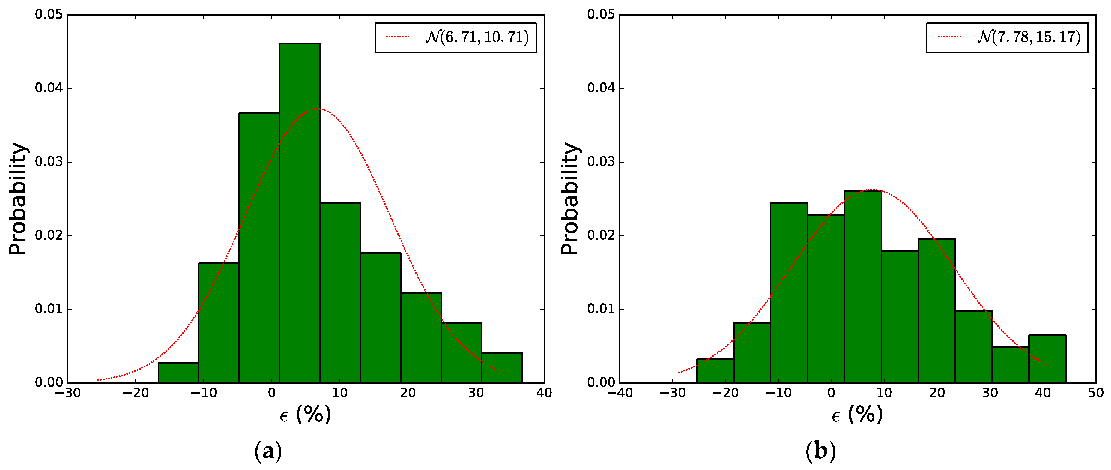
Figure 12 shows the percentage error histogram for the case of wave forces (a) and power absorption (b).

Figure 12 shows that it is safe to model the distribution of the percentage error as a normal with mean and standard deviation those reported in Table 4:

$${\widehat{M}}^T~\left(1+\frac{\mathcal{N}\left(6.71,10.71\right)}{100}\right)M^T,$$

(26)

for the prediction of wave forces; and:

$$\widehat{\overline{p}}~\left(1+\frac{\mathcal{N}\left(7.78,15.17\right)}{100}\right)\overline{p},$$

(27)

for the prediction of power absorption; with $~\mathcal{N}\left(\mu ,\sigma \right)$ denoting equal distribution of a normal with mean $\mu$ and standard deviation $\sigma$. Therefore, it is also safe to take the percentage errors $\pm$17.5% and $\pm$23.0% as the bounding errors for more than 68% of the predictions of wave forces and power absorption, respectively.

7. Conclusions

In order to validate the WEC array hydrodynamics tool presented in [16], a set of wave basin experimental tests for an array of five-point absorbers was conducted in the deep-water wave basin at Aalborg University. The WECs were equipped with advanced PTO simulators capable of accurately reproducing the effect of linear control strategies, thus improving the data quality obtained in [18] and [19]. The study then includes a comparison between experimental measurements and numerical predictions to estimate the uncertainty in the numerical model.

Diffraction tests where the WECs were fixed at their undisturbed mean position while excited by monochromatic waves and radiation tests where one of the WECs in the array was forced to move, while the rest were fixed, were used to assess the uncertainty in the prediction of wave forces. Overall, the results showed that the percentage error is less than $\pm$17.5%, on the safe side, for more than 68% of the predictions from a total of 130 predictions, with a positive average error of approximately 7%.

Power absorption tests where the WECs were operating under linear damping PTO systems in monochromatic and panchromatic waves were used to assess the uncertainty in the power absorption predictions. Overall, the results showed that the prediction error is less than $\pm$23.0%, on the safe side, for more than 68% of the predictions from a total of 90 predictions, with a positive average error of approximately 8%.