1. Introduction
With the accelerated pace of modern life, more and more perishable food is sold in marts or retail groceries. The increase in demand for perishable food brings about more profit, while the increased demand also makes it more difficult to manage with more quantities and varieties. Because of the short life of perishable food, all the items should be sold out before their “sell-by date”, or they have to be thrown away. Every year, the scale of spoilage is quite large in retail stores. According to Ferguson and Ketzenberg [
1], the attrition rate reaches as high as 15% during the time perishable food is sold in retail stores. At the same time, the gross profit of perishable food is relatively high because of its mass spoilage and the difficulty in managing it. Therefore, a highly efficient operation and rational design of the food retail chain may provide great potential to reduce spoilage and increase profit [
2,
3]. Since the quality of perishable food is decaying all the time and the consumption rate is affected by many factors, such as price, shelf space, discount rate, and so on, we should comprehensively consider all these important factors in designing the perishable food retail chain. In this paper, we determine the pricing and order strategy and shelf space allocation to maximize the food retailer’s profit.
The supply chain design for perishable products has attracted a great deal of attention in the industry recently. As the loss rate in retail stores is not quite satisfactory, a great number of models for managing perishable products have been developed. There are three main approaches to model the perishability of food. First, it is assumed that the perishable product has a fixed or random lifetime. For example, Zhou and Yang [
4] determined the optimal replenishment policy for items with a stock-dependent demand rate and a fixed lifetime. Second, perishability is defined as a proportion of the product disappearing or becoming outdated, while the value of the remainder does not change. Related work by Mandal and Phaujdar [
5], which presented an inventory model for deteriorating items, assumed that the demand rate is a linear function of the current stock level and the deterioration rate could be constant or time-dependent. Third, some models assume that the value of a perishable product deteriorates as over time. Zanoni and Zavanella [
6] considered the economic aspects and energy efforts together with the assumption that the quality of perishable food decays exponentially. As the third assumption is realistic in most perishable food cases, it is also applied in this research. Since the value of a perishable product decreases over time, the demand for the product also goes down. Hence, the pricing and discount strategy plays an important role in the sales promotion, especially when the product approaches its expiration date. Hong and Lee [
7] decided the price, lead time, and lateness penalty to maximize the total profit for a price- and time-sensitive market. Wang and Li [
8] developed a pricing model to maximize the total profit for perishable food supply chains.
Besides the perishable product’s quality and price, the shelf space allocated is also an important factor which may affect the consumption rate. Larger shelf space can attract more visibility and bring about more sales; further, larger shelf space may also imply the product is popular and in season. Lynch and Curhan [
9] assumed a quadratic relationship between the shelf space allocated to a product and the consumption rate in supermarkets. Wang and Gerchak [
10] developed a coordination mechanism where the manufacturer offers a holding cost subsidy to coordinate the channel when the retailer’s demand is shelf space–dependent. Mohsen et al. [
11] proposed an integrated vendor-buyer inventory model to maximize the channel profit, with the assumption that the buyer has a two-stage inventory, a warehouse and a display shelf, and the demand is dependent on the amount of items displayed. Since few papers have considered shelf space allocation and pricing strategies simultaneously in the management of the perishable food retail chain, this research deals with the problem and provides an efficient food retail chain design for food retailers.
2. Model Formulation for the Single-Item Food Retail Chain
In this section, we model the whole course of the perishable food sold in a retail store, from the arrival of the product, selling it on the shelf and discount rack, to the disposal of the expired goods. The following notations are used through the whole paper. Additional notations are introduced when required.
| q | quality of the perishable food |
| q(t) | quality of the perishable food at time t |
| q0 | initial quality of the perishable food |
| λ | deterioration rate of the perishable food |
| p | selling price of the perishable food |
| ng | shelf space allocated to the perishable food |
| a | parameter of market scale for the perishable food |
| b | parameter of price elasticity for the perishable food |
| c | parameter of demand sensitivity to shelf space allocated to the food |
| d | parameter of demand sensitivity to quality of the food |
| m | parameter of opportunity cost for the current shelf space allocation |
| θ | ratio of discount price to original price of the perishable food (1 − θ is the discount rate) |
| f | discount attraction rate of the perishable food |
| t0 | food’s sales time on shelf |
| T | shelf lifetime of the perishable food |
| D1(t) | demand of the perishable food sold on shelf without discount at time t |
| D2(t) | demand of the perishable food sold on discount rack at time t |
| D(t) | demand of the perishable food during its shelf life |
| Q | order quantity of the perishable food |
| C0 | purchasing cost per unit of the perishable food |
| α | no discount price for purchasing the perishable food |
| β | discount sensitivity to order quantity Q for purchasing the perishable food |
| π | total profit of the perishable food retail chain |
| L | shelf space capacity |
2.1. Quality Deterioration
Quality deterioration is a complex course for perishable food. Tracking and predicting the quality of perishable food was quite a difficult task before modern technologies were developed, such as radio frequency identification (RFID), wireless sensor technology and the humidity-temperature sensor. Nowadays, with these technologies and quality prediction models, we can predict the remaining shelf life of a perishable product as its quality, which is the main interest for retailers and customers [
12,
13,
14,
15]. According to Labuza [
12], the quality degradation of perishable food is affected by several factors: the storage time, the ambient temperature, and the ambient atmosphere condition. In more detail, the quality degradation can be expressed by the following equation:
In Equation (1),
n is the chemical order of the reaction. In this equation,
n can be equal 0 or 1, depending on the degradation course of the product. When
n = 0, the quality decays at a constant rate. When
n = 1, the quality decays exponentially, which is more realistic and hence used in this research.
k0 is a constant rate,
Ea is the activation energy, which is an empirical parameter reflecting the exponential temperature,
R is the gas constant, and
T0 is the absolute temperature. By solving Equation (1), the quality of a perishable product at time
t can be described as:
In a retail grocery store, the temperature and atmosphere condition are usually stable. Therefore, we introduce
λ as the deterioration rate to reduce the complexity. Let
, and hence the quality at time
t becomes:
2.2. Demand Model
In a mart or retail grocery store, the consumption rate of perishable food is affected by many elements, such as the arrival rate of customers, price, quality, discount rate, and so on. In this research, we assume the consumption rate depends on three factors at first:
p,
q(
t), and
ng. First, customers are assumed to be able to distinguish the quality of the food. Then, larger shelf space can attract more visibility and imply that the product is popular, as mentioned in the literature. Consequently, the demand function can be described as:
In Equation (4), as we allocate
ng shelves to the product, there is a corresponding cost for these shelves,
mng2 per unit time. The assumption has been used in Swami and Shah [
16].
While after a certain period, the quality of perishable food decreases and its shelf life is about to end, the consumption rate will therefore go down. In a mart or retail grocery, the perishable products near their shelf life are usually taken from the shelves and sold on a discount rack. In this case, the shelf space does not affect the product’s sale and the discount rack can attract much attention especially when the discount policy is stable and normalized. Therefore, we assume the demand function after discount is:
Then, the demand function over the shelf life time can be described as:
2.3. Modeling the Single-Item Food Retail Chain
In the above part, we have modeled the quality and demand of perishable food in a retail store. Now the total profit model for the whole food retail chain is developed. There are several elements in the retailer’s profit: the sales revenue, shelf space cost, purchasing cost, and disposal cost.
First, we calculate the profit earned when the product is sold on the shelves by:
Second, since ng shelves are allocated to the product from the beginning to t0, the corresponding cost is t0mng2.
Third, the profit earned during the time the product is sold on the discount rack (this profit may be negative) is:
Fourth, let Q and C0 denote the order quantity and the purchasing cost per unit, respectively. For small retailers, C0 is usually a constant. For big retailers, the supplier may offer a wholesale discount to promote the product. Here, we assume the supplier offers a continuous discount function C0 = α − βQ, where α is the no-discount price and β is the discount sensitivity to Q. Then, the total purchasing cost is C0Q = (α − βQ)Q.
Finally, all the perishable products may not be sold out by the end of their shelf life. The remainder needs disposing, which may cause carbon emissions, environmental pollution, and corresponding cost. Let
Cd denote the disposal cost per unit. Then, the total disposal cost is:
Consequently, the total profit of the food retail chain is:
In Equation (10), p, ng and Q are determined to maximize the total profit. The other parameters are assumed to be given.
3. Optimal Solution for the Single-Item Food Retail Chain
In this section, we prove there is an optimal solution to maximize the total profit. First, we can see that
π is a polynomial of
Q once
p and
ng are given. Taking the first and second derivative of
π with respect to
Q, we get:
From
, we can obtain
. Since the only constraint is
, if
, then
. It is obvious that the parameter values are not reasonable. The value of
β may be too large. Therefore,
. For
π decreasing on [0, (
α +
Cd)/2
β],
is the optimal solution, which means all the products should be sold by the end of their shelf life. Therefore, there is no disposal cost. Substituting
into
π, the total profit becomes:
The Hessian matrix of
π is:
From Equations (15)–(17), we can see that , , and are all constants. Since β is quite small, and are usually less than 0. In this situation, if H > 0, the optimal point obtained from is the maximum point; if H < 0, is a saddle point, then the maximum point is at the boundary. Obviously, it is not realistic in practice; if H = 0, it cannot be judged what the point is. This situation is almost impossible because , , and are all constants. When (or ), which means when p (or ng) tends to infinity, the profit is infinity; this result is obviously not realistic. In this situation, the parameter values are not reasonable.
4. The Multi-Item Food Retail Chain
In this section, we extend the single-item retail chain model into a multi-item one. The following assumptions are needed to simplify the problem. First, the consumption of each item is assumed to be independent from that of the others. Second, the capacity of the shelf space is limited. Third, since the deterioration rate and replenishment cycle of each item are different from those of the others, all the items are replenished separately. Fourth, the objective of the multi-item retail chain is to maximize the summation of each item’s profit per unit time rather than the total profit per unit cycle, because the replenishment cycle of each item is different. Let superscript
i denote the index of each item and
L denote the shelf space capacity. Therefore, the objective function of the multi-item retail chain is:
The shelf space cost in the above objective function is useful when we determine each item’s shelf space. However, when the total profit per unit time is calculated, the retailer does not take the shelf space cost into account. The shelf space is considered as a limited resource. Therefore, the total profit per unit time without the shelf space cost is:
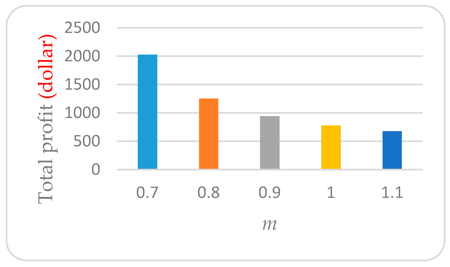
The summation of each item’s shelf space may be larger or smaller than the shelf space capacity when the opportunity cost of the shelf space (m) is given. From the objective function we can see that each item’s shelf space allocated and the total profit per unit time are negatively correlated with the shelf space opportunity cost, so we could adjust the value of m to make the summation of each item’s shelf space equal to the shelf space capacity.
In the multi-item retail chain, the objective is to maximize the total profit per unit time with the shelf space cost. Since the replenishment cycle of each item is constant, the optimal solution obtained in
Section 3 will not change when the value of
m is given. Ji et al. [
17] developed a mathematical model for a multi-commodity, two-stage transportation and inventory problem, which was solved by CPLEX Optimizer. CPLEX Optimizer is a high-performance mathematical programming solver for linear programming, mixed integer programming and quadratic programming. In this part, we develop a simple algorithm to find the optimal solution for the multi-item retail chain.
Algorithm
Step 1: Input all the values of the parameters and find the upper and lower bound of m.
Step 2: Let mk (k = 1, 2 …, 10) be equally distributed between the upper and lower bound. Set an acceptable error e. Calculate each item’s , pi, Qi and πi with each mk and П.
Step 3: If there is an mk that makes , the current result is the optimal solution. Otherwise, the mk that makes and the mk+1 that makes become the new upper and lower bound of m. Go to Step 2.
5. Numerical Experiments and Real-Life Examples
In this section, we first evaluate the effects of some key parameters and then use some real-life data from physical retail stores to validate the model.
5.1. Parameters Evaluation
We input different values of the key parameters, the discount rate and the opportunity cost of shelf space, and show the effects on the total profit and optimal solutions in the single-item retail chain.
Table 1 shows the values of the input parameters.
Since the values of the parameters are given, we can calculate the value of the Hessian matrix, where H = 147.20 > 0. (p*, ng*) is the maximum point. In the model, we assume that the discount rate 1 − θ is a constant, while it is also an important decision variable in the retail store. Therefore, we attempt to find an approximation of the optimal discount rate by numerical analysis.
Table 2 shows that as the discount rate (1 −
θ) decreases, the shelf space allocated, price, and order quantity also decrease. That is because the decrease in the discount rate reduces the demand on the discount rack. The retailer has to lower the price to promote the market, and hence lower the shelf space to save some shelf space cost. From
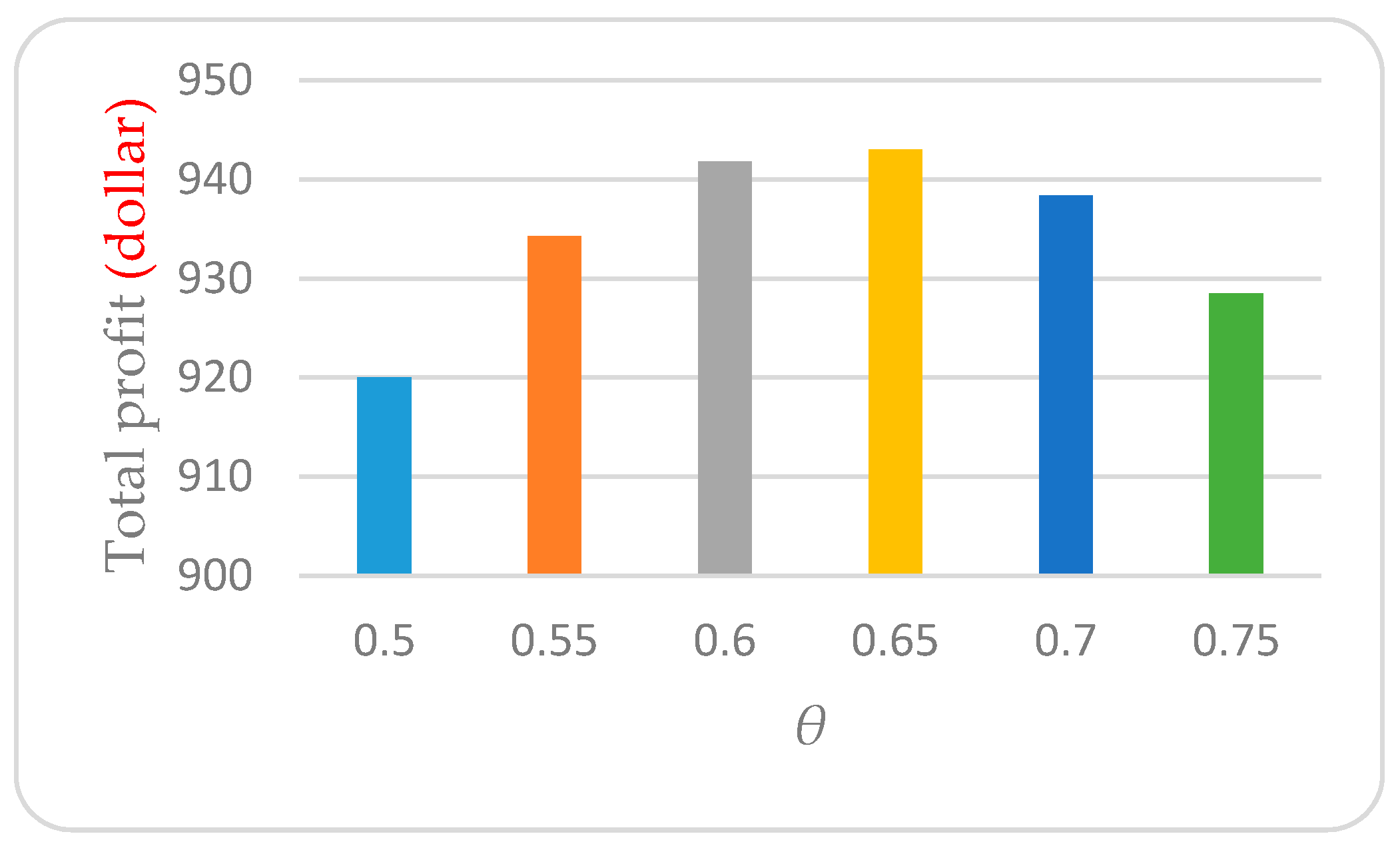
Figure 1, we can see that the total profit seems concave in
θ and reaches its maximum around
θ = 0.65, while in the reality,
θ is usually correlated with the discount rack attraction rate, which needs further research in the retail store to investigate their relationship.
The opportunity cost of the shelf space is also an important parameter which may affect the space allocation and total profit significantly.
Table 3 and
Figure 2 show the effects of
m on the total profit and decision variables.
Table 3 and
Figure 2 show that the total profit and all the variables decrease when
m goes up. That’s due to the fact that as the opportunity cost of the shelf space increases, the retailer reduces the shelf space and lowers the price to improve the utilization rate of the shelves. That can explain why the product on the shelves with the best position in a mart always changes. Usually, the best or largest shelves are only allocated to the product in season or on discount.
In the second case, we show the effects of the shelf space capacity on the total profit per unit time in the multi-item retail chain. It is assumed that there are five items in the retail chain.
Table 4 shows the value of the input parameters.
In the multi-item retail chain, the shelf space capacity is the main constraint which is a fundamental resource for the retailer. Usually, customers are willing to go to large marts, which can provide comfortable shopping conditions, a variety of goods, and low prices.
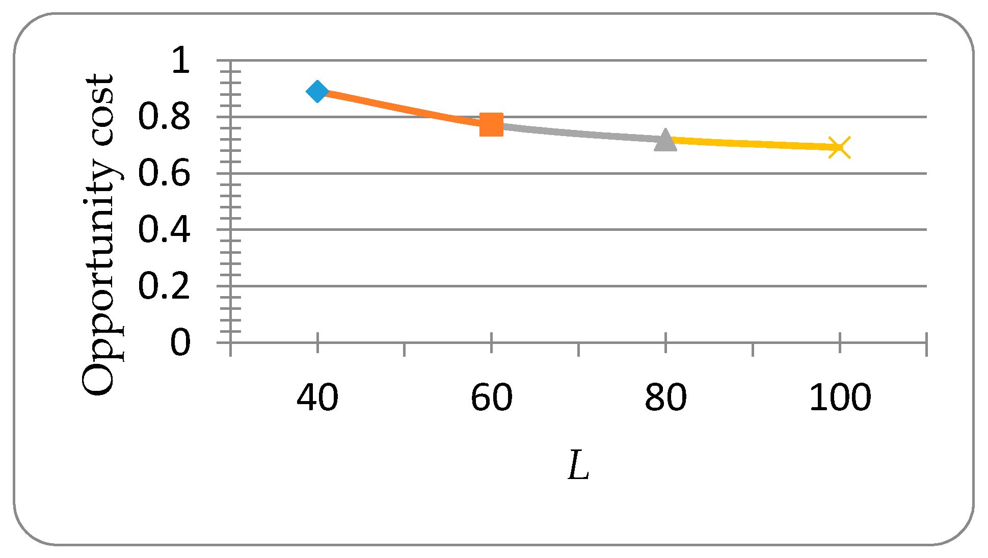
From
Figure 3, we can find that larger shelf space could reduce the opportunity cost of the shelf space.
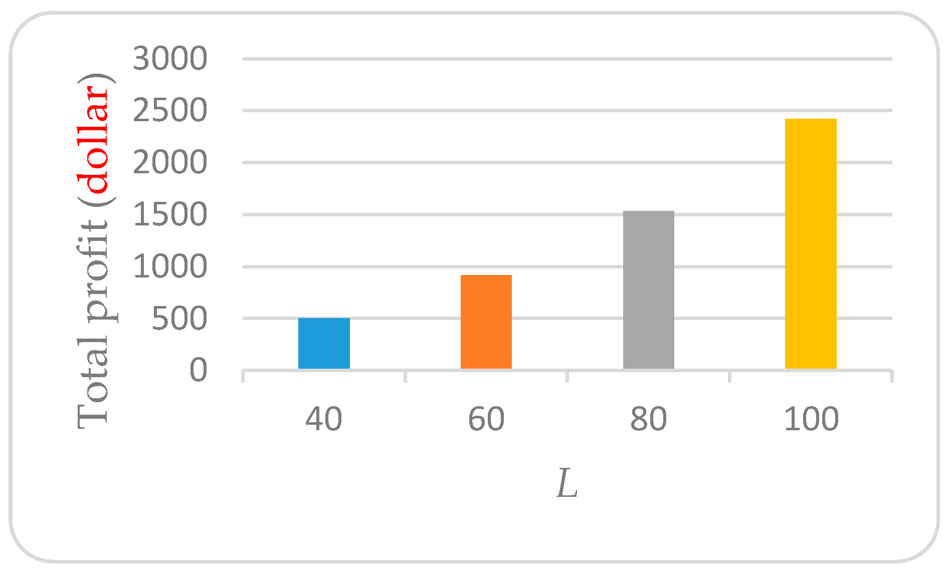
Figure 4 shows that the total profit grows as the shelf space capacity increases. In reality, besides the increase of the shelf space capacity, the retailers also try to expand the types of goods, which may attract more customers and sales to increase the total profit rapidly.
5.2. Real-Life Examples
In this part, we use some real-life data to show the model’s application in a practical case. The data we use are obtained from physical retail stores, which have been applied in Wang and Li [
8] and Desmet and Renaudin [
18]. To satisfy the assumptions well in
Section 4, two kinds of perishable products are considered in the case, meat and vegetables. Meat and vegetables are the two kinds of most common perishable foods in the market, and they are quite representative in real life. Additionally, empirical data can be obtained easily from published reference paper. The common parameters of a meat product sold in different stores are shown in
Table 5.
Table 6 shows the different parameters and results. Then, we consider a vegetable product in different stores. The parameters and results are shown in
Table 7 and
Table 8. Due to the fact that there is no prior empirical data of the effect of product quality on the consumption rate, we assumed that the effect of quality equals the price sensitivity, as Wang and Li [
8] did.
From
Table 5 and
Table 7 we can see that the deterioration rate of the meat product is 0.0067 per hour and the vegetable product’s deterioration is 0.0216 per hour. Since the vegetable perishes much more quickly than the meat, the vegetable’s replenishment cycle is shorter than the meat’s. From Desmet and Renaudin [
18], we get that the consumption rate of meat products is not quite sensitive to the shelf space allocated (around 0.35) and that of the vegetable is relatively sensitive to the shelf space allocated (around 0.57). Furthermore, the shelves for meat products contain a refrigerating system, which reduces the meat’s deterioration rate but makes the shelf space for meat quite expensive. Therefore, the retailer prefers to allocate smaller shelf space to each meat product than the vegetable product.
As there is little empirical data on perishable products, we assume the meat product in different stores as different products in a retail store and validate the multi-item retail chain model. The input parameters are shown in
Table 5. The results for the multi-item retail chain are shown in
Table 9.
From
Table 9 we can see that each item’s price goes up as the shelf space capacity increases. That is because larger shelf space decreases the opportunity cost of the shelf space, and larger shelf space attracts more sales, which could offset the effect of the increased price. This may not conform to the actual situation. The reason is that as the shelf space capacity increases, more customers are attracted and hence the market scale is expanded. In our case, the market scale remains the same. Another reason is that as the shelf space capacity increases, the retailer usually adds more varieties of items. When one item is added, the total profit per unit time will increase. If not, the retailer will not choose to add the item. The increased profit means the opportunity cost of the shelf space goes up, and the retailer will decrease the price to improve the utilization rate of the shelves. However, the total profit may not always increase with the number of items, for too much variety of items may increase the operation cost and also dazzle customers. Meanwhile, the items on a shelf may be replenished too frequently with small shelf space, which may increase the labor cost.
6. Conclusions
This research attempts to improve the retail chain design for perishable food in a retail store by comprehensively evaluating the pricing strategy, shelf space allocation, and replenishment policy with the help of modern tracking technologies. This paper may have great potential in spoilage reduction and profit improvement for the food retail chain management. First, we developed a mathematical model for perishable food with a single item. The results showed that the discount rate is positively related to the decision variables (price, shelf space, and order quantity) and its optimal value can be obtained by numerical analysis. Larger shelf space could reduce the opportunity cost of the shelf space and bring about more profit. The results also showed that the discount and pricing strategy and shelf space can greatly affect the performance of the retail chain, so the design of the food retail chain should evaluate all the relevant parameters carefully. Then, the single-item retail chain was extended into a multi-item one with a shelf space capacity. As shown in the results, when larger shelf space is available, the retailer should allocate more space to the products whose demands are sensitive to the shelf space and expand the types of goods, which may attract more customers and sales.
Acknowledgments
The authors are grateful to the editors and anonymous reviewers for providing the valuable comments. The research was supported by the National Natural Science Foundation of China (Grant No. 71501090), the Natural Science Foundation of Jiangsu Higher Education Institutions of China (Grant No. 14KJD410001) and the Jiangsu Philosophical-social Science Program (2016SJB630113).
Author Contributions
Yujie Xiao conceived and designed the experiments; Shuai Yang performed the experiments; Yujie Xiao and Shuai Yang analyzed the data; Yujie Xiao contributed analysis tools; Yujie Xiao and Shuai Yang wrote the paper.
Conflicts of Interest
The authors declare no conflict of interest. The founding sponsors had no role in the design of the study; in the collection, analyses, or interpretation of data; in the writing of the manuscript, and in the decision to publish the results.
References
- Ferguson, M.E.; Ketzenberg, M.E. Information Sharing to Improve Retail Product Freshness of Perishables. Prod. Oper. Manag. 2006, 15, 57–73. [Google Scholar]
- Mouron, P.; Willersinn, C.; Möbius, S.; Lansche, J. Environmental Profile of the Swiss Supply Chain for French Fries: Effects of Food Loss Reduction, Loss Treatments and Process Modifications. Sustainability 2016, 8, 1214–1223. [Google Scholar] [CrossRef]
- Aiello, G.; la Scalia, G.; Micale, R. Simulation analysis of cold chain performance based on time–temperature data. Prod. Plan. Control 2012, 23, 468–476. [Google Scholar] [CrossRef]
- Zhou, Y.W.; Yang, S.L. An Optimal Replenishment Policy for Items with Inventory-level-dependent Demand and Fixed Lifetime under the LIFO Policy. J. Oper. Res. Soc. 2003, 54, 585–593. [Google Scholar] [CrossRef]
- Mandal, B.N.; Phaujdar, S. An Inventory Model for Deteriorating Items and Stock-dependent Consumption Rate. J. Oper. Res. Soc. 1989, 40, 483–488. [Google Scholar] [CrossRef]
- Zanoni, S.; Zavanella, L. Chilled or Frozen? Decision Strategies for Sustainable Food Supply Chains. Int. J. Prod. Econ. 2012, 140, 731–736. [Google Scholar] [CrossRef]
- Hong, K.S.; Lee, C. Optimal Pricing and Guaranteed Lead Time with Lateness Penalties. Int. J. Ind. Eng. Theory 2013, 20, 153–162. [Google Scholar]
- Wang, X.; Li, D. A Dynamic Product Quality Evaluation Based Pricing Model for Perishable Food Supply Chains. Omega 2012, 40, 906–917. [Google Scholar] [CrossRef]
- Lynch, M.; Curhan, R.C. A Comment on Curhan’s “The Relationship between Shelf Space and Unit Sales in Supermarkets”. J. Mark. 1974, 11, 218–220. [Google Scholar] [CrossRef]
- Wang, Y.; Gerchak, Y. Supply Chain Coordination When Demand is Shelf-space Dependent. Manuf. Serv. Oper. 2001, 3, 82–87. [Google Scholar] [CrossRef]
- Mohsen, S.S.; Anders, T.; Mohammad, R.A.J. An Integrated Vendor–buyer Model with Stock-dependent Demand. Transport. Res. E-Log. 2010, 46, 963–974. [Google Scholar]
- Labuza, T.P. Application of Chemical-kinetics to Deterioration of Foods. J. Chem. Educ. 1984, 61, 348–358. [Google Scholar] [CrossRef]
- Hertog, M.L.; Uysal, I.; McCarthy, U.; Verlinden, B.M.; Nicolaï, B.M. Shelf Life Modelling for First-expired-first-out Warehouse Management. Philos. Trans. R. Soc. A Math. Phys. Eng. Sci. 2014, 372, 1–15. [Google Scholar] [CrossRef] [PubMed]
- Sciortino, R.; Micale, R.; Enea, M.; la Scalia, G. A WebGIS-based System for Real Time Shelf Life Prediction. Comput. Electr. Agric. 2016, 127, 451–459. [Google Scholar] [CrossRef]
- La Scalia, G.; Settanni, L.; Corona, O.; Nasca, A.; Micale, R. An Innovative Shelf Life Model based on Smart Logistic Unit for an Efficient Management of the Perishable Food Supply Chain. J. Food Process Eng. 2015. [Google Scholar] [CrossRef]
- Swami, S.; Shah, J. Channel Coordination in Green Supply Chain Management: The Case of Package Size and Shelf-space Allocation. Technol. Oper. Manag. 2011, 2, 50–59. [Google Scholar] [CrossRef]
- Ji, P.; Chen, K.J.; Yan, Q.P. A Mathematical Model for a Multi-Commodity, Two-Stage Transportation and Inventory Problem. Int. J. Ind. Eng. Theory 2008, 15, 278–285. [Google Scholar]
- Desmet, P.; Renaudin, V. Estimation of Product Category Sales Responsiveness to Allocated Shelf Space. Int. J. Res. Mark. 1998, 15, 443–457. [Google Scholar] [CrossRef]
© 2016 by the authors; licensee MDPI, Basel, Switzerland. This article is an open access article distributed under the terms and conditions of the Creative Commons Attribution (CC-BY) license (http://creativecommons.org/licenses/by/4.0/).


