Marginal Abatement Cost of CO₂ in China Based on Directional Distance Function: An Industry Perspective

Abstract

Industrial sectors account for around 70% of the total energy-related CO₂ emissions in China. It is of great importance to measure the potential for CO₂ emissions reduction and calculate the carbon price in industrial sectors covered in the Emissions Trading Scheme and carbon tax. This paper employs the directional distance function to calculate the marginal abatement costs of CO₂ emissions during 2005–2011 and makes a comparative analysis between our study and the relevant literature. Our empirical results show that the marginal abatement costs vary greatly from industry to industry: high marginal abatement costs occur in industries with low carbon intensity, and vice versa. In the application of the marginal abatement cost, the abatement distribution scheme with minimum cost is established under different abatement targets. The conclusions of abatement distribution scheme indicate that those heavy industries with low MACs and high carbon intensity should take more responsibility for emissions reduction and vice versa. Finally, the policy implications for marginal abatement cost are provided.

1. Introduction

Following several reports issued by the IPCC (Intergovernmental Panel on Climate Change), which have pointed out that climate change is closely related to human activities [1,2], mounting pressure from the international community has called for a series of efforts in reducing global carbon dioxide emissions in order to alleviate the greenhouse effect [3]. In 2006, China became the largest carbon emitter, surpassing the United States for the first time and encountering more pressure from other countries. The Chinese government has promulgated an emissions reduction target that requires carbon intensity (CO₂ emissions per unit of gross domestic product) to be reduced by 40%–45% by 2020, with 2005 as the reference year.

In the context of pursuing climate policy targets, China has made a great effort to mitigate its rising trend of CO₂ emissions [4]. There are two main types of emissions reduction policies based on market mechanisms: carbon tax policy and Emissions Trading Scheme (ETS) [5]. The former is characterized by price control [6], and the latter is characterized by total amount control [7], both of which can influence the market by use of price leverage [8]. Against this backdrop, the Chinese government drew on foreign experience and gradually carried out the ETS and carbon tax. This raises two questions. (1) How can the maximum social benefit be reaped? Lots of previous studies proposed that an optimal tax rate should be equal to the marginal abatement cost (MAC) of CO₂. A low-level tax rate cannot stimulate emissions reduction, and a high tax rate can cause erosion of industries’ competitiveness [9]; (2) How can mandatory emissions reduction targets be reached in an effective way? The market price of an ETS and the MAC of CO₂ are certainly the information every enterprise needs [10]. The enterprises will screen a list of policy options to devise the best abatement strategies, such as cutting carbon emissions, buying emissions allowances, selling emissions allowances, and so on, all of which depend on the comparison between the MAC and the price of the emissions allowance.

Marginal abatement cost has recently become a standard policy tool in assessing climate change mitigation schemes [11,12]. Estimating the MAC of CO₂ in some industrial sectors in China can provide valuable information for enterprises to optimize the carbon abatement strategies [13]. Furthermore, a clear perspective of the MAC in each industry can also help the government to set an optimal carbon tax rate.

We try to use the environmental directional distance function to estimate the CO₂ marginal abatement cost in some industrial sectors. Then, we also discuss the practical application of marginal abatement cost, including the estimation of a marginal abatement cost curve and the establishment of an abatement distribution scheme. Finally, based on the conclusions in this paper, we put forward some policy recommendations. In brief, the results and analyses in this paper can provide policy recommendations for the Chinese government to shape an optimal emissions reduction policy. The rest of the paper is organized as follows: Section 2 presents the literature review. Section 3 provides a model description. Section 4 shows the results and analyses, and Section 5 discusses the conclusions and policy implications.

2. Literature Review

Facing international pressure to reduce GHG emissions, more and more scholars have begun to study emissions reduction costs at home and abroad. Unfortunately, though, knowledge about carbon pricing is still limited in China.

Marginal abatement cost refers to the costs associated with eliminating an additional unit of undesirable output. According to previous studies, the estimation methods of marginal abatement cost and the marginal abatement cost curve can be separated into several categories, such as a computable general equilibrium (CGE) model [14], a dynamic optimization approach [15], a hybrid model [16], and so on [17,18]. Among them, the distance function stands out due to its accuracy and modest data requirement. The distance function was first proposed for the analysis of shadow prices by Färe et al. [19,20,21,22], which can be regarded as an analytical framework consisting of a sequence of models. Classified by different estimation methods, two estimation methods, namely parametric and nonparametric ones, have been widely applied to estimate distance function [23].

As its name implies, the parametric method needs a pre-defined specific functional form. The translog form and the quadratic form are the two main forms used in estimating the parameters. We can divide the parametric method into two categories. The first category is Shephard distance functions, including Shephard input and output distance functions. Islas and Grande [24] calculated the MAC of SO₂ from 51 coal-fired power plants in the United States. Lee and Zhang [25] calculated the MAC of CO₂ in 30 Chinese manufacturing industries, and the results showed that the average price is $3.13/ton. Both of them used translog Shephard input distance functions. Moreover, the translog Shephard output distance functions are also applied by many scholars. Lee [26] calculated the MAC of CO₂ from 52 fossil-fueled electric power generators in South Korea. Ke et al. [27] divided China into eastern, central, and western areas and estimated the MAC of SO₂ in the three areas. The second category of the parametric method is directional distance functions. Translog function form is always used in Shephard functions, but it is unsuitable for the directional distance function due to the low performance of transfer property [28]. However, quadratic function can perfectly match the characteristics of directional distance function [29]. Zhou et al. [30] applied the quadratic directional distance function (DDF) approach to estimate the shadow price in several industrial sectors in Shanghai. Molinos et al. [31] estimated the MAC of CO₂ for wastewater treatment plants. Duan et al. [32] evaluated the energy and CO₂ emissions performance of China’s thermal power industry.

Another estimation method is the non-parametric method. It is widely acknowledged that data envelopment analysis (DEA), which was developed by Charnes and Cooper, is a popular non-parametric technique for parameter estimation [33]. With the deepening of the research and the increasing focus on the undesirable outputs, the DEA theory was banded together with the distance functions to solve energy, efficiency, and marginal cost issues. The first pioneer was Turner [34], who employed a sub-vector Shephard output distance function and a DEA model to estimate the abatement cost of several pollutants. From then on, the non-parametric method was widely accepted. Leleu [35] introduced a hybrid DEA model to solve a set of methodological debates in nonparametric shadow-pricing approaches. Mekaroonreung and Johnson [36] estimated a technical change effect on MAC of U.S. coal power plants. Chang and Hu [37] introduced a total-factor energy productivity change index to evaluate the energy productivity change of regions in China with a total-factor framework.

Note that, although there are lots of studies on MAC of CO₂ in China, most of them focused on the provincial level. Zhang et al. [38] estimated MAC of carbon emissions at the provincial level in China using both Shephard and directional distance functions. Wang et al. [39] calculated the MAC of CO₂ in 28 provinces using the nonparametric method. In addition, some related studies on other emissions were carried out by some scholars. Kaneko et al. [40] calculated the MAC of SO₂ in thermal power sector and explored empirical evidence for two hypotheses through a macro productivity analysis. Yuan and Cheng [41] calculated the MAC of SO₂, waste water, and soot using the data for 284 industrial sectors. In summary, the above literature provides a comprehensive discussion of the marginal abatement costs, but there are still some limitations in previous studies. There is a lack of research estimating the MAC of CO₂ in China’s industries. Meanwhile, further discussion of the applications of MAC is also scanty. On this basis, we have made an effort to estimate the marginal abatement cost of CO₂ at the industrial level, and explore the practical applications of marginal abatement cost.

3. Model Description

3.1. Sectors and Data

Selecting the evaluation object, as the first step of model analysis, is of great importance. Considering the “Classification and Code Standard of National Economy Industry” in China (GB/T4754-2011), we disaggregated the whole economy into two categories (light and heavy industry). Among them, the light industry and heavy industry are further disaggregated. The heavy industry is divided into 19 typical industrial sectors and the light industry is correspondingly divided into 20 typical industrial sectors. Finally, by merging and unifying the category of national production activities, a total of 39 sectors are obtained. For convenience, we marked the sectors as SEC 01, SEC 02, SEC 03, etc. The sectors and their corresponding codes are shown in

Table 1. Names and codes of 39 sub-sectors.

Sectors	Code	Sectors	Code
Mining and Washing of Coal	SEC 01	Manufacture of Foods	SEC 21
Extraction of Petroleum and Natural Gas	SEC 02	Manufacture of Beverages	SEC 22
Mining and Processing of Ferrous Metal Ores	SEC 03	Manufacture of Tobacco	SEC 23
Mining and Processing of Non-Ferrous Metal Ores	SEC 04	Manufacture of Textile	SEC 24
Mining and Processing of Nonmetal Ores	SEC 05	Manufacture of Textile Wearing Apparel, Footwear, and Caps	SEC 25
Mining of Other Ores	SEC 06	Manufacture of Leather, Fur, Feather and Related Products	SEC 26
Processing of Petroleum, Coking, Processing of Nuclear Fuel	SEC 07	Processing of Timber, Manufacture of Wood, Bamboo, Rattan, Palm, and Straw Products	SEC 27
Manufacture of Raw Chemical Materials and Chemical Products	SEC 08	Manufacture of Furniture	SEC 28
Manufacture of Non-metallic Mineral Products	SEC 09	Manufacture of Paper and Paper Products	SEC 29
Smelting and Pressing of Ferrous Metals	SEC 10	Printing, Reproduction of Recording Media	SEC 30
Smelting and Pressing of Non-ferrous Metals	SEC 11	Manufacture of Articles For Culture, Education and Sport Activity	SEC 31
Manufacture of Metal Products	SEC 12	Manufacture of Medicines	SEC 32
Manufacture of General Purpose Machinery	SEC 13	Manufacture of Chemical Fibers	SEC 33
Manufacture of Special Purpose Machinery	SEC 14	Manufacture of Rubber	SEC 34
Manufacture of Transport Equipment	SEC 15	Manufacture of Plastics	SEC 35
Manufacture of Electrical Machinery and Equipment	SEC 16	Manufacture of Communication Equipment, Computers and Other Electronic Equipment	SEC 36
Production and Distribution of Electric Power and Heat Power	SEC 17	Manufacture of Measuring Instruments and Machinery for Cultural Activity and Office Work	SEC 37
Production and Distribution of Gas	SEC 18	Manufacture of Artwork and Other Manufacturing	SEC 38
Production and Distribution of Water	SEC 19
Processing of Food from Agricultural Products	SEC 20	Recycling and Disposal of Waste	SEC 39

.

After finishing the selection and classification of sectors, we explain the data collection here to provide a clearer model setting. In order to estimate the industrial MAC of CO₂, we selected five variables that can be classified into three kinds. The desirable output is industrial output value, the undesirable output is CO₂ emissions, and the inputs contain labor, capital, and energy. The variables are shown in

Table 2. Data collection and specification.

Category	Indicator	Unit	Data Collection
Desirable output	Industrial output	108 China Yuan (CNY)	China Statistical Yearbook, China Industrial Economic Statistical Yearbook
Undesirable output	CO2 emissions a	104 ton	China Energy Statistical Yearbook, Guidelines for National Greenhouse Gas Inventories (IPCC)
Input	Labor input	104 People	China Industrial Economic Statistical Yearbook
	Capital input	108 CNY	China Industrial Economic Statistical Yearbook
	Energy input b	104 tons of coal equivalents (tce)	China Energy Statistical Yearbook, China Statistical Yearbook

^a CO₂ emissions is unavailable from any of the statistical yearbook; this data is calculated by the author himself; ^b All the energy input are converted into tce (tons of coal equivalents).

.

However, the data for CO₂ emissions are not directly available from any of the statistical yearbook. Following the previous studies [38], we calculated CO₂ emissions using Equation (1):

$$C{O}_2={\displaystyle \sum _{j=1}^n{a}_j\cdot C_j\cdot E_j\cdot CO{E}_j},$$

(1)

where j (j = 1, 2, …, 6) represents different types of fossil fuels. In order to avoid any repeated calculation, three kinds of traditional fossil fuels are taken into consideration. In addition, crude oil is further divided into gasoline, kerosene, diesel, and fuel oil. In Equation (1), a_j is the loss coefficient, C_j is the consumption of fossil fuels, E_j is the standard coal conversion factor, and COE_j is the emissions coefficient. Conversion factors and emissions coefficients are shown in

Table 3. Conversion factors and emissions coefficients of fossil fuels.

Energy	Loss Coefficient	Conversion Factor	Emissions Coefficient
Coal	3.2%	0.7143 tce/ton	2.7716 tCO2/tce
Gasoline	3.1%	1.4714 tce/ton	2.0306 tCO2/tce
Kerosene	3.7%	1.4714 tce/ton	2.1058 tCO2/tce
Diesel	3.6%	1.4571 tce/ton	2.1699 tCO2/tce
Fuel Oil	3.6%	1.4286 tce/ton	2.2667 tCO2/tce
Natural gas	2.1%	1.33 kgce/m3	1.6438 tCO2/tce

.

3.2. Directional Distance Function

First, we marked 39 industries as i (i = 1, 2, …, 39). The desirable industrial output values are marked as vector y and the CO₂ emissions are marked as vector b. In addition, capital input, labor input, and energy input are marked as vector k, l, and e, respectively. Then, input vector $x=(k,l,e)$ is introduced here. The joint production process can be modeled by a production technology that can be represented by an output possibility set $P(x)=\{(y,b):xcanproduce(y,b)\}$. The directional distance function is depicted in Figure 1.

In the directional distance function, a production unit E(b,y) is in the internal area of output possibility set. “Abate Emissions” is a typical CO₂ reduction path based on the selected direction vector. The direction vector $d=(d_y,-d_b)$ is a typical reduction strategy direction vector, which requires a proportional increase of industrial output value and a decrease in CO₂ emissions. The unit E moves along the direction vector EE’ to point E’, whose coordinate is $(b-{\beta }_1*d_b,y+{\beta }_1*d_y)$. Compared to E, the desirable output increased by ${\beta }_1*d_b$ and the CO₂ decreased by ${\beta }_1*d_y$. Moreover, there is another path named “Fixed Emission”. The unit E moves along the direction vector EE” to point E”. Given the same input, the CO₂ emissions are fixed while the desirable output is expanded. After comparing these two scenarios, we can notice that the emissions reduction strategy requires enterprises to sacrifice their immediate profits. Thus, the ratio of $\Delta y$ and $\Delta b$ can tell us the cost of emissions reduction.

Formally, the directional distance function is defined in Equation (2). There are three reasons to select g = (1, −1) as the direction vector. First and foremost, it means that the expansion of the desirable output is accompanied by the shrinkage of the undesirable output under a given level of inputs. Another reason is that this vector can help us simplify the process of estimating the unknown parameters and reduce the parameters to be estimated. Moreover, it also can meet with the transfer property of the directional distance function.

$${\overrightarrow{D}}_0(x,y,b;g_y,-g_b)=\max \{\beta :(y+\beta g_y,b-\beta g_b)\in P(x)\}$$

(2)

Based on former studies and the transfer property [11,30], we selected a quadratic function form to parameterize the directional distance function. Quadratic function of output directional distance function is depicted in Equation (3):

$$\begin{array}{c}{\overrightarrow{D}}_0(x_i,y_i,b_i;1,-1)=\alpha +{\displaystyle \sum _{n=1}^3{\beta }_n{x}_{ni}+\gamma y_i+\eta b_i+\frac{1}{2}{\displaystyle \sum _{n=1}^3{\displaystyle \sum _{n\prime =1}^3{\alpha }_{n,n\prime }{x}_{ni}{x}_{n\prime i}+\frac{1}{2}\lambda y_i^2+}}}\frac{1}{2}\theta b_i^2\\ +{\displaystyle \sum _{n=1}^3{\delta }_n{x}_{ni}{y}_i}+{\displaystyle \sum _{n=1}^3{\omega }_n{x}_{ni}{b}_i}+\phi y_i{b}_i\end{array}.$$

(3)

After determining the specific form of directional distance function, the estimation of the parameters in the function is a key step. Many studies put forward that minimizing all the deviation between decision-making units (DMUs) and efficient production frontiers can help us estimate all parameters [11]. Following the trace of previous studies, a target programming model is established. The statement is shown in the following equations:

$$\min {\displaystyle \sum _{i=1}^{39}[{\overrightarrow{D}}_0(x_i,y_i,b_i;1,-1)}-0]$$

(4)

$$\mathrm{s}.\mathrm{t}.{\overrightarrow{D}}_0(x_i,y_i,b_i;1,-1)\ge 0,i=1,2\dots 39$$

(5)

$$\frac{\partial {\overrightarrow{D}}_0(x_i,y_i,b_i;1,-1)}{\partial b}\ge 0,i=1,2\dots 39$$

(6)

$$\frac{\partial {\overrightarrow{D}}_0(x_i,y_i,b_i;1,-1)}{\partial y}\le 0,i=1,2\dots 39$$

(7)

$$\frac{\partial {\overrightarrow{D}}_0(x_i,y_i,b_i;1,-1)}{\partial x_n}\ge 0,i=1,2\dots 39$$

(8)

$$\gamma -\eta =-1\lambda =\theta =\phi {\delta }_n={\omega }_n,n=1,2,3{\alpha }_{n,n^{\prime }}={\alpha }_{n^{\prime },n},n=1,2,3.$$

(9)

In Equations (4)–(9), there are 24 parameters that need to be estimated. The number of parameters drops to 15 because of the direction vector g = (1, −1). Finally, the shadow price $p_i$ is shown in Equation (10). In addition, the detailed formula derivation process is provided in Appendix A.

$$p_i=-p_{yi}\frac{\partial {\overrightarrow{D}}_0(x_i,y_i,b_i;1,-1)/\partial b}{\partial {\overrightarrow{D}}_0(x_i,y_i,b_i;1,-1)/\partial y}$$

(10)

3.3. Allocation Scheme of CO₂ Abatement

In this part, we aim to provide an allocation scheme of CO₂ abatement with minimal cost so the Chinese government can keep its emissions reduction promise. Before the calculation of the optimal allocation scheme of CO₂ abatement, the marginal abatement cost curve (MACC) is needed. Recently, MACC has been widely applied in climate change policy; its growing popularity is mainly because of its simple representation of the complex relationship between different reduction rates and MACs.

It is noteworthy that our definition of MACC differs from the traditional one. To simplify the expression of MACC and pinpoint the relationship between marginal abatement cost and carbon intensity, carbon intensity is introduced here to substitute for the absolute quantity of CO₂ abatement. The MACC in this paper is shown in Figure 2.

Substituting carbon intensity for absolute quantity will not affect our results. Furthermore, adopting this MACC aligns our analysis with those carbon intensity reduction policies in China [23].

Based on the MACC, we can measure the optimal allocation scheme of CO₂ abatement in every industry to minimize the total abatement cost under the nationwide constraint of carbon emissions intensity. This scheme can be achieved by a nonlinear programming model.

$$\min {\displaystyle \sum _{i=1}^{39}\mathrm{cost}=\min {\displaystyle \sum _{i=1}^{39}[G_i^t{\displaystyle \underset{X_i^0}{\overset{X_i^t}{\int }}}f(x)d}x}]$$

(11)

$$\mathrm{s}.\mathrm{t}.E{R}^t\cdot GD{P}^t={\displaystyle \sum _{i=1}^{39}{G}_i^t\cdot X_i^t}$$

(12)

$$P_i^t\ge X_i^0\cdot G_i^t-X_i^t\cdot G_i^t,$$

(13)

where $f(x)$ denotes the MACC, and $X_i^0$ and $X_i^t$ denote the original and the target carbon intensity, respectively, in industry i. $G_i^t$ is the output value of industry i in time t. $E{R}^t$ denotes the nationwide target carbon intensity in time t. $P_i^t=X_i^0\cdot G_i^t\cdot {\overrightarrow{D}}_0(x_i,y_i,b_i;1,-1)$ is the potential of emissions reduction. The objective function in Equation (11) aims at minimizing the total cost of the reduction. Furthermore, the constraint conditions include: the summation of carbon emissions in every industry is equal to the total carbon emissions; the real emissions reduction is constrained by the potential of emissions reduction.

3.4. Statistical Test for Parameter Estimation

After estimating the parameters, the reliability and credibility of the parameter estimation need to be checked. Hence, statistical testing is imperative.

Table 4. Parameters estimates and statistical test.

Coefficient	t-Statistic	Probability	Coefficient	t-Statistic	Probability
$\alpha$	7.42	0.0000	${\alpha }_{23}$	0.25	0.4172
${\beta }_1$	8.97	0.0000	${\alpha }_{31}$	11.24	0.0000
${\beta }_2$	7.69	0.0000	${\alpha }_{32}$	0.25	0.4172
${\beta }_3$	14.32	0.0000	${\delta }_1$	−23.44	0.0000
$\gamma$	10.69	0.0000	${\delta }_2$	−10.22	0.0000
$\eta$	9.47	0.0000	${\delta }_3$	−19.82	0.0000
${\alpha }_{11}$	1.06	0.2166	${\omega }_1$	−23.44	0.0000
${\alpha }_{22}$	8.66	0.0000	${\omega }_2$	−10.22	0.0000
${\alpha }_{33}$	5.42	0.0000	${\omega }_3$	−19.82	0.0000
${\alpha }_{12}$	1.51	0.1974	$\lambda$	14.62	0.0000
${\alpha }_{13}$	11.24	0.0000	$\theta$	14.62	0.0000
${\alpha }_{21}$	1.51	0.1974	$\phi$	14.62	0.0000

reports the parameter estimates and their corresponding t-statistics and p-value under 95% confidence intervals. The estimation and statistical test procedure is implemented by SPSS software.

Except for several matrix elements in a diagonal matrix ${\alpha }_{n,n}$, the t-statistics and p-value under 95% confidence intervals show that the null hypotheses for the other 19 coefficients are overwhelmingly rejected. Therefore, it is reliable to calculate the marginal abatement cost of CO₂ using these coefficient estimates.

4. Results and Analysis

4.1. MACs in Industrial Level

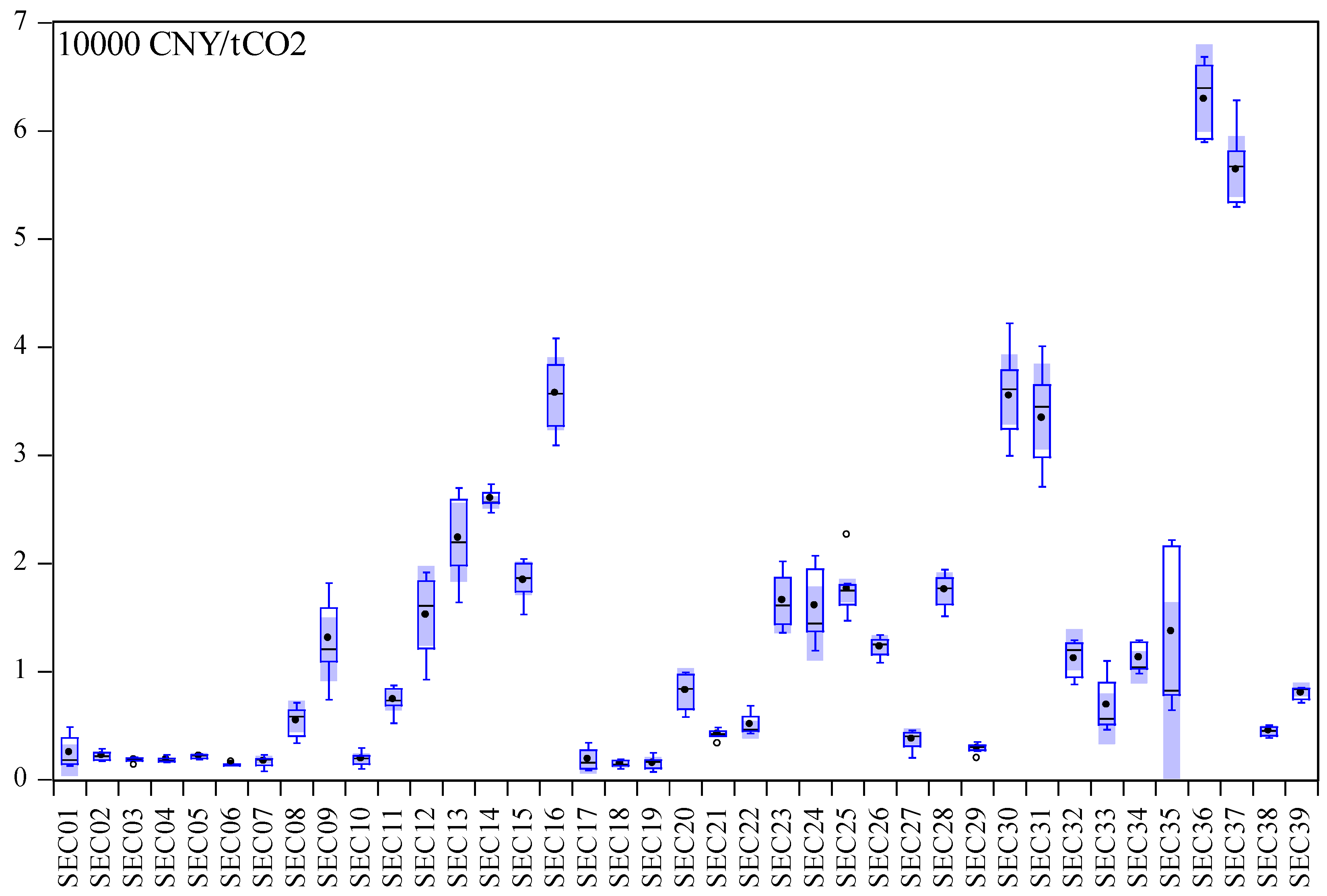
The subdivision of industry enables us to understand the MACs in industrial level. The results are shown in Figure 3 and the detailed calculation results are shown in Appendix B. There are two situations that need to be tested. First, the results in boxplots demonstrated that MACs across industries may vary dramatically. For instance, the marginal abatement costs in some sectors are markedly lower than others and the gap between the lowest one and the highest one reached 60,000 CNY/ton CO₂. In order to find out the internal causes, the carbon intensity that is most closely related to both desirable and undesirable output is taken into consideration. Furthermore, we can see that MACs in the same industry fluctuate widely over time, such as Manufacture of electrical machinery and equipment (SEC 16), Printing, reproduction of recording media (SEC 30), Manufacture of articles for culture, education and sport activity (SEC 31), Manufacture of communication equipment, computers and other electronic equipment (SEC 36), and Manufacture of measuring instruments and machinery for cultural activity and office work (SEC 37), most of which manifest a growing trend over time. Can we say with certainty that the MACs show a positive correlation with time? To verify this, we applied the kernel density function.

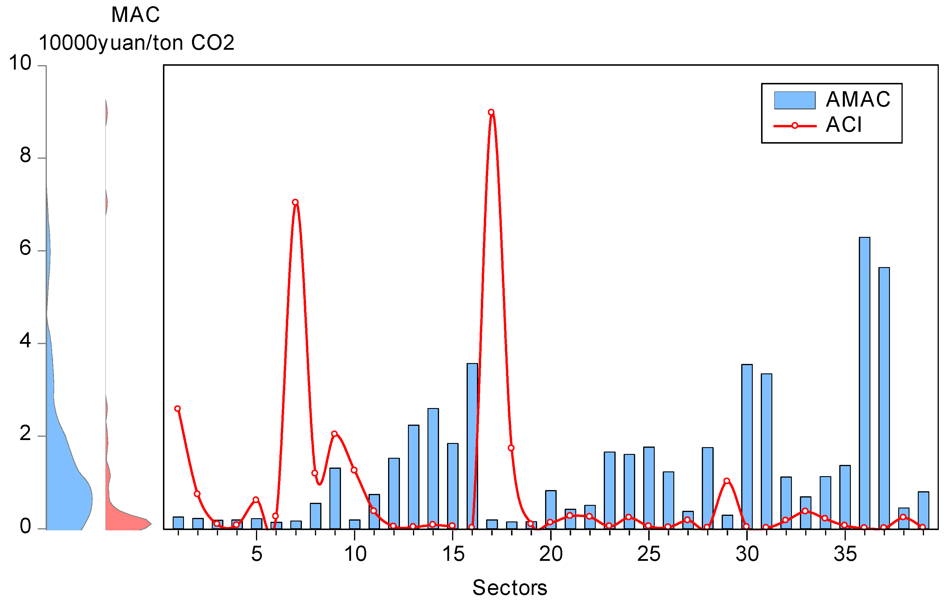
Carbon intensity, as an indicator for the relationship between carbon dioxide emissions and gross domestic product (GDP), has become a restrictive indicator used in China’s emissions reduction campaign. The average carbon intensities (denoted as ACI) from 2005 to 2011 in 39 industries are shown with red lines in Figure 4; the average MACs (denoted as AMAC) from 2005 to 2011 in 39 industries are also displayed. The vertical axis depicts the kernel probability density estimation, which is applied to estimate the density of unknown functions. The kernel density of ACI reveals that ACI mainly concentrates in 0 to 0.5 intervals, which implies that the majority of ACIs are relatively low. Nevertheless, in several sectors such as Mining and washing of coal (SEC 01), Processing of petroleum, coking, and nuclear fuel (SEC 07), and Production and distribution of electric power and heat power (SEC 17), all of which are energy-intensive industries, the ACIs are significantly higher than in others.

It is noticed that the figure roughly represents a trend that a high AMAC always occurs in an industry with a low ACI and vice versa. In other words, compared with those heavy industries, the light industries tend to have higher MACs. Although the highest ACI appeared in Production and distribution of electric power and heat power (SEC 17), its AMAC only reached 1870 CNY/ton CO₂. Conversely, Manufacture of communication equipment, computers and other electronic equipment (SEC 36), whose ACI is lowest, evidences the highest AMAC of 62,923 CNY/ton CO₂.

It is not peculiar to obtain this result. Obviously, CO₂ emissions mainly come from the use of fossil fuels. Hence, energy utilization, which is the reason for CO₂ emissions, can exert a great influence on CO₂ emissions. Given the low potential for CO₂ abatement induced by high energy efficiency, advanced energy saving technology, and relatively low energy consumption, further energy savings and emissions mitigation in those light industries would be cost-inefficient. On the contrary, energy-intensive heavy industries have relatively large flexibility in reducing CO₂ emissions owing to their lower energy efficiency and tremendously wasteful use of energy. Thus, energy saving in energy-intensive heavy industry is more promising and less costly. From the perspective of emissions reduction technology, the large-scale application of emissions reduction technology in energy-intensive industry can lead to a scale effect, which can also reduce MAC in energy-intensive industries. Additionally, a basic principle of environmental economics states that the marginal abatement cost is inversely related to emissions when the production process is inefficient, which has perfectly verified the above conclusions.

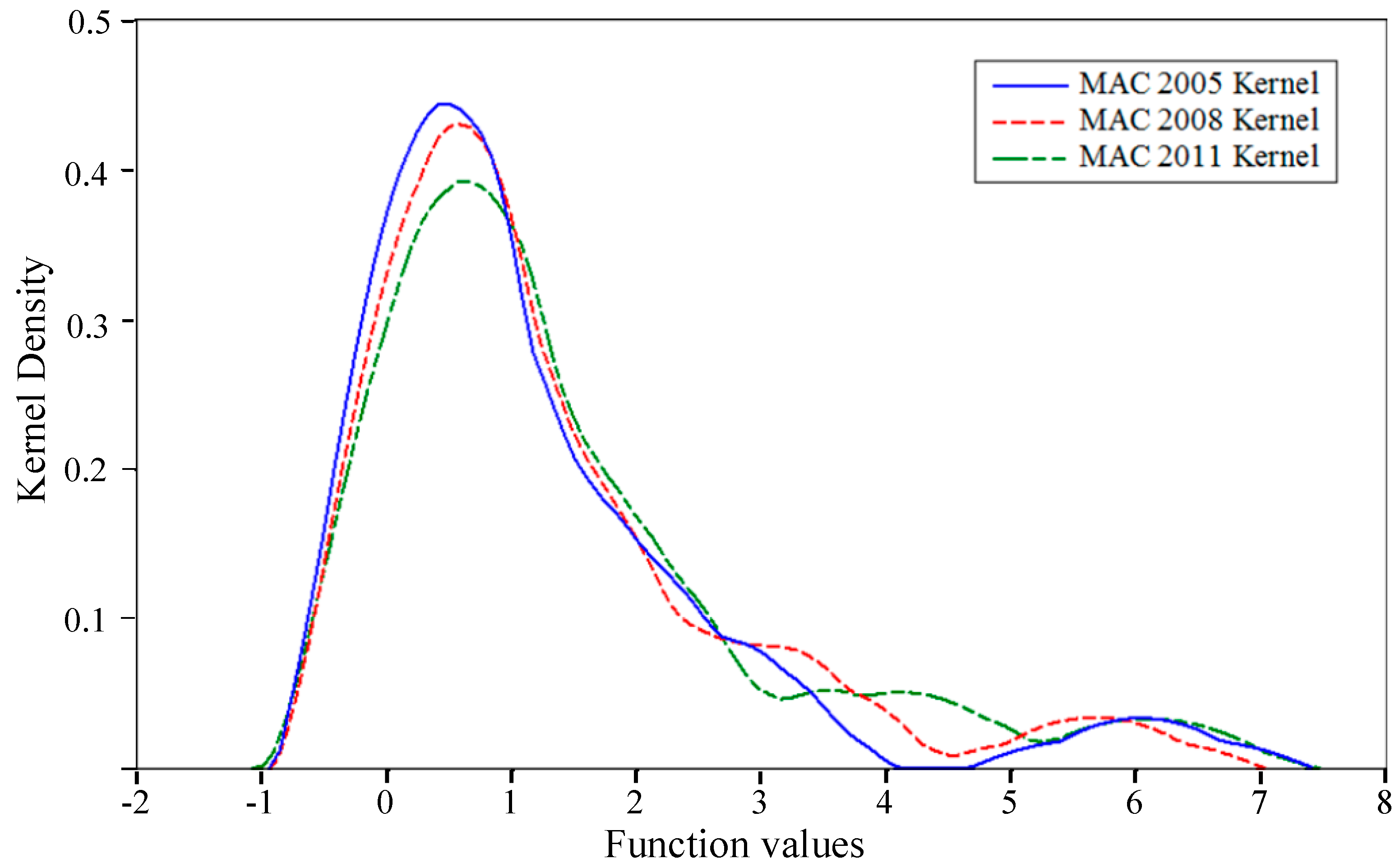
Then, in order to testify whether the MACs have a conspicuous rising tendency over time, the kernel probability density estimation is used for the second time. The kernel density of MAC in 2005, 2008, and 2011 are reported individually in Figure 5. In 2005, the MACs mainly deviate from about 0 to 10,000 CNY/ton CO₂ with the majority of the estimates clustering around the 7000 CNY/ton CO₂ mark. In 2011, the MACs deviate from about 0 to 15,000 CNY/ton CO₂, with the majority of the estimates clustering around the 9000 CNY/ton CO₂ mark.

Different from previous studies [23,42], the rightward shift of kernel density curves is not obvious enough in our research. It is co-determined by two major opposite effects. First, the space for resetting the given resources to cut CO₂ emissions is getting squeezed over time, which means that the potential for cutting CO₂ emissions will be compressed in the future. So the MAC of CO₂ emissions will inevitably go up. Meanwhile, in consideration of technology improvement, industrial structure adjustment, energy conservation measures, rational allocation of energy resources, and learning effects, the ongoing advancement of technology and learning effects, in both energy conservation and emissions reduction, can continuously lift the efficiency of the DMU and reduce the MAC of CO₂ emissions. However, large-scale technological innovations and obvious learning effects are difficult to get and spread in the short term. Hence, there is a weak increasing trend over time.

4.2. Comparative Analysis

Before a deeper analysis, the validity and rationality of the results of MACs in our paper need to be tested. Nine relevant previous studies were selected to testify the rationality of the results and find similarities between the different cases. A summary of the literature is shown in

Table 5. Summary of studies estimating MACs with distance functions.

	Research	Area/Range/Object	Sample	Methods	Weight	Value (CNY/Ton)
1	Our research	China/Industry/MAC of CO2	39	P/Q-DDF	Weighted by CO2	3517
					/	13,131
2	Yuan et al. [28]	China/Industry/MAC of CO2	24	N/DDF	/	16,360
3	Chen [42]	China/Industry/ MAC of CO2	38	P/T-DDF	/	32,687
				N/DDF	/	26,829
4	Zhou et al. [30]	Shanghai/Industry/MAC of CO2	10	P/T-SIDF	Weighted by CO2	678
				P/T-SODF	Weighted by CO2	395
				P/Q-DDF	Weighted by CO2	582
				N/DDF	Weighted by CO2	1906
5	Chen et al. [43]	Tianjin/Industry/MAC of CO2	28	N/DDF	/	766
6	Choi et al. [13]	China/Province/MAC of CO2	30	N/SBM-DEA	/	56
7	Zhang et al. [38]	China/Province/MAC of CO2	30	P/T-SODF	/	24
			30	P/Q-DDF	/	80
8	Wang et al. [39]	China/Province/MAC of CO2	28	N/DDF	/	475
9	He [44]	China/Province/MAC of CO2	29	P/T-DDF	/	104
10	Yuan and Cheng [41]	China/Nation/MAC of Waste water	/	P/Q-DDF	/	178
		China/Nation/MAC of SO2	/	P/Q-DDF	/	51,580
		China/Nation/MAC of Soot	/	P/Q-DDF	/	45,970

Note: N = Nonparametric; P = Parametric; T = Translog functional form; Q = Quadratic functional form; SODF = Shephard output distance function; SIDF = Shephard input distance function; DDF = Directional distance function; SBM = Slack-based measure; DEA = Data envelopment analysis.

.

All the previous studies can be divided into four categories. The first category is MAC of industrial sector in China; the second category is MAC of industrial sector in a certain province or region; the third is MAC at provincial level in China; and the last is the nationwide MAC. Meanwhile, the undesirable output is not limited to CO₂; other pollutants are also taken into consideration, such as SO₂, NO_x, BOD, COD, waste water, etc.

Compared with Zhou et al. [30] and Chen et al. [43], the results of our study are apparently higher than those industrial sectors in a certain province, which can be attributed to the changes in production frontier. It should also be noted that “efficiency” is the real driving factor determining the changes in production frontier, but efficiency varies dramatically within the same industry in different regions. Hence, the different results are not at all surprising in view of the tremendous differences between countries and regions. Although there are notable divergences among the results, what is noteworthy is that the trend of MACs in our paper is consistent with the relevant research. Furthermore, although MAC at a provincial level is smallest in the above studies at first sight, such estimates are not comparable due to the different objects. When analyzing our study and Yuan and Cheng [41], we can conclude that the rank of MAC for different pollutants is as follows: SO₂ > Soot > CO₂ > Waste water. This conclusion is reasonable because it is directly proportional to its negative externality.

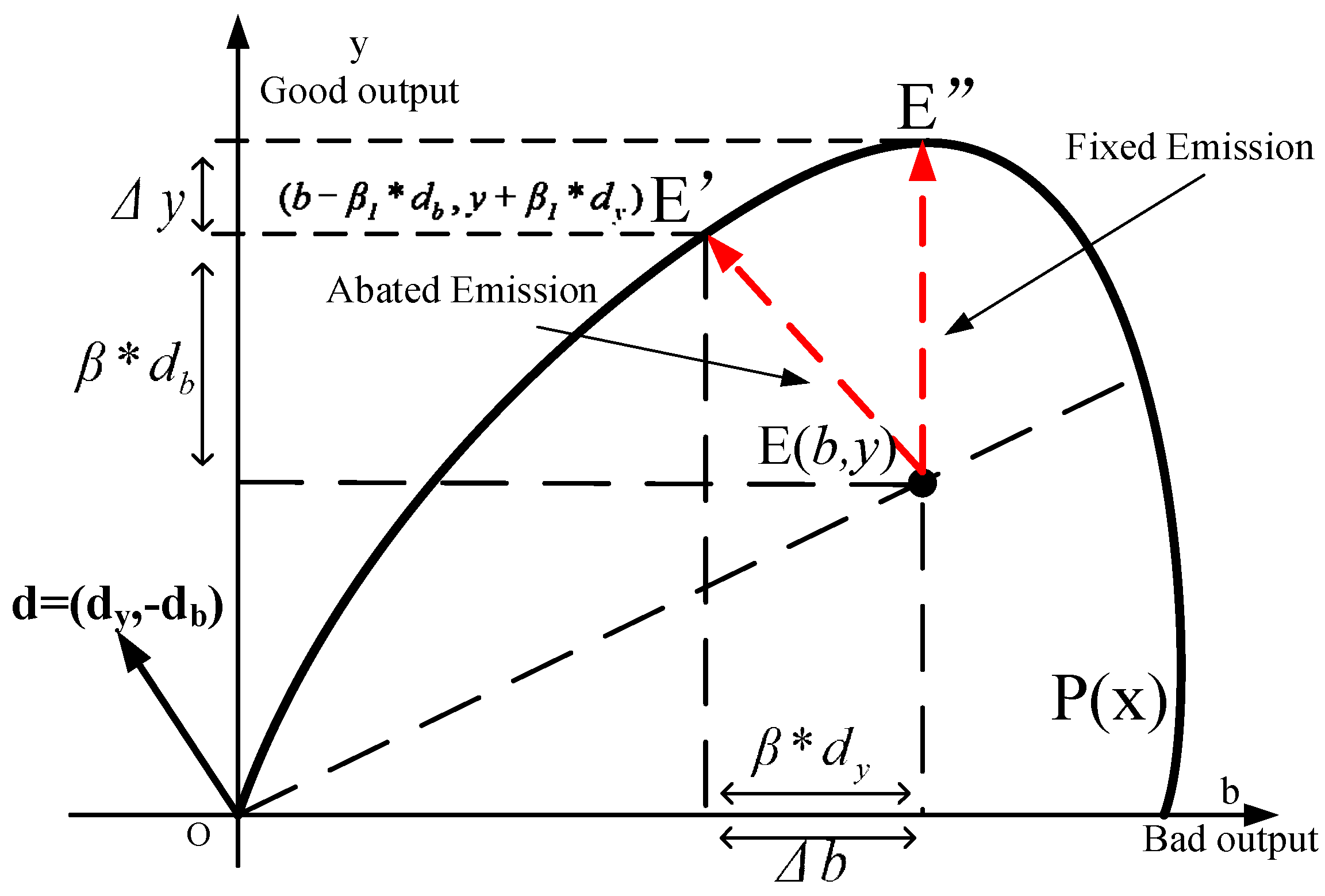
By comparing DDF (Directional distance function) and SDF (Shephard distance function), we find that the results calculated by the former method are basically larger than that of the latter. For the DMU $(b,y)$, if and only if $g=(y,-b)$, the equation ${\overrightarrow{D}}_0(x,y,b;y,-b)=1/D_0(x,y,b)-1$ ideally holds. Or, put another way, the emissions reduction path in DDF is artificially selected, whereas the path in SDF is model-driven. Different from the simultaneous expansion between desirable and undesirable outputs in the Shephard function, the directional distance function can increase economic output while cutting the growth in CO₂ emissions. Therefore, MACs calculated by DDF are greater than SDF. In addition, the direction vector, as another key factor, is a reflection of environmental policy. Generally speaking, a flat vector always corresponds to a more stringent policy environment, which means the increase in total output is accompanied by a significant reduction in CO₂ emissions.

In brief, different evaluation objects, time spans, estimation methods, and in particular, direction vectors, can significantly affect the results.

4.3. Estimation of MACC

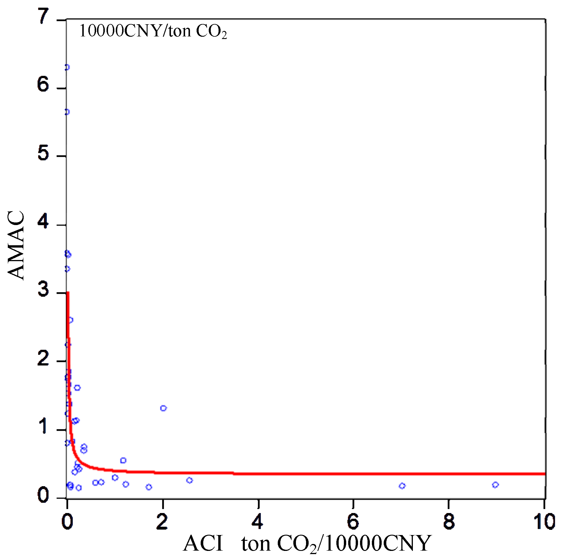
Empirically, there are commonly five kinds of non-linear functional forms, including quadratic, logarithmic, exponential, power, and hyperbolic functional forms. In order to select the optimal fitting function, the scatter diagram is shown in Figure 6.

From the above analyses, we can conclude that AMAC and ACI basically change in the reverse direction, and the marginal abatement cost curve is on a downward slope. We can observe an unambiguous nonlinear relationship between these two variables. The downward sloping curve implies that it is more costly to reduce an additional unit of CO₂ emissions for those sectors with lower carbon intensities. To estimate the relationship between the marginal abatement cost and carbon intensity, a hyperbolic function is taken into consideration. The statistics of Equation (14) are depicted in

Table 6. The regression estimates for MACC.

	F-Statistic	R-Squared	Coefficient	Standard Error	t-Statistic	Probability
a	89.129	0.696	0.0488	0.00517	9.4408	0.0000
b			0.42087	0.15711	2.6789	0.0108

.

$$MA{C}_i=a/C{I}_i+b$$

(14)

The t-statistics show that the null hypotheses for both of the parameters are overwhelmingly rejected. $F>F_{0.05}(1,39)=4.08$ means the equation passes the hypothesis testing. R-squared means the fitting equation can interpret 70% of the dependent variable changes. It is considered that this equation can be applied to explain the relationship between the MAC and CI. The function plot is depicted in Figure 6 in a red line, and its overall trend basically agrees with the sample data.

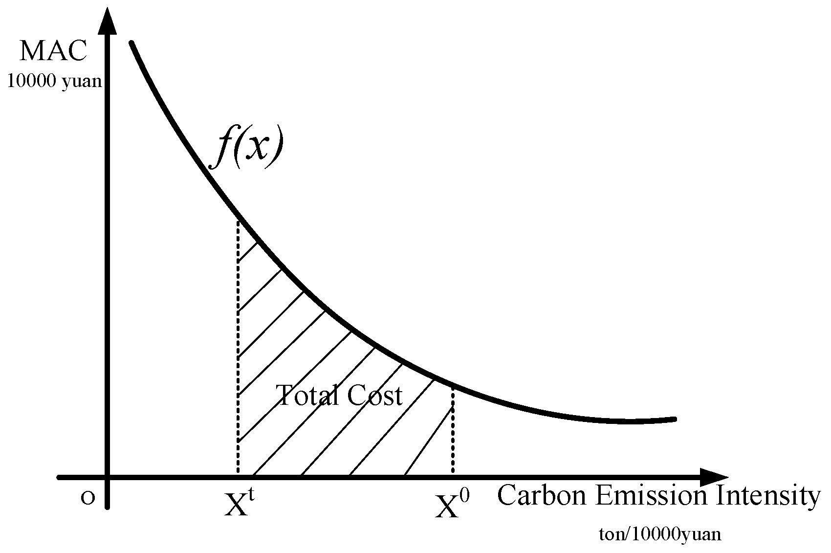
4.4. The Abatement Distribution Scheme

“The Improved Action to Address Climate Change” submitted to U.N. top climate officials by the Chinese government suggested that the peak value of carbon emissions will be achieved around 2030, and meanwhile the CO₂ emissions per unit of GDP is required to be reduced by 60%–65% compared to 2005. Affected by international commitment, an energy revolution involving emissions mitigation, improvement of energy efficiency, and transformation of the energy structure was proposed by the Chinese government. Since the nationwide emissions reduction target was issued, how to allocate the total emissions reduction target to every industry has been a burning question. Our detailed classification of industry not only enables us to look at the MACs at an industrial level, but also to seek the most applicable and optimal allocation scheme of CO₂ abatement for the Chinese government.

In this part, we calculated the abatement distribution scheme with minimum total abatement cost under four different emissions reduction targets, i.e., 5%, 10%, 15%, and 20%. The results are demonstrated in

Table 7. The abatement distribution schemes under different emissions reduction rates.

Classification	Sectors	Average MAC	Emissions Reduction Rates
			5%	10%	15%	20%
Heavy Industry	SEC 01	0.25	8.32%	12.84%	15.94%	21.84%
	SEC 02	0.222	1.65%	4.35%	13.60%	23.23%
	SEC 03	0.183	0.00%	0.00%	0.00%	3.78%
	SEC 04	0.187	0.00%	0.00%	2.62%	3.86%
	SEC 05	0.217	1.31%	2.34%	2.82%	2.72%
	SEC 06	0.141	0.00%	0.00%	6.08%	8.35%
	SEC 07	0.168	5.40%	9.95%	14.58%	21.57%
	SEC 08	0.545	1.35%	17.15%	24.81%	31.13%
	SEC 09	1.307	0.00%	1.74%	8.17%	11.48%
	SEC 10	0.191	5.26%	13.25%	21.24%	29.73%
	SEC 11	0.741	0.00%	3.72%	7.70%	11.07%
	SEC 12	1.522	0.00%	0.00%	0.00%	2.31%
	SEC 13	2.235	0.00%	0.00%	8.03%	10.47%
	SEC 14	2.598	0.00%	0.00%	1.32%	2.18%
	SEC 15	1.843	0.00%	0.00%	0.00%	1.77%
	SEC 16	3.572	0.00%	0.00%	0.00%	0.87%
	SEC 17	0.187	6.60%	11.06%	15.61%	19.25%
	SEC 18	0.15	1.96%	5.45%	11.23%	16.77%
	SEC 19	0.153	0.00%	6.43%	9.64%	13.09%
Light Industry	SEC 20	0.824	0.00%	0.00%	0.00%	3.86%
	SEC 21	0.421	0.00%	0.00%	0.00%	1.84%
	SEC 22	0.51	0.00%	0.00%	0.00%	1.98%
	SEC 23	1.656	0.00%	0.00%	0.00%	1.99%
	SEC 24	1.608	0.00%	0.00%	4.30%	5.21%
	SEC 25	1.763	0.00%	0.00%	0.00%	1.94%
	SEC 26	1.228	0.00%	0.00%	0.00%	3.27%
	SEC 27	0.373	0.00%	0.00%	0.00%	2.83%
	SEC 28	1.755	0.00%	0.00%	0.00%	2.20%
	SEC 29	0.291	0.00%	0.00%	5.43%	8.28%
	SEC 30	3.547	0.00%	0.00%	0.00%	1.42%
	SEC 31	3.342	0.00%	0.00%	0.00%	1.21%
	SEC 32	1.118	0.00%	0.00%	0.57%	1.15%
	SEC 33	0.687	0.00%	0.00%	0.27%	1.35%
	SEC 34	1.127	0.00%	0.00%	0.00%	1.40%
	SEC 35	1.369	0.00%	0.00%	0.09%	0.75%
	SEC 36	6.292	0.00%	0.00%	2.37%	2.89%
	SEC 37	5.641	0.00%	0.00%	0.00%	0.00%
	SEC 38	0.449	0.00%	0.00%	0.00%	2.10%
	SEC 39	0.798	0.00%	0.00%	0.00%	4.54%

. What is noteworthy is that the change of abatement distribution scheme is broadly consistent across the four scenarios. Therefore, we only illustrate the results under the circumstance of 20% emissions reduction.

The results show that nearly all sectors must contribute to the emissions reduction, but the emissions reduction rates vary greatly from industry to industry. Along with the transformation of China’s economic development mode, emissions reduction becomes an important task. As the focus of the national implementation of energy saving and emissions reduction, heavy industry will face greater pressure and more challenges. Mining and washing of coal (SEC 01), Extraction of petroleum and natural gas (SEC 02), Processing of petroleum, coking, and nuclear fuel (SEC 07), Manufacture of raw Chemical materials and chemical products (SEC 08), Smelting and pressing of ferrous metals (SEC 10), and Production and distribution of electric power and heat power (SEC 17), whose reduction rates reach 21.84%, 23.23%, 21.57%, 31.13% 29.73%, and 19.25%, respectively, are the six main energy saving and pollution emissions reduction industries. Moreover, besides the above six sectors, there are several sectors whose reduction rates are maintained above 10%, i.e., Manufacture of non-metallic mineral products (SEC 09), Smelting and pressing of non-ferrous metals (SEC 11), Manufacture of general purpose machinery (SEC 13), Production and distribution of gas (SEC 18), and Production and distribution of water (SEC 19). The rest contribute poorly to the abatement, with an emissions reduction rate below 10%.

These findings are understandable. First, as for those sectors with high emissions reduction proportions, they are a group with something in common—lower MACs and higher carbon intensities. Under a circumstance of 20% nationwide emissions reduction target, the allocated emissions reduction rate in Manufacture of raw chemical materials and chemical products (SEC 08) reaches 31.13%, ranking first. Undoubtedly, low MACs and a large amount of energy consumption in these sectors result in a promising future in CO₂ reduction. Then, the question arises: why does the Production and distribution of electric power and heat power (SEC 17), whose carbon intensity is highest, not make the greatest contribution to emissions reduction? The electric and heat power industry, which relies heavily on coal, has its own particularity. The reason can be traced back to inter-links between upstream and downstream industries. Apparently, it is a downstream industry of the coal sector and upstream of most economic sectors. Emissions reduction is subject to the conditions of upstream and downstream industries. To put it another way, big cuts in CO₂ emissions may induce capacity cutting and price booming, which can induce a contracting demand upstream and rising cost downstream. The co-effects of upstream and downstream constrained the potential for emissions reduction in the electric and heat power industry.

Compared with those industries that have high emissions reduction rates, the emissions reduction rates in light industries and some equipment manufacturing industries are lower than 10%. Among them, the lowest emissions reduction rate appears in Manufacture of measuring instruments and machinery for cultural activity and office work (SEC 37), which scarcely contribute to the emissions reduction. These industries should not become the focus of the emissions reduction; otherwise society will pay a high cost.

5. Conclusions and Policy Implications

Looking back to this paper’s research questions, this paper tries to calculate the MACs of CO₂ in China’s industrial level. The directional distance function combined with panel data covering 39 sectors for the period 2005–2011 were used. Additionally, a MACC was established to reflect the association between marginal abatement cost and carbon intensity. Moreover, we set up a model to measure the abatement distribution scheme with minimum cost. The conclusions are as follows.

The results of this paper show that MACs vary greatly from industry to industry; high MACs always occur in industries with low carbon intensity and vice versa. Additionally, the rightward shift of kernel density curves is not obvious enough in our research. The space for resetting the given resources to cut CO₂ emissions is getting squeezed over time. Meanwhile, the ongoing advancement of technology and learning effects, in both energy conservation and emissions reduction, can continuously lift the efficiency of DMU and cut the MAC of CO₂ emissions. These two major, opposite effects ensure that there is a weak increasing trend over time in MACs. To establish the MACC, a hyperbolic function is set up to estimate the relationship between the carbon intensity and MAC. The downward sloping curve means that it is more costly to reduce an additional unit of CO₂ emissions for sectors with lower carbon intensity. Furthermore, this paper addresses the importance of an abatement distribution scheme. The results of the abatement distribution scheme indicate that those heavy industries with low MACs and high carbon intensities should shoulder the responsibility for emissions reductions, and those light industries with high MACs should not become the focus of the emissions reduction; otherwise society will pay a high cost.

The above conclusions theoretically provide information for stakeholders and policymakers to shape optimal policy schemes for reducing CO₂ emissions. However, a deep analysis of the policy implications is necessary. Hence, some policy implications for how to apply the MAC are as follows.

(1)

Clean Development Mechanism (CDM), as one of the flexible mechanisms of the Kyoto Protocol, plays a decisive role in the European Union Emissions Trading Scheme (EU ETS). At present, although China has become the biggest exporter of CDM, there is still a lack of pricing power on CDM. The largest buyer, the European Union, predominantly influences the price of certified emissions reductions (CERs), which results in a huge gap between the final transaction price and the international market price and the loss of carbon assets in China. Measuring the emissions reduction cost can help the Chinese government increase the voice of China in the field of EU ETS.

(2)

The MAC of environmental pollution is the cornerstone of environmental policy, or, more precisely, it can provide reliable evidence for carbon tax. A high carbon tax will increase the financial burden of enterprises and a low carbon tax will have a weak effect on environmental dividends. The MAC of CO₂ in this paper reflects the real cost of CO₂ reduction and provides a reference for the Chinese government’s policy decisions on carbon tax.

(3)

MAC can represent the MRTS (Marginal Rate of Technical Substitution) of the undesirable outputs for desirable outputs. i.e., $MRTS=\Delta y/\Delta b=MAC$. Therefore, according to the MAC in industrial level, the government can assess the impact of short-term output changes on environmental quality in a certain sector.

(4)

Under the market mechanism, various sectors will determine their emissions reduction behaviors based on their own abatement costs. Due to the distinctness of an industry’s features and development, a “one size fits all” traditional abatement distribution approach is obsolete. “Differential treatment” is critical while developing and implementing carbon reduction policies. What the results of an abatement distribution scheme mean for policy is that heavy industries with low MACs should take more responsibility for emissions reduction and vice versa.

References

1. Michael, J. IPCC fifth assessment synthesis report: “Climate change 2014: Longer report”: Critical analysis. Technol. Forecast. Soc. Chang. 2015, 92, 362–363. [Google Scholar]
2. Edenhofer, O.; Seyboth, K. Encyclopedia of Energy, Natural Resource, and Environmental Economics; Elsevier: Waltham, UK, 2013; pp. 48–56. [Google Scholar]
3. Zhou, K.; Yang, S.; Shen, C.; Ding, S.; Sun, C. Energy conservation and emission reduction of China’s electric power industry. Renew. Sustain. Energy Rev. 2015, 45, 10–19. [Google Scholar] [CrossRef]
4. Wu, J.; Lv, L.; Sun, J.; Ji, X. A comprehensive analysis of China’s regional energy saving and emission reduction efficiency: From production and treatment perspectives. Energy Policy 2015, 84, 166–176. [Google Scholar] [CrossRef]
5. Chen, A.; Groenewold, N. Emission reduction policy: A regional economic analysis for China. Econ. Model. 2015, 51, 136–152. [Google Scholar] [CrossRef]
6. Zhang, Y.; Wei, Y.M. An overview of current research on EU ETS: Evidence from its operating mechanism and economic effect. Appl. Energy 2010, 87, 1804–1814. [Google Scholar] [CrossRef]
7. Cui, L.; Fan, Y.; Zhu, L.; Bi, Q. How will the emissions trading scheme save cost for achieving China’s 2020 carbon intensity reduction target? Appl. Energy 2014, 136, 1043–1052. [Google Scholar] [CrossRef]
8. Chiu, F.; Kuo, H.; Chen, C.; Hsu, C. The energy price equivalence of carbon taxes and emissions trading—Theory and evidence. Appl. Energy 2015, 160, 164–171. [Google Scholar] [CrossRef]
9. Guo, Z.; Zhang, X.; Zheng, Y.; Rao, R. Exploring the impacts of a carbon tax on the Chinese economy using a CGE model with a detailed disaggregation of energy sectors. Energy Econ. 2014, 45, 455–462. [Google Scholar] [CrossRef]
10. Mo, J.L.; Agnolucci, P.; Jiang, R.M.; Fan, Y. The impact of Chinese carbon emission trading scheme (ETS) on low carbon energy (LCE) investment. Energy Policy 2016, 89, 271–283. [Google Scholar] [CrossRef]
11. Zhou, P.; Zhou, X.; Fan, L.W. On estimating shadow prices of undesirable outputs with efficiency models: A literature review. Appl. Energy 2014, 130, 799–806. [Google Scholar] [CrossRef]
12. Teng, F.; Wang, X.; Pan, X.; Yang, X. Understanding Marginal Abatement Cost Curves in Energy-intensive industries in China: Insights from Comparison of Different models. Energy Procedia 2014, 61, 318–322. [Google Scholar] [CrossRef]
13. Choi, Y.; Zhang, N.; Zhou, P. Efficiency and abatement costs of energy-related CO2 emissions in China: A slacks-based efficiency measure. Appl. Energy 2012, 98, 198–208. [Google Scholar] [CrossRef]
14. Liu, Y.; Lu, Y. The Economic impact of different carbon tax revenue recycling schemes in China: A model-based scenario analysis. Appl. Energy 2015, 141, 96–105. [Google Scholar] [CrossRef]
15. Simões, S.; Cleto, J.; Fortes, P.; Seixas, J.; Huppes, G. Cost of energy and environmental policy in Portuguese CO2 abatement-scenario analysis to 2020. Energy Policy 2008, 36, 3598–3611. [Google Scholar] [CrossRef]
16. Gao, P.; Chen, W.; He, J. China’s marginal cost of carbon dioxide. J. Tsinghua Univ. Sci. Technol. 2004, 9, 1192–1195. (In Chinese) [Google Scholar]
17. Tomaschek, J. Marginal abatement cost curves for policy recommendation—A method for energy system analysis. Energy Policy 2015, 85, 376–385. [Google Scholar] [CrossRef]
18. Gómez-Calvet, R.; Conesa, D.; Gómez-Calvet, A.R.; Tortosa-Ausina, E. Energy efficiency in the European Union: What can be learned from the joint application of directional distance functions and slacks-based measures? Appl. Energy 2014, 132, 137–154. [Google Scholar] [CrossRef]
19. Färe, R.; Grosskopf, S.; Lovell, C.A.; Yaisawarng, S. Derivation of shadow prices for undesirable outputs: A distance function approach. Rev. Econ. Stat. 1993, 75, 374–380. [Google Scholar] [CrossRef]
20. Färe, R.; Grosskopf, S.; Noh, D.W.; Weber, W. Characteristics of a Polluting Technology: Theory and Practice. J. Econom. 2005, 126, 469–492. [Google Scholar] [CrossRef]
21. Färe, R.; Primont, D. Multi-Output Production and Duality: Theory and Applications; Kluwer Academic: Dordrecht, The Netherlands, 1995. [Google Scholar]
22. Färe, R.; Grosskopf, S. Theory and application of directional distance functions. J. Product. Anal. 2000, 13, 93–103. [Google Scholar] [CrossRef]
23. Du, L.; Hanley, A.; Wei, C. Estimating the Marginal Abatement Cost Curve of CO2 Emissions in China: Provincial Panel Data Analysis. Energy Econ. 2015, 48, 217–229. [Google Scholar] [CrossRef]
24. Islas, J.; Grande, G. Abatement costs of SO2-control options in the Mexican electric-power sector. Appl. Energy 2008, 85, 80–94. [Google Scholar] [CrossRef]
25. Lee, M.; Zhang, N. Technical efficiency, shadow price of carbon dioxide emissions, and substitutability for energy in the Chinese manufacturing industries. Energy Econ. 2012, 34, 1492–1497. [Google Scholar] [CrossRef]
26. Lee, M. Potential cost savings from internal/external CO2 emissions trading in the Korean electric power industry. Energy Policy 2011, 39, 6162–6167. [Google Scholar] [CrossRef]
27. Ke, T.Y.; Hu, J.L.; Li, Y.; Chiu, Y.H. Shadow prices of SO2 abatements for regions in China. Agric. Resour. Econ. 2008, 5, 59–78. [Google Scholar]
28. Yuan, P.; Liang, W.; Cheng, S. The Margin Abatement Costs of CO2 in Chinese industrial sectors. Energy Procedia 2012, 14, 1792–1797. [Google Scholar]
29. Aparicio, J.; Pastor, J.T.; Vidal, F. The directional distance function and the translation invariance property. Omega 2016, 58, 1–3. [Google Scholar] [CrossRef]
30. Zhou, X.; Fan, L.W.; Zhou, P. Marginal CO2 abatement costs: Findings from alternative shadow price estimates for Shanghai industrial sectors. Energy Policy 2015, 77, 109–117. [Google Scholar] [CrossRef]
31. Molinos, S.M.; Hanley, N.; Sala, G.R. Measuring the CO2 shadow price for wastewater treatment: A directional distance function approach. Appl. Energy 2015, 144, 241–249. [Google Scholar] [CrossRef]
32. Duan, N.; Guo, J.; Xie, B. Is there a difference between the energy and CO2 emission performance for China’s thermal power industry? A bootstrapped directional distance function approach. Appl. Energy 2016, 162, 1552–1563. [Google Scholar] [CrossRef]
33. Charnes, A.; Cooper, W.W.; Rhodes, E. Measuring the efficiency of decision making units. Eur. J. Oper. Res. 1978, 2, 429–444. [Google Scholar] [CrossRef]
34. Turner, J. Measuring the Cost of Pollution Abatement in the Electric Utility Industry: A Production Function Approach. Ph.D. Dissertation, University of North Carolina, Chapel Hill, NC, USA, 1994. [Google Scholar]
35. Leleu, H. Shadow pricing of undesirable outputs in nonparametric analysis. Eur. J. Oper. Res. 2013, 231, 474–480. [Google Scholar] [CrossRef]
36. Mekaroonreung, M.; Johnson, A.L. A nonparametric method to estimate a technical change effect on marginal abatement costs of U.S. coal power plants. Energy Econ. 2014, 46, 45–55. [Google Scholar] [CrossRef]
37. Chang, T.P.; Hu, J.L. Total-factor energy productivity growth, technical progress, and efficiency change: An empirical study of China. Appl. Energy 2010, 87, 3262–3270. [Google Scholar] [CrossRef]
38. Zhang, X.; Xu, Q.; Zhang, F.; Guo, Z.; Rao, R. Exploring shadow prices of carbon emissions at provincial levels in China. Ecol. Indic. 2014, 46, 407–414. [Google Scholar] [CrossRef]
39. Wang, Q.; Cui, Q.; Zhou, D.; Wang, S. Marginal abatement costs of carbon dioxide in China: A nonparametric analysis. Energy Procedia 2011, 5, 2316–2320. [Google Scholar] [CrossRef]
40. Kaneko, S.; Fujii, H.; Sawazu, N.; Fujikura, R. Financial allocation strategy for the regional pollution abatement cost of reducing sulfur dioxide emissions in the thermal power sector in China. Energy Policy 2010, 38, 2131–2141. [Google Scholar] [CrossRef]
41. Yuan, P.; Cheng, S. Estimating shadow pricing of industrial pollutions in China. Stat. Res. 2011, 9, 66–73. (In Chinese) [Google Scholar]
42. Chen, S. The shadow price of CO2 in industrial sectors: Parametric and nonparametric methods. World Econ. 2010, 8, 93–111. (In Chinese) [Google Scholar]
43. Chen, L.; Liu, J.; Wang, X.; Zhang, Z. Marginal carbon abatement cost estimation based on the DDF dynamic analysis model-Taking Tianjin for example. Syst. Eng. 2014, 9, 74–80. (In Chinese) [Google Scholar]
44. He, X. Regional differences in China’s CO2 abatement cost. Energy Policy 2015, 80, 145–152. [Google Scholar] [CrossRef]
Figure 1. Diagram of directional distance function.
Sustainability 09 00138 g001
Figure 2. Marginal abatement cost curve.
Sustainability 09 00138 g002
Figure 3. The calculation results of industrial MACs in 2005–2011.
Sustainability 09 00138 g003
Figure 4. The average MAC and CI.
Sustainability 09 00138 g004
Figure 5. Kernel density of the MAC estimates.
Sustainability 09 00138 g005
Figure 6. The scatter diagram and regression curve of MAC estimates.
Sustainability 09 00138 g006