Prediction of Climate Change Induced Temperature & Precipitation: The Case of Iran

Abstract

Concern about the effects of climatic change on numerous aspects of human life in general and on agricultural production in particular is growing. The utility of HadCM3 as a tool in climate change predictions in cross cultural studies is scarce. Therefore, this study sought to investigate and predict climate change induced temperature and precipitation in Iran. The calibration and validation using the HadCM3 was performed during 1961–2001, using daily temperatures and precipitation. The data on temperature and precipitation from 1961 to 1990 were used for calibration, and, for model validation, data from 1991 to 2001 were used. Moreover, in order to downscale general circulation models to station scales, SDSM version 4.2 was utilized. The least difference between observed data and simulation data during calibration and validation showed that the parameter was precisely modeled for most of the year. Simulation under the A2 scenario was performed for three time periods (2020, 2050, and 2080). According to our simulated model, precipitation showed a decreasing trend whereas temperature showed an increasing trend. The result of this research paper makes a significant contribution to climate smart agriculture in Iran. For example, rural development practitioners can devise effective policies and programs in order to reduce the vulnerability of local communities to climate change impacts. Moreover, the result of this study can be used as an optimal model for land allocation in agriculture. Moreover, a shortage of rainfall and decreased temperatures also have implications for agricultural land allocation.

1. Introduction

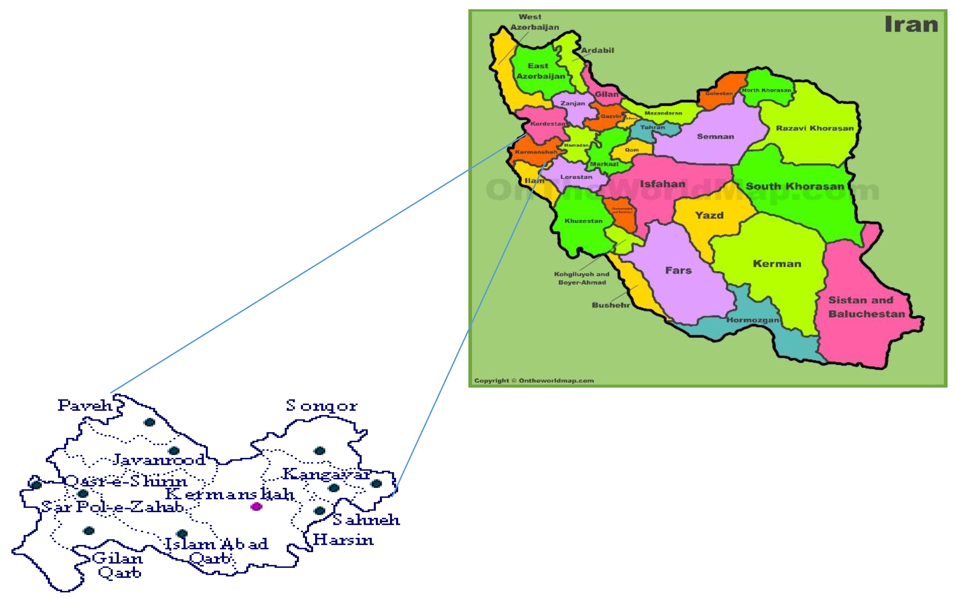
Iran is home to 77 million people [1], with an area of 1,648,000 km². It has 1.1% of the global population and is located in an arid and semi-arid region with a yearly average precipitation of 250 mm [2]. Iran is located in south-west Asia in the arid belt of the world. About 60% of the country is mountainous and the remaining part (1/3) is deserts and arid lands. The country has a diverse climatic condition across provinces with significant rainfall variability. The northern and western provinces experience an average rainfall of 2000 mm per year, whereas the central and eastern provinces of the country receive an average rainfall of 120 mm per year. Moreover, the minimum and maximum temperatures in the southwest region reach as low as −20 °C and as high as 50 °C across the Persian Gulf. Concern about the effects of climatic change on numerous aspects of human life in general and on agricultural production in particular is growing. As an example, at farm level, information on climate variability can be used for planning future crop patterns and the prediction of climate change can aid farmer resilience when adapting to climate variability. Moreover, the finding of this study has implications for climate smart agriculture (CSA) in Iran. For example, predictions of climate change induced temperature and precipitation aid rain-fed farmers to take proactive measures when selecting cultivars and planning for water resource management.

Currently, there are several models for predicting climate change. For example, when the focus is to predict climate under elevated CO₂ concentration, General Circulation Models (GCMs) are more appropriate to use [2]. When coarse spatial resolution is the objective of the climate change information, General Circulation Models are considered to be the most reliable source [3]. Some of the most famous general circulation models are HadCM3, PCMI, MPI, CGCM3, and CSIRO-MK2 [4]. HadCM3 (Hadley Centre Coupled Model) is an Atmosphere-Ocean General Circulation Model (AOGCM) developed at the Hadley Centre in the United Kingdom. Interestingly, the Third Assessment Report of IPCC in 2001 used an AOGCM as its major model to predict climate change [5]. Thus far, in Iran, the prediction of climate change has been conducted using PCMI, MPI, CGCM3, and CSIRO-MK2 [2,6,7,8]. However, research on predicting climate change using HadCM3 is less common in Iran.

In this research, HadCM3, under the A2 emission scenario, is used. The main advantage of using HadCM3 over BCM2, ECHO-G, CGCM2, or ECHAM4 is its compatibility in cross-cultural studies as well as its high resolution (Atmosphere: 2.5 × 3.75 degrees lat-lon resolution, 19 vertical levels, 30 min time step for dynamics, 3 h for radiative transfer; Ocean: 1.25 × 1.25 degrees lat-lon resolution, 20 vertical levels, 1 h time step). Moreover, due to the large scale of the models, downscaling is deemed important. Downscaling, in general, is defined as a relationship creator factor between large-scale cycles (predictors) and the climate variables at the local scale (predictands) [9]. Most researchers apply several downscaling techniques when they are faced with the GCM outputs [10,11,12,13,14,15]. In this study the Statistical Downscaling Model (SDSM) suggested by Wilby et al. [16] was used. Furthermore, this model is based on multiple linear regression.

There are several research studies related to assessing and predicting climate change using the HadCM3 model. Therefore, in this section, we will focus on studies that have used HadCM3 for predicting climate change. Kazemi Rad and Mohammadi [7] presented two models of HadCM3 and MPEh5 for predicting climate change in Gilan Province. The results revealed that mean precipitation would decrease for 2011–2030. Moreover, during the model validation process, the mean monthly precipitation, minimum and maximum temperature, and solar radiation were correlated at a 0.05 level of confidence.

Nury and Alam [17] showed the utility of the statistical downscaling model to assess the output of the HadCM3 in Bangladesh. They worked with temperature and rainfall data and found statistical downscaling of GCMs to be an effective tool in minimizing the impacts of climate change. Furthermore, they concluded that the performance of HadCM3 downscaled by SDSM is acceptable for temperature and precipitation. They also suggested that GCMs can effectively be used when there are missing temperature and precipitation data. Johns et al. [18] used an improved coupled model of HadCM3 and concluded that the Mid-USA and Southern Europe regions will eventually tend to become slightly wetter while Australia becomes drier.

Tate et al. [8] applied HadCM3 to run a water balance sensitivity analysis in Lake Victoria towards climate change under two different emission scenarios (A2 and B2). The results revealed a significant change in annual rainfall and evaporation. They further predicted a decline in water levels during 2021–2050. However, the result of their study did not support the projected increase in water levels later in the century (2070–2099). Taie Semiromi et al. [19] sought to investigate the impacts of climate change on the groundwater stored above the discharge level using groundwater depletion analysis in the Bar watershed in Iran. Results showed that, for SRES A2, the HadCM3/LARS-WG predicted that the mean annual, maximum, and minimum temperatures will rise by 1.1, 3.2, and 4.6 °C and precipitation will decrease by 16.4%, 17.6%, and 31.4% during the projected periods of 2010–2039, 2040–2069, and 2070–2099 respectively, compared to the base period of 1970–2010.

The predictive changes in the distribution and frequency of cereal aphids in Canada using a mechanistic mathematical model was assessed by Jonathan [20]. Although HadCM3 projections predicted an abundance of latitudinal shifts northward with longitudinal variations, when used with the CGCM2 projections, the summer cereal aphid population showed a declining trend in the continental region, while the coastal region showed an increasing trend.

Valizadeh et al. [21] studied the impact of future climate change on several characteristics of wheat production in Iran. These characteristics were the period of maturity, the Leaf Area Index (LAI), biomass, and grain yield. They utilized two general circulation models (HadCM3 and IPCM4) under three scenarios (A1, B1, and A2) in three different time periods (2020, 2050, and 2080). Results demonstrated that there will be a significant decrease in wheat production in the study area. They further recommended that more mitigation strategies such as crop rotation are required if wheat growers are to become more resilient to the adverse effect of future climate change.

Sayari et al. [14] used historical data during 1984–2005 to assess the relationships between evapotranspiration and crop performance in the Kashafrood Basin in Northeast Iran. They used HadCM3 downscaled outputs to predict precipitation and temperature under the A2 scenario and an ASD (Automated Statistical Downscaling) model. Results revealed a projected annual precipitation increase of 4.64%, 5.41%, and 2.22% for 2010–2039, 2040–2069, and 2070–2099, respectively. De Silva [22] determined the impact of climate change on soil moisture in Sri Lanka. He used data from the outputs of a HadCM3 model for selected IPCC SRES scenarios for 2050. The selected data was further compared with the baseline data from the International Water Management Institute (IWMI). The prediction revealed a slight increase in the annual average rainfall due to an increase in rainfall during the southwest monsoon. The study further concluded that there would be a reduction in the east monsoon precipitation but an increase in the annual average temperature. More related studies can be found in the literature, e.g., [16,23,24,25,26].

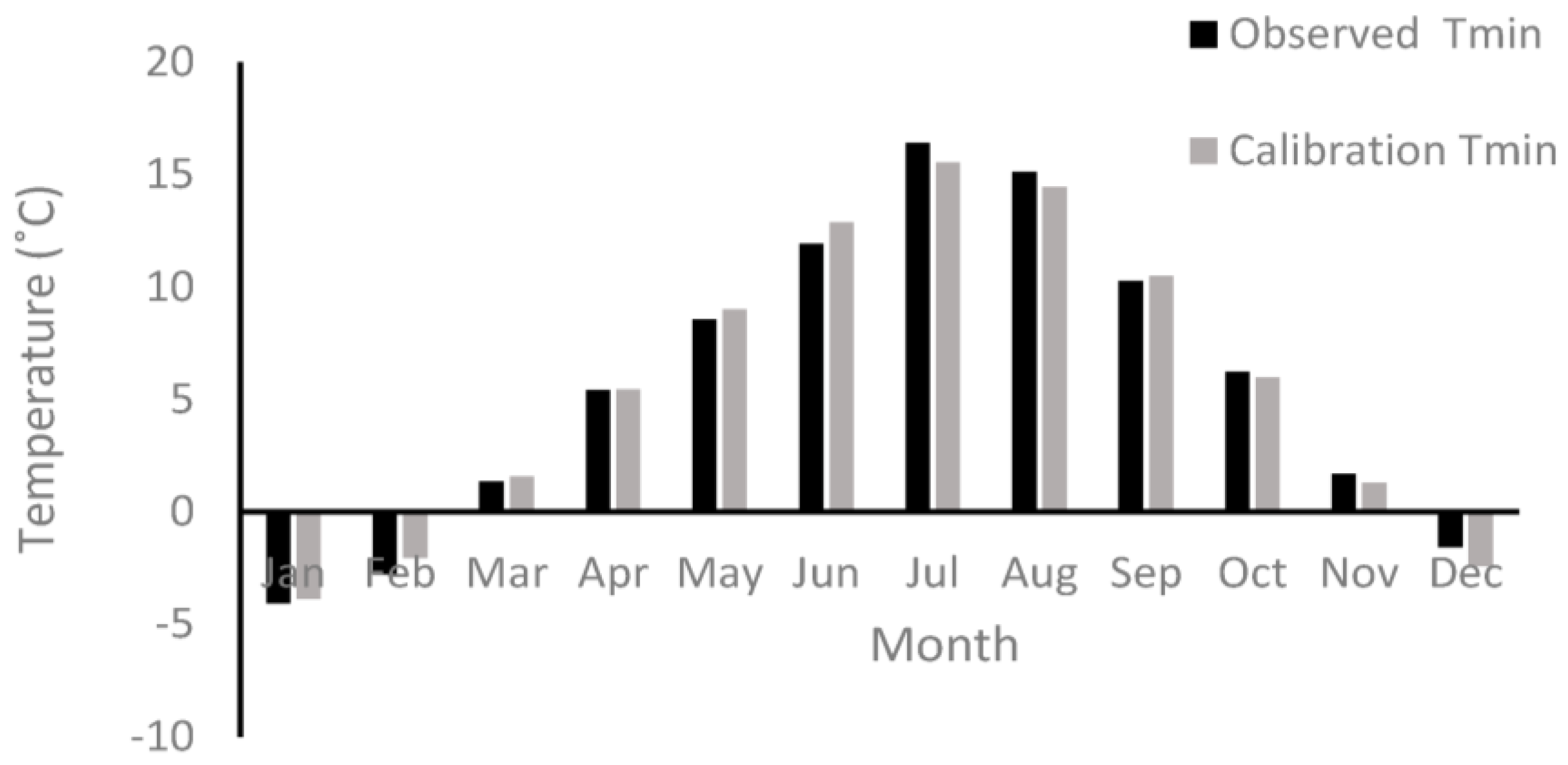
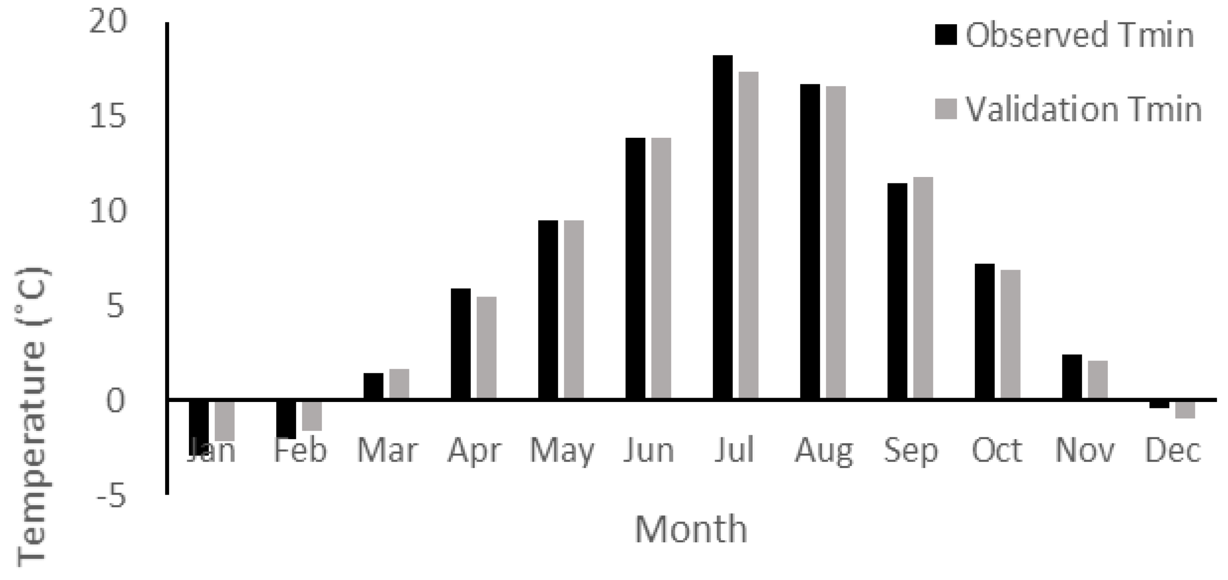
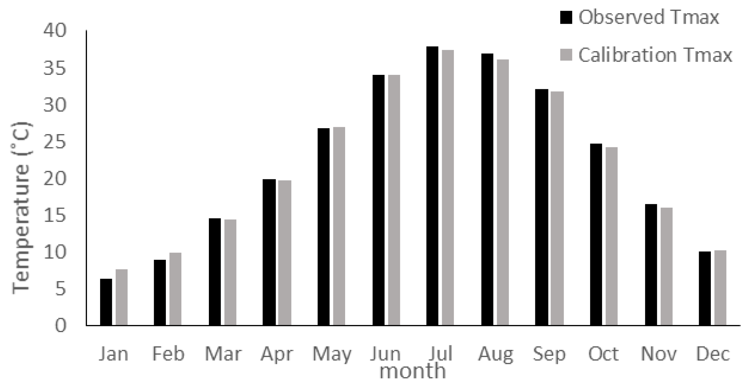
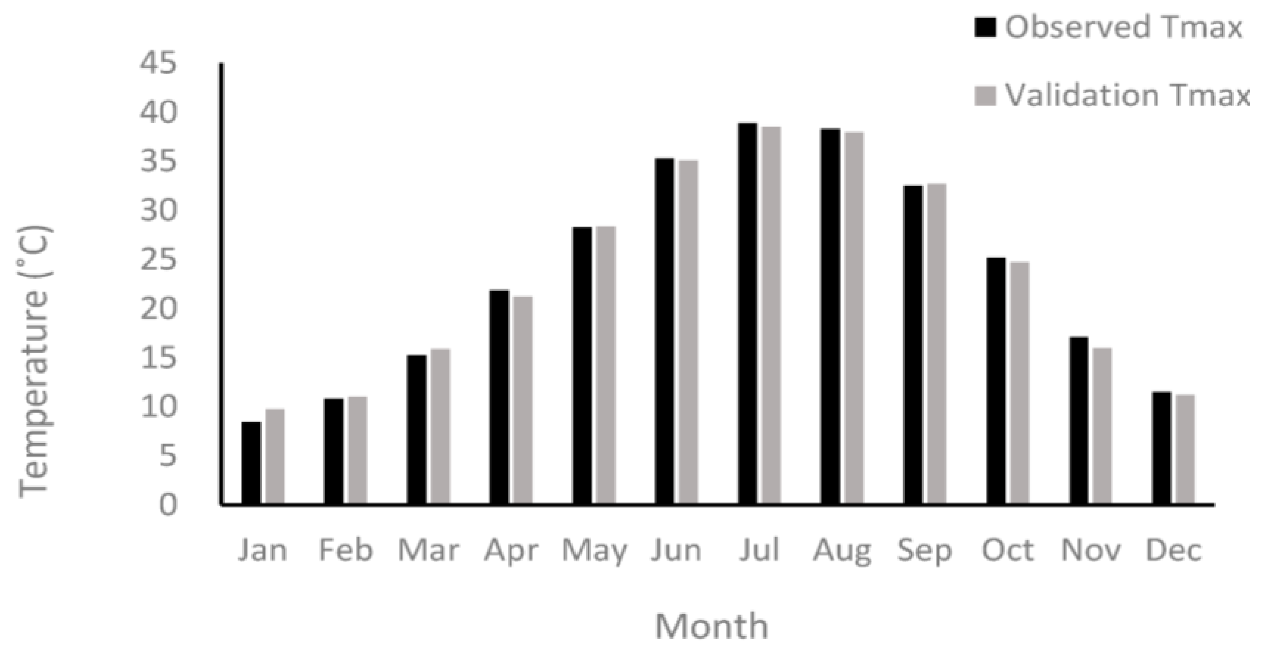
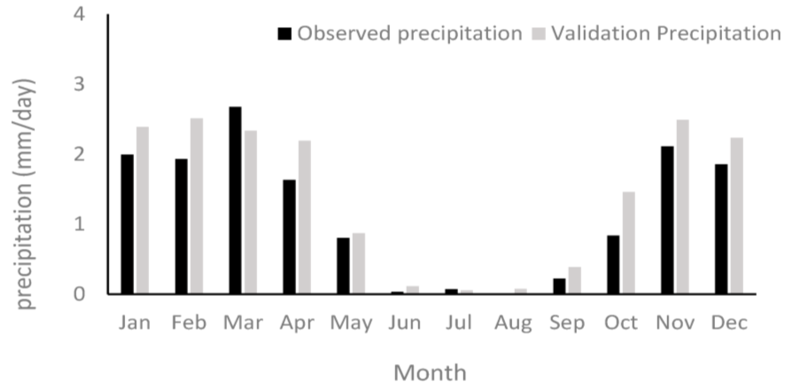
The main purpose of this study is to assess and predict potential future climate change induced temperature and precipitation on a regional scale for the Kermanshah synoptic station. The paper is organized as follows. After the introduction, the study area and data collection are described. Next, the methodology is presented, discussing the ability of HadCM3 and SDSM to simulate climate parameters and explaining how future climate scenarios are generated. In the results and discussion section, the performance of HadCM3 and SDSM for simulating climate parameters is evaluated and predictions of future climate scenarios are presented and discussed. Conclusions are presented in the last part.

2. Materials and Methods

2.1. Study Area Description and Data Collection

Figure 1 shows the study area, comprised of the Kermanshah township, which has a total area of 5658.4 m² and is located in the western part of Iran. It is subdivided into thirteen counties including Sanjabi, Razavar, Jalalvand, Baladarband, Miandarband, Alayarkhani, Mahidasht, Faraman, Firoozabad, Osmanvand, Haftashyan, Gharesoo, and Jaghanarges. The Kermanshah township is located between latitudes 33°37′N and 35°17′N and longitudes 45°20′E and 48°1′E. The yearly average precipitation of the Kermanshah township is about 456.8 mm, the mean annual temperature is 14 °C, and the average relative humidity is over 40% [1]. Agriculture is the primary source of livelihood and contributes significantly to the food production in Kermanshah Province. The population of the Kermanshah township was 851,405 in 2016, with 20.6% involved in agricultural production. The main crops grown in the township are wheat, barley, canola, corn, and sugerbeets [1].

2.2. GCM-Downscaled Climate Change Predictions for the Study Region

Climate models are numerical tools that are used for studying global, regional, or local climate. However, due to the changing conditions of the earth, several diverse climate models with different forms have been developed. These models are further categorized into simple (energy balance), intermediate (earth system), and comprehensive (global climate). The physical and mathematical characteristics of these models account for the interrelationships between diverse sections of climate systems in the biosphere, hydrosphere, cryosphere, atmosphere, and geosphere [9]. However, GCMs are limited in that they are not appropriate for providing information at finer scales, thus making them appropriate for local climate impact assessments. This, of course, is not the case for the computational grid (typically of the order of 100–200 km) and processes. In order to overcome these limitations, different downscaling techniques such as dynamic and statistical models are proposed [13]. The downscaling method used in this study is SDSM (Statistical Downscaling Model) [16]. The SDSM includes multivariate analysis, a multiple stochastic weather generator, and weather classification schemes. In the first step, the model has been calibrated and validated for simulation weather data using observed data and data from the National Centers for Environmental Prediction (NCEP). When the SDSM is calibrated, it is further used to downscale HadCM3 data in order to obtain 20 ensembles of synthetic daily precipitation and temperatures for baseline and future periods. The baseline period spans from 1961 to 1990, while the future period included 2010–2039, 2040–2069, and 2070–2099 (denoted as 2020s, 2050s, and 2080s, respectively). Among diverse emission scenarios, the A2 scenario deals with less developed countries that seek technological advancement. Moreover, the A2 scenario follows sustainable development with a greater emphasis on environmental issues.

In the next and final step, the influence of potential climate change on weather parameters is measured. In this step, we attempted to compare the climate scenario simulations with the simulated baseline period, taking into account the bias inherent in the GCM and SDSM models. We then selected the most influential predictors by making close comparisons between the mean and the explained variance of the simulated predictands for each month. Based on the observed reference period (1961–1990), data for current century was downscaled for the study region under the A2 emission scenario.

2.3. Data Set and Climate Model

Climate data from 1961 to 2001 from synoptic stations in the Kermanshah township have been used. These daily observations of weather variables include precipitation (mm) and minimum and maximum temperatures (°C). The predictor in this study is HadCM3 data under the A2 scenario, which is considered to be the most probable emission scenario. The SDSM model was used to downscale general circulation models to station scales.

3. Results and Discussion

Since Kermanshah is located in a semi-arid region, it is significantly affected by climate change. Therefore, among diverse SRES (Special Report on Emission Scenarios), a more pessimistic scenario (A2) was selected for the Kermanshah synoptic station. To test the goodness of fit between the predictor model and the predictand (local temperature and precipitation), we used the HadCM3 GCM with the aid of the SDSM. Furthermore, the residuals from the downscaled data were examined against adequacy.

3.1 Correlation of Predictors

The SDSM was used to screen the predictors. The prediction of local climate variables was conducted through corrolation analysis between the predictors (the GCM outputs) and predictands (local climate variables). In downscaling techniques, selecting predictor variables is one of the most important steps. Moreover, the predictor variables are derived from the monthly corrolation between past weather data and local observed climate variables. In this regard, only the predictors with the highest corrolation with predictands are selected.

Table 1. Correlation between the predictors and predictands of maximum temperature at the Kermanshah synoptic station.

NCEP	Jan	Feb	Mar	Apr	May	Jun	Jul	Aug	Sep	Oct	Nov	Dec
ncepmslpaf	0.626	0.362	0.086	0.181	0.343	0.595	0.680	0.739	0.658	0.530	0.751	0.718
ncepp500af	0.827	0.746	0.528	0.149	0.249	0.576	0.655	0.671	0.490	0.480	0.745	0.830
ncepr850af	0.695	0.579	0.370	0.120	0.230	0.456	0.609	0.571	0.391	0.356	0.690	0.702
nceprhumaf	0.743	0.657	0.463	0.177	0.340	0.545	0.680	0.614	0.425	0.384	0.688	0.737
nceptempaf	0.882	0.812	0.654	0.368	0.567	0.778	0.809	0.824	0.683	0.615	0.849	0.912

ncepmslpaf = Mean sea level pressure; ncepp500af = 500 hPa geopotential height; ncepr850af = 850 hPa relative humidity; nceprhumaf = Near surface relative humidity; nceptempaf = Mean temperature at 2 m.

,

Table 2. Correlation between predictors and predictands of minimum temperature at the Kermanshah synoptic station.

NCEP	Jan	Feb	Mar	Apr	May	Jun	Jul	Aug	Sep	Oct	Nov	Dec
ncepmslpaf	0.652	0.457	0.170	0.289	0.543	0.642	0.685	0.645	0.446	0.437	0.622	0.756
ncepp500af	0.630	0.497	0.310	0.154	0.177	0.429	0.566	0.554	0.370	0.283	0.520	0.605
ncepr850af	0.93	0.6	0.32	0.31	0.212	0.168	0.350	0.413	0.282	0.303	0.438	0.416
nceprhumaf	0.43	0.115	0.311	0.470	0.567	0.388	0.116	0.53	0.7	0.33	0.12	0.22
nceptempaf	0.800	0.710	0.562	0.530	0.595	0.662	0.722	0.705	0.534	0.503	0.702	0.817

ncepmslpaf = Mean sea level pressure; ncepp500af = 500 hPa geopotential height; ncepr850af = 850 hPa relative humidity; nceprhumaf = Near surface relative humidity; nceptempaf = Mean temperature at 2 m.

and

Table 3. Explained variance of each selected predictor for precipitation at the Kermanshah synoptic station.

NCEP	Jan	Feb	Mar	Apr	May	Jun	Jul	Aug	Sep	Oct	Nov	Dec
ncepp5_faf	0.065	0.097	0.022	0.038	0.044	0.046	0.087	0.124	0.121	0.044	0.098	0.187
ncepp500af	0.062	0.090	0.039	0.030	0.063	0.109	0.195	0.191	0.167	0.044	0.117	0.163
ncepr850af	0.118	0.099	0.073	0.051	0.097	0.143	0.257	0.220	0.226	0.088	0.169	0.228
Nceprhumaf	0.116	0.110	0.075	0.058	0.121	0.146	0.253	0.219	0.223	0.082	0.171	0.231

ncepp5_faf = 850 hPa level pressure; ncepp500af = 500 hPa geopotential height; ncepr850af = 850 hPa relative humidity; nceprhumaf = Near surface relative humidity.

illustrate the highest and least corrolation between predictors and predictands. Table 1 illustrates the lowest and the highest corrolation between the variables (predictors andpredictands).

Table 2 shows the correlation between the predictors and predictands for minimum temperature for each month at the Kermanshah synoptic station. The strongest correlation in each month is shown.

Table 3 presents the predictors that have been selected by comparing the mean and the explained variance of the simulated predictands for precipitation in each month at the Kermanshah synoptic station.

3.2. Calibration and Validation of Downscaled Temperature and Precipitation

The calibration and validation of the HadCM3 was performed using 41 years (1961–2001) of daily temperature and precipitation. The data on temperature and precipitation from 1961 to 1990 were used for calibration, whereas the data from 1991 to 2001 were used for model validation. Figure 2 and Figure 3 illustrate the calibration and validation graphs of downscaled minimum temperature at the Kermanshah station. These figures show an acceptable compliance between the observed and simulated data. Thus, the model has sufficient power in model simulation.

The least difference between observed data and simulation data in minimum temperature during calibration and validation shows that the parameter was precisely modeled during most of the year. During the calibration period, the most significant difference between observed data and simulated data occurred during June, when the simulated data had 0.96 °C more than observed data. From the visual inspection, the downscaled data series resembles the observed series. Moreover, during the validation period, the simulation data in July decreased by 0.85 °C compared to observed data (

Table 4. Calibration and validation of the monthly average minimum temperature at the Kermanshah synoptic station.

Parameter	Period	Jan	Feb	Mar	Apr	May	Jun	Jul	Aug	Sep	Oct	Nov	Dec
minimum temperature	Calibration	−3.87	−2.04	1.56	5.43	9.00	12.87	15.53	14.44	10.47	5.98	1.27	−2.40
	Observed	−4.06	−2.76	1.34	5.40	8.55	11.906	16.406	15.10	10.26	6.22	1.67	−1.57
minimum temperature	Validation	−2.17	−1.56	1.62	5.44	9.51	13.88	17.34	16.60	11.82	6.90	2.13	−0.909
	Observed	−2.92	−2.03	1.40	5.95	9.50	13.84	18.19	16.68	11.51	7.17	2.41	−0.424

).

Figure 4 and Figure 5 indicate calibration and validation graphs of maximum temperature at the Kermanshah synoptic station. Interestingly, the observed and simulated data had acceptable compliance. Therefore, it can be concluded that our model has predictive power. Moreover, the least difference between observed data and simulation data during calibration and validation shows that the parameter was precisely modeled for most of the year. During the calibration period, the most significant difference between observed data and simulated data occurred during January, when the simulated data was 1.19 °C higher than the observed data. Based on statistical and graphical results, it is clear that the downscaled data series is almost close to the observed series. Moreover, during the validation period, the simulation data in January increased by 1.33 °C, compared to the observed data (

Table 5. Calibration and validation of the monthly average maximum temperature at the Kermanshah synoptic station.

Parameter	Period	Jan	Feb	Mar	Apr	May	Jun	Jul	Aug	Sep	Oct	Nov	Dec
maximum temperature	Calibration	7.57	9.84	14.33	19.75	26.93	34.05	37.35	36.14	31.75	24.24	16.06	10.12
	Observed	6.38	8.90	14.54	19.89	26.72	33.99	37.87	36.85	32.16	24.72	16.51	10.07
maximum temperature	Validation	9.74	10.99	15.85	21.22	28.32	35.05	38.48	37.90	32.64	24.72	15.99	11.19
	Observed	8.41	10.83	15.22	21.86	28.24	35.22	38.89	38.26	32.49	25.15	17.06	11.48

).

Figure 6 and Figure 7 illustrate calibration and validation graphs of the precipitation at the Kermanshah synoptic station. The model has rigor due to the strong compliance between the observed and simulated data. According to the results for most months of the year, the differences between observed and simulation data of precipitation during calibration and validation slight , and this shows that the parameter was precisely modeled. During the calibration period, the most significant difference between the observed data and the simulated data occurred during January and February, when simulated data had 1.1 mm more than observed data. Moreover, the downscaled data series is close to the observed series. However, during the validation period, the simulated data in October increased by 0.62 mm compared to the observed data (

Table 6. Comparison of simulated and observed precipitation, estimated with the SDSM at the Kermanshah synoptic station.

Parameter	Period	Jan	Feb	Mar	Apr	May	Jun	Jul	Aug	Sep	Oct	Nov	Dec
Precipitation	Calibration	3.3	3.3	3.0	2.1	0.9	0.2	0.1	0.1	0.2	0.7	1.6	2.7
	Observed	2.2	2.2	2.8	2.3	1.0	0.0	0.0	0.0	0.0	1.0	1.7	2.3
Precipitation	Validation	1.38	2.51	2.33	2.189	0.871	0.113	0.054	0.074	0.387	1.458	2.488	2.232
	Observed	1.99	1.93	2.67	1.63	0.802	0.033	0.070	0.0002	0.22	0.838	2.11	1.854

).

3.3. Prediction of Temperature & Precipitation Using HadCM3

HadCM3, under the A2 scenario, has been used for investigating climate change in this study. Accordingly, precipitation and minimum and maximum daily temperature parameters were calculated in the 2010–2099 time period. Figure 8 shows the differences between the observed (1961–1990) and predicted (2010–2099) time periods in the monthly minimum temperature under A2 scenarios. According to

Table 7. Differences of the monthly predicted (2010–2099) and observed (1961–1990) minimum temperature under the A2 scenario.

Parameter	Period	Jan	Feb	Mar	Apr	May	Jun	Jul	Aug	Sep	Oct	Nov	Dec	Mean
minimum temperature	baseline	−2.93	−0.074	1.61	3.15	5.39	9.79	13.50	13.20	9.51	5.39	−0.20	−2.13	4.63
	2020	−2.25	−0.08	2.51	4.00	5.97	10.5	14.58	13.95	10.56	7.26	1.45	−1.16	5.61
	2050	−0.92	0.059	3.25	4.73	6.59	11.58	15.8	15.47	11.71	9.03	2.08	−0.43	6.62
	2080	0.31	1.56	4.26	5.57	7.5	12.61	17.3	17.07	13.34	10.36	4.22	1.02	7.93

, during the 2020 period, the largest difference between observed and simulated data occurred during October, when the simulated data was 1.87 °C higher than the observed data. The monthly average of minimum temperature increased, compared to the baseline for the 2020 series, by 0.98 °C. Also, during the 2050 time series, the largest difference between the observed data and the simulated data occurred during October, when the simulated data showed 3.64 °C high than the observed data. Moreover, the monthly average temperatures increased by 1.99 °C, compared to baseline for the 2050 series. In addition, Table 7 shows that the largest difference between the observed and simulated data occurred during October, when the simulated data was 4.97 °C higher than observed data, and that the monthly average minimum temperature would increase by 3.3 °C, compared to the baseline for 2080 series.

Table 8. Differences of the monthly predicted (2010–2099) and observed (1961–1990) maximum temperature under the A2 scenario.

Parameter	Period	Jan	Feb	Mar	Apr	May	Jun	Jul	Aug	Sep	Oct	Nov	Dec	Mean
maximum temperature	baseline	8.79	10.31	14.08	18.07	25.3	33.11	36.64	35.79	31.86	25.21	17.09	10.7	22.25
	2020	9.63	11.54	15.4	19.26	26.57	34.78	38.03	36.9	33.07	26.5	18.36	11.91	23.50
	2050	11.46	12.21	15.89	20.18	27.64	36.55	39.26	39.02	34.54	28.27	19.85	13.05	24.83
	2080	13.37	14.43	18.23	22.64	30.11	39.26	41.23	41.52	37.01	30.97	21.48	14.76	27.05

, compares observed and simulated monthly maximum temperatures under A2 scenarios. The results show that the largest difference between observed and simulated data during the 2020 period happened during June, when the simulated data was 1.67 °C higher than the observed data. Overall, the monthly average maximum temperature difference of 1.25 °C would increase compared to the baseline for the 2020 period. On the other hand, the largest difference between the observed and simulated calculations during the 2050 period occurred during June, when the simulated data was 3.44 °C higher than the observed data, and the monthly average temperature difference of 2.58 °C tended to increase compared to the baseline. During the 2080 period, the monthly average maximum temperatures increased by 4.8 °C compared to the baseline, and the largest difference between the observed and simulated data happened during June, when the simulated data was 6.15 °C higher than the observed data. Figure 9 illustrates the prediction of the monthly maximum temperature under the A2 scenario during different time periods at the Kermanshah synoptic station

Differences in the monthly predicted (2010–2099) and observed (1961–1990) precipitation under A2 scenarios are shown in

Table 9. Differences of the monthly predicted (2010–2099) and observed (1961–1990) precipitation under the A2 scenario.

Parameter	Period	Jan	Feb	Mar	Apr	May	Jun	Jul	Aug	Sep	Oct	Nov	Dec	Mean
Precipitation	baseline	1.93	2.53	1.79	1.61	0.67	0.50	0.22	0.15	0.41	0.44	3.16	2.84	1.35
	2020	1.88	2.58	1.72	1.59	0.42	0.43	0.18	0.15	0.35	0.46	3.25	3.24	1.35
	2050	2.31	2.89	1.96	1.55	0.41	0.41	0.17	0.12	0.34	0.42	2.92	3.09	1.38
	2080	2.48	2.87	1.67	1.01	0.11	0.34	0.13	0.14	0.29	0.36	2.77	3.51	1.31

. According to this table, the monthly average precipitation decreased compared to the baseline in most of the months for the 2020 series. Interestingly, the largest difference between the observed data and the simulated data for the 2020 period, happened during February, October, November, and December, when the simulated data were 0.05, 0.02, 0.09, and 0.4 mm, respectively, higher than the observed data. Also, the largest difference between the observed and simulated data occurred during January, February, March, and December, in which simulated data had 0.38, 0.36, 0.17, and 0.25 mm, respectively, more than the observed data during the 2050 series, and the monthly average precipitation decreased compared to the baseline during this eight month period. Also, during the 2080 series, the monthly average precipitation decreased compared to the baseline for most of the year. However, the largest difference between the observed data and the simulated data occurred during January, February, and December, in which simulated data was higher by 0.55, 0.34 and 0.67 mm, respectively, than the observed data. Figure 10 illustrates the prediction of the monthly precipitation under the A2 scenario during different time periods at the Kermanshah synoptic station.

4. Conclusions

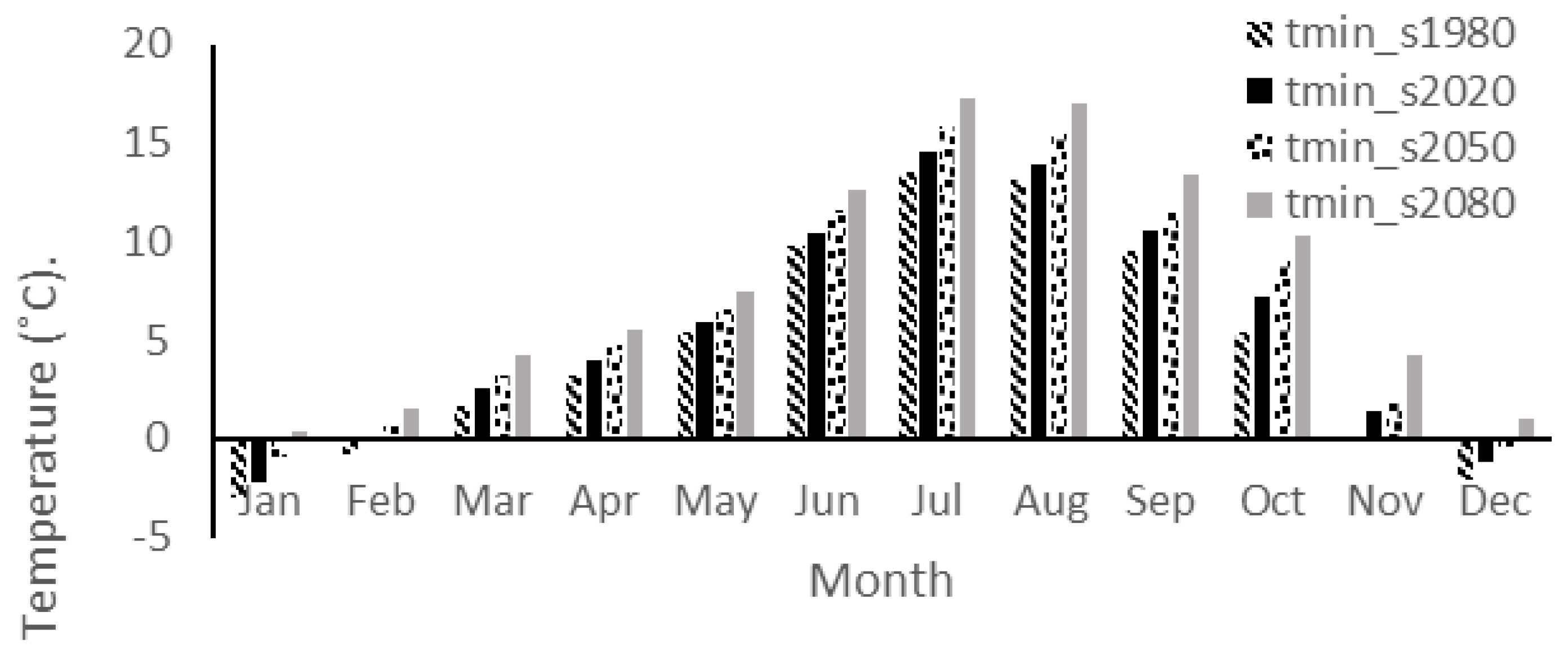
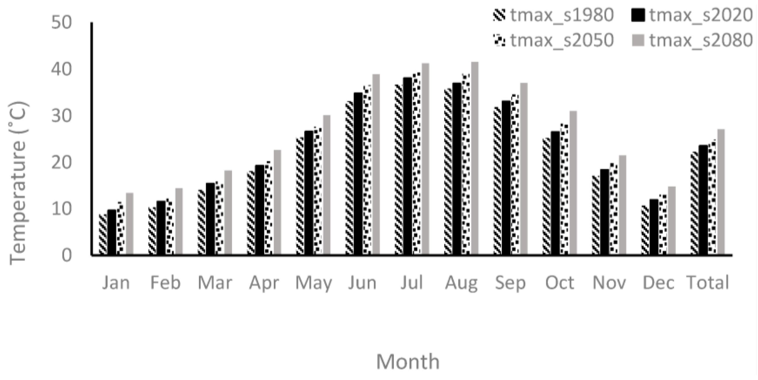
Crop production is the major agricultural activity in the Kermanshah township. This study has established that precipitation and temperature in the study area have been decreasing and increasing, respectively. In other words, under scenario A2, three time periods (2020, 2050, and 2080) were simulated. According to our simulated model, precipitation showed a decreasing trend, whereas temperature showed an increasing trend. This, in turn, negatively affects the sustainable production and management of water resources in the western part of Iran. The question is what impact this climate prediction has for the region. First, the findings of this study have great implications for devising climate change impact adaptation policies, as well as for managing and mitigating the impacts and reducing the vulnerabilities of local communities. This may come as an early warning to producers engaged in agricultural production. In this case, farmers must take adaptive measures to offset the negative impacts of climate variability. For example, a combination of strategies to adapt, such as proper timing of agricultural operations, crop diversification, the use of different crop varieties, changing planting dates, the increased use of water and soil conservation techniques, and diversifying from farm to non–farm activities, may be required. Although Iranian farmers are using certain coping strategies to mitigate the impact of climate variability, they need to take proactive measures in their adaptations to climate change. Currently, farmers use contour ridges as a strategy to maximize penetration and enhance moisture conservation. In this case, minimum tillage tends to conserve available water and thus improve germination rates and control pest and diseases. More research needs to be done on tillage practices in response to climate change impacts.

The result of this study can be used as an optimal model for land allocation in agriculture. A shortage of rainfall and decreased temperatures have implications for land allocation as well. For example, drought resistant crops with minimum water requirements are suggested. We also suggest that a better approach to continued research in this field, at the very least, should include both climate change and land allocation. Moreover, giving priority to the prediction of climate change and its role in agricultural and non-agricultural land allocation would greatly assist climate change research.

References

1. Iranian Statistic. 2016. Available online: http://www.amar.org.ir (accessed on 10 October 2016).
2. Faramarzi, M.; Abbaspour, K.C.; Schulin, R.; Yang, H. Model-ling blue and green water resources availability in Iran. Hydrol. Process. J. 2009, 23, 486–501. [Google Scholar] [CrossRef]
3. Pervez, M.S.; Henebry, G.M. Spatial and seasonal responses of precipitation in the Ganges and Brahmaputra river basins to ENSO and Indian Ocean dipole modes: Implications for flooding and drought. Nat. Hazards Earth Syst. Sci. 2014, 15, 147–162. [Google Scholar] [CrossRef]
4. Intergovernmental Panel on Climate Change (IPCC). Summary for Policy Makers. Climate Change 2007: The Physical Science Basis; Contribution of Working Group I to the Fourth Assessment Report; Cambridge University Press: Cambridge, UK, 2007. [Google Scholar]
5. Gordon, C.; Cooper, C.; Senior, C.A.; Banks, H.; Gregory, J.M.; Johns, T.C.; Mitchell, J.F.B.; Wood, R.A. The simulation of SST, sea ice extents and ocean heat transports in a version of the Hadley Centre coupled model without flux adjustments. Clim. Dyn. 2000, 16, 147–168. [Google Scholar] [CrossRef]
6. Ashrafi, K.; Shafiepour, M.; Ghasemi, L.; Najar Araabi, B. Prediction of Climate Change Induced Temperature Rise in Regional Scale Using Neural Network. Int. J. Environ. Res. 2012, 6, 677–688. [Google Scholar]
7. Kazemi Rad, L.; Mohammadi, H. Climate Change Assessment in Gilan province, Iran. Int. J. Agric. Crop Sci. 2015, 8, 86–93. [Google Scholar]
8. Tate, E.; Sutcliffe, J.; Conway, D.; Farquharson, F. Water balance of Lake Victoria: Update to 2000 and climate change modelling to 2100. Hydrol. Sci. J. 2004, 49, 562–574. [Google Scholar]
9. Wilby, R.L.; Dawson, C.W.; Barrow, E.M. SDSM: A Decision Support Tool for the Assessment of Regional Climate Change Impacts. J. Environ. Model. Softw. 2002, 17, 147–159. [Google Scholar] [CrossRef]
10. Bardossy, A. Downscaling from GCMs to local climate through stochastic linkages. J. Environ. Manag. 1997, 49, 7–17. [Google Scholar] [CrossRef]
11. Barrow, E.; Hulme, M.; Semenov, M.A. Effect of using different methods in construction of climate change scenarios: Examples from Europe. J. Clim. Res. 1996, 7, 195–211. [Google Scholar] [CrossRef]
12. Mearns, L.O.; Bogardi, I.; Giorgi, F.; Matyasovskey, I.; Paleski, M. Comparison of climate change scenarios generated from regional climate model experiments and statistical downscaling. J. Geophys. Res. 1999, 104, 6603–6621. [Google Scholar] [CrossRef]
13. Murphy, J. An evaluation of statistical and dynamical techniques for downscaling local climate. J. Clim. Chang. 1999, 12, 2256–2284. [Google Scholar] [CrossRef]
14. Sayari, N.; Mohammad, B.; Farid, A.; Alizadeh, A.; Hessami, M.R. Crop Water Consumption and Crop Yield Prediction under Climate Change Conditions at Northeast of Iran. In Proceedings of the 2011 International Conference on Environmental and Computer Science (IPCBEE), Singapore, 16–18 September 2011; IACSIT Press: Singapore, 2011; Volume 19, pp. 112–117. [Google Scholar]
15. Salon, S.; Cossarini, G.; Libralato, S.; Gao, X.; Solidoro, S.; Giorgi, F. Downscaling experiment for the vencie lagoon. I. validation of the present-day precipitation climatology. J. Clim. Res. 2008, 38, 31–41. [Google Scholar] [CrossRef]
16. Wilby, R.L.; Dawson, C.W. Using SDSM Version 3.1—A Decision Support Tool for the Assessment of Regional Climate Change Impacts; User Manual; Environment Agency of England and Wales: Nottingham, UK, 2004; p. 67. [Google Scholar]
17. Nury, A.H.; Alam, M.J.B. Performance Study of Global Circulation Model HADCM3 Using SDSM for Temperature and Rainfall in North-Eastern Bangladesh. J. Sci. Res. 2014, 6, 87–96. [Google Scholar] [CrossRef]
18. Johns, T.C.; Gregory, J.M.; Ingram, W.J.; Johnson, C.E.; Jones, A.; Lowe, J.A.; Mitchell, J.F.B.; Roberts, D.L.; Sexton, D.M.H.; Stevenson, D.S.; et al. Anthropogenic climate change for 1860 to 2100 simulated with the HadCM3 model under updated emissions scenarios. Clim. Dyn. 2003, 20, 583–612. [Google Scholar]
19. Taie Semiromi, M.; Koch, M.; Taie Semiromi, S. Prediction of Climate Change Impacts on Groundwater Storage by Analysis and Modeling of Hydrograph Recession Curves: Application to the Bar Watershed, Iran. Infect. Control Hosp. Epidemiol. 2014, 32, 809–817. [Google Scholar]
20. Jonathan, A.N. Using the output from global circulation models to predict changes in the distribution and abundance of cereal aphids in Canada: A mechanistic modeling approach. Glob. Chang. Biol. 2006, 12, 1634–1642. [Google Scholar]
21. Valizadeh, J.; Ziaei, S.M.; Mazloumzadeh, S.M. Assessing climate change impacts on wheat production (a case study). J. Saudi Soc. Agric. Sci. 2014, 13, 107–115. [Google Scholar] [CrossRef]
22. De Silva, C.S. Impacts of Climate Change on Water Resources in Sri Lanka. In Proceedings of the 32nd WEDC International Conference, Colombo, Sri Lanka, 13–17 November 2006; pp. 289–295.
23. Bekele, E.G.; Knapp, H.V. Watershed modeling to assessing impact of potential climate change on water supply availability. Water Resour. Manag. 2010, 24, 3299–3320. [Google Scholar] [CrossRef]
24. Koocheki, A.; Nassiri, M. Impacts of climate change and CO2 concentration on wheat yield in Iran and adaptation strategies. Iran. Field Crops Res. 2008, 6, 139–153. (In Persian) [Google Scholar]
25. Villegas, J.R.; Jarvis, A. Downscaling Global Circulation Model Outputs: The Delta Method Decision and Policy Analysis Working Paper. 2010. Available online: http://gisweb.ciat.cgiar.org/GCM (accessed on 22 November 2016).
26. Yang, Y.S.; Wang, L. Review of modeling tools for implementation of the EU Water Framework Directive in handling diffuse water pollution. Water Resour. Manag. 2010, 24, 1819–1843. [Google Scholar] [CrossRef] [Green Version]
Figure 1. Study area.
Sustainability 09 00146 g001
Figure 2. Calibration of monthly average minimum temperature at the Kermanshah synoptic station.
Sustainability 09 00146 g002
Figure 3. Validation of monthly average minimum temperature at the Kermanshah synoptic station.
Sustainability 09 00146 g003
Figure 4. Calibration of the monthly average maximum temperature at the Kermanshah synoptic station.
Sustainability 09 00146 g004
Figure 5. Validation of the monthly average maximum temperature at the Kermanshah synoptic station.
Sustainability 09 00146 g005
Figure 6. Calibration of the monthly average precipitation at the Kermanshah synoptic station.
Sustainability 09 00146 g006
Figure 7. Validation of the monthly average precipitation at the Kermanshah synoptic station.
Sustainability 09 00146 g007
Figure 8. Prediction of the monthly minimum temperature under the A2 scenario during different time periods at the Kermanshah synoptic station.
Sustainability 09 00146 g008
Figure 9. Prediction of the monthly maximum temperature under the A2 scenario during different time periods at the Kermanshah synoptic station.
Sustainability 09 00146 g009
Figure 10. Prediction of the monthly precipitation under the A2 scenario during different time periods at the Kermanshah synoptic station.
Sustainability 09 00146 g010