Government Subsidy for Remanufacturing or Carbon Tax Rebate: Which Is Better for Firms and a Low-Carbon Economy

Abstract

The government as a policy maker wishing to promote remanufacturing and proper disposal of hazardous old products which are harmful to environment has taken many actions, ranging from carbon regulation and financial incentives such as trade-in subsidy. However, carbon tax can result in loss of profit for firms to some degree, so the government has to give other subsidy to balance the profits and carbon emission. Thus, this article investigates two subsidy mechanisms: remanufacturing subsidy or tax rebate. The optimal pricing and production decision under these policies are examined. Our results show that carbon tax has a great impact on pricing strategies. Trade-in subsidy can encourage customers to replace their existing products with new and remanufactured products. Both remanufacture subsidy and tax rebate are beneficial to manufacturer and can further promote remanufacturing development.

1. Introduction

With the increasing concern of resources and environmental problems, energy conservation and carbon emission reduction have become a heated topic in the current social community. With the arrival of the low-carbon era, governments and enterprises are taking a series of measures to respond to the current circumstances. On the one hand, the government is taking measures such as carbon tax and constraint of carbon emission and so on to change the mode of production and operations for enterprises to mitigate carbon emissions. On the other hand, governments can provide subsidy for encouraging enterprises to make environment-friendly products and then advocate consumers to use them. In response to the changes in the government measures and the market, enterprises have to adjust their production plans and ensure their own profits. Recycling and then remanufacturing are beneficial to forming the cyclic economic mode of resources-products-used products-remanufactured products, fully making use of resources and protecting the ecological environment, which is the significant measure of realizing the low-carbon economic development.

Remanufacturing is a process to make the old machines with renewed vigor of life. It uses the old machinery and equipment as cores, and by the means of the special craft and technology to make a new product on the basis of the original product. The key process to remanufacturing is to recycle the used products as the resources available for remanufacturing. On the contrary, the persistent use and inappropriate disposal of some old products involves energy consumption and can cause environmental pollutions, such as used cars and waste household appliances. If the waste products can be recycled for remanufacturing, carbon emissions can fall dramatically. As a special mode of collection, trade-in not only takes back used products (otherwise known as cores) for remanufacturing but also brings many added benefits. Such practices have been widely observed. From an economic perspective, McConocha and Speh claim that recycling and then dismantling, renovation, and remanufacturing save cost, shorten the production cycle and bring new opportunities of development [1]. From a strategic perspective, remanufacturing with trade-ins can expand the scale of products sales and cultivate brand loyalty and at the same time reduce the competition in the second-hand market. From a perspective of environmental protection, remanufacturing with trade-ins reduces the waste of resources and energy consumption and increase environmental awareness of consumers. Through remanufacturing with trade-ins, there is a close correlation between recycling and sales. Trade-in consumers hand over old products to the recycling agents, recycling agents (usually the retailer or the manufacturer) provide rewards for consumers and sell their products to customers at a discount (usually the government provides subsidies). Subsequently, recycled products are disassembled or refurbished and remanufactured. In China, the government launched the trade-in program for home appliances in 2009, and initiated the program of trade-in for remanufactured automobile components in 2013.

Remanufacturing has a promising future, but it is developing slowly owing to the constraints imposed by the traditional consumption concepts and technological advancement, and thus the low payoff leads to the low initiative of enterprises. The subsidy is the most direct way for the government to encourage enterprises to remanufacture and attract the customers to purchase remanufactured products. To illustrate, in 2008, China’s “The Law of Boosting the Cyclic Economy” regulates remanufacturing, and in 2010, 11 Ministries and Commissions such as China’s National Development and Reform Commission issued collaboratively “Comments on Boosting the Remanufacturing Development”. The prior research has shown that the government subsidy can promote the remanufacturing development and conducive to manufacturers, remanufacturers, retailers and customers as well as other members in closed-loop supply chain [2,3].

Remanufacturing and trade-in programs are closely correlated to potential reduction in carbon emissions that are becoming a common concern shared by governments. As an effective and economical measure, carbon tax is also drawing much attention. Currently, Finland, The Netherlands and Sweden have formulated carbon tax system and achieved substantial results. Nonetheless, much research shows that carbon tax increases cost for enterprises to a greater extent and has negative effect on firms’ profit. A number of scholars have proposed a policy for the design of carbon tax system to minimize the negative impact. Against this backdrop, this article notes that the aim of collecting carbon tax from enterprises is to ensure low-carbon production and stimulate manufacturers to make more remanufactured products with carbon tax to reduce the cost of carbon emissions. However, as a result of the constraints imposed by the traditional consumption concepts and technological advancement, remanufacturing cannot enable enterprises to achieve more profits. Therefore, to reduce the negative impact of carbon tax and balance firms’ profit and carbon emission cost, the government has two neutral tax policies which transfer carbon tax from enterprises to low-carbon high-tech emerging industries (remanufacturing): government subsidy for remanufacturing and carbon tax rebate. This article aims to compare these two methods of transferring payments.

To develop a better understanding of exploring which policy is better for firms and low-carbon economy we address the following questions:

(1)

When the government introduces the carbon tax and the trade-in program, what is the optimal pricing and production strategy and in different government policies?

(2)

Can the firm be more profitable in the mode of government subsidy or carbon tax rebate compared to the scenario in which no government subsidy is provided?

(3)

Which mode of policy is appropriate for the environment and remanufacturing development?

The rest of this paper is organized as follows. After reviewing relevant literature in Section 2, we introduce two policy models in Section 3. Section 4 solves the equilibrium in these two models. Section 5 presents a comparison of equilibrium results, consumer surplus, social welfare, and environmental impact between the two modes. Additional numerical experiments are presented in Section 6, which is followed by the conclusion and implications in Section 7.

2. Literature Review

This paper builds upon four streams of research in the literature: remanufacturing, trade-in, carbon regulation and government subsidy.

Remanufacturing is considered as an essential link in the closed-loop supply chain, which has been investigated by researchers from different perspectives. An increasing mass of research has addressed remanufacturing strategies, such as acquisition of used products, cannibalization between new and remanufactured products and competition between OEM and IO. The original manufacturers are always confronted with the choice of whether to remanufacture. A number of manufacturers do not opt for remanufacturing if they consider that remanufacturing can cannibalize the high marginal profits of new products. However, when the original manufacturers are not involved in remanufacturing, professional remanufacturers emerge and that can hurt profits of the original manufacturers. Ferguson and Toktay assume that the original manufacturers are not involved in remanufacturing and there is no competition between the original manufacturers and remanufacturers. Thus, the original manufacturers may lose part of potential profits [4]. Now, the original manufacturers may prevent the competition from the third party by remanufacturing or first recycling used products. Ferrer and Swaminathan discuss the two-period, multi-phase or indefinite models of remanufacturing. On the one hand, the monopoly of the original manufacturers is considered, namely, the critical conditions necessary for making new and remanufactured products. On the other hand, the oligopolistic competition is also taken into account between the original manufacturers and remanufacturers [5]. Heese and Cattani analyze the remanufacturing profits in the original equipment manufacturer (OEM) competition on the basis of the Stahlberg model of double oligopolies [6]. The aforementioned studies have provided significant contributions for understanding remanufacturing. Bhattacharya and Savaskan compare three recycle modes, namely, manufacturers’, retailers’ and third parties’ recycle, and they find that retailer’s recycle is the best under some assumptions [7]. Gu examines manufacturers’, retailers’ and third parties’ recycle modes in terms of the optimal recycle cost and the profits of closed-loop supply chain members and shows that manufacturers’ recycle is desirable [8]. These studies compare which recycle channel is optimal under some conditions, whereas the reality is multiple channels coexist with competition and cooperation among them. For these reasons, Huang and Song study the manufacturers’ optimal pricing and recycle strategies when retailers and manufacturers recycle jointly [9]. Liu and Lei builds a competitive model of double channel recycling where the formal channel led by the recycle dealers with dismantling qualifications and the informal channel led by the recycle dealers without dismantling qualifications compete and depicts recycling disposal approaches and profit models of these two channels [10]. In brief, closed-loop supply chain members recycle on their own, or recycle jointly with other members, or collaborate with other supply chain members by contract, in accordance with their needs and understanding of markets. The former research regard recycle and sale as separate link and trade-in implies a strong connection between collection and sales and can reflect that recycling to promote sales, sales promote recycling.

However, trade-in practices have received limited attention. Zhu and Wang construct a two-stage model in a duopoly competition in which one enterprise is implementing trade-in while the other does not, and the result indicate that it is beneficial to adopt trade in which can bring competitive advantage in terms of market share and profits [11]. Li and Xu make a comparison between trade-in and leasing of a product with technology innovations, and state that trade-in protects the manufacturer against salvage value risk and allows the flexibility of offering the option at different innovation states separately [12]. Okada looks at the psychology and behavior of consumers involved in trade-in [13]. Zhang examines the impact of the government’s trade-in policy on the profits of enterprises and environment when there are strategic consumers [14]. Miao shows that the profit in the mode of the manufacturer’s recycle is greater than that in the mode of the retailer’s recycle in the trade-in program [15]. Ray considers the optimal trade-in rebate in the market of durable products and the pricing of products [16]. In this paper, we are also concerned with both trade-in and remanufacturing problems (the manufacturer involved in recycling and sale) to investigating pricing and production strategies. It has been shown that the manufacturer can gain part of subsidy from customers via the optimal recycle price in the government’s trade-in subsidy.

The literature discussed above concentrate on the corporate profit as the decision target, neglecting the realization of social targets like environment, energy resources and carbon emissions. Montgomery first proposed the concept of trade of carbon emissions [17]. Laffont and Tirole mainly consider the design of the market of carbon emissions [18]. The carbon tax has some negative impact on economy, which is determined by the cost of carbon tax. As such, most research focuses on the impact of carbon tax on the macro-economy in China. Benjaafar explores how carbon emissions influence the decision on purchase, production and inventory management of enterprises [19]. Chen et al. study varying models of corporate production strategies under the carbon constraint, and they show that the appropriate management of production and operation can achieve the significant reduction of carbon emissions at the relatively small economic cost [20]. Hua et al. investigate the changes of carbon trace of the enterprise’s inventory with carbon limitation in the carbon trade and construct the model of the optimal order quantity with the carbon constraint [21]. Some other studies also explore the optimal transportation strategies and the choice of suppliers with different constraints of carbon emissions such as carbon tax, carbon limitation and carbon trade. Based on the research above, this article examines manufacturing and remanufacturing with carbon regulations.

Actually, the government plays a pivotal role in development of remanufacturing and a large number of researchers have examined the closed-loop supply chain involving the government. Wang and Chen categorize the government policies and regulations related to recycling in China, and they note that trade-in can promote recycle of used products [22]. Ma and Zhao compare the two cases of consumers with or without government subsidy in the dual-channel closed-loop supply chains, and they notice that when the government subsidizes consumers, the profits of manufacturers, retailers and customers increase simultaneously [2]. Wang and Chang deploy systemic dynamics to examine the impact of different government subsidies, including initial subsidy, recycle subsidy, research and development subsidy and production subsidy on remanufacturing [23]. Mitra and Webster compare the cases when manufacturers or remanufacturers alone get subsidy or when they both get subsidy [24]. To sum up, there has been comprehensive research on the government subsidizing manufacturers, and most research claims that the government can make a positive contribution to promoting remanufacturing and guiding the consumption of remanufactured products.

In this article, we are concerned with remanufacturing related to both trade-in and carbon emission problems and propose different pricing and production strategies for different government policies. We provide a number of managerial insights for firms and policy makers.

3. Model Depiction and Assumptions

Based on the analyses above, governments encourage enterprises to engage in low-carbon production and urge manufacturers to make more remanufactured products under carbon tax. Due to the constraints imposed by the traditional consumption concepts and technological advancement, enterprises cannot obtain higher profits. Therefore, the government has two neutral tax policies which transfer carbon tax from enterprises to low-carbon high-tech emerging industries (remanufacturing). This article aims to compare these two methods of transferring payments. (1) The government provides enterprises with subsidy for each unit of remanufactured product; (2) The government offers the manufacturer remanufacturing tax rebate. The government takes varying measures to encourage enterprises to develop remanufacturing and reduce environmental pollutions, and these two models can help the government to realize the low-carbon economy.

3.1. Trade-In Policy and Consumer Behavior

This article is concerned with one monopoly manufacturer who makes new products with raw materials and collects old products through trade-in to make remanufactured products. The production cost of new products is $c_n$, whereas the production cost of remanufactured products is $c_r$, and the recycle price is $v$. The government provides subsidy $s_t$ for consumers who trade in. In the market, there are two types of customers: the first-time buyers (new customers) and the replacement customers (trade-in customers). The new buyers do not have the used product before purchasing the product, while the replacement consumers who have own used products either keep the existing product without buying any products or trade-in their existing product or simply purchase products without trade-in. However, those who simply purchase products without trade-in cannot obtain the recycle price and the trade-in subsidy. It is assumed that consumers are rational, and thus the replacement consumers who have own used products tend to purchase products through trade-in. Supposing all customers in the market number 1, there are $\alpha$ new consumers and $1-\alpha$ replacement consumers, where $0\le \alpha \le 1$ [25].

New customers and replacement customers make their purchase decisions based on their utilities associated with new and remanufactured products after observing the price determined by the firm. In practice, a product is labeled as “new” or “remanufactured”, and this labeling affects consumers’ perception of value. Thus, customers have different preferences to new and remanufactured products. As a result, pricing discrimination is adopted by the firm. It is assumed that the consumer willingness to pay for new products is $\theta$, while the consumer willingness to pay for remanufactured products lower at $t\theta$, $0\le t\le 1$ [9]. Given new products price $p_n$, remanufactured products price $p_r$, and recycle price $v$, the utility the new consumer obtains from buying new products is: $U_n^{\alpha }=\theta -p_n$; the utility the new consumer obtains from buying remanufactured products is: $U_r^{\alpha }=t\theta -p_r$. When $U_n^{\alpha }>U_r^{\alpha }$ and $U_n^{\alpha }>0$, the new consumer buys new products; otherwise, when $U_r^{\alpha }>0$, the new consumer buys remanufactured products. In terms of consumers with old products, their cognitive value of possessing old products is $\delta \theta$, $0<\delta <t$ [25]. Hence, a trade-in customer buy new product can get utility: $U_n^{1-\alpha }=\theta -p_n+v+s_t-\delta \theta$; a trade-in customer buy remanufactured product can get utility: $U_n^{1-\alpha }=t\theta -p_r+v+s_t-\delta \theta$. When $U_n^{1-\alpha }>U_r^{1-\alpha }$ and $U_n^{1-\alpha }>0$, the trade-in consumer replace with new products; otherwise, when $U_r^{1-\alpha }>0$, the trade-in consumer replace with a remanufactured products. If $\theta >p_n$, new customers would consider buying new products; if $t\theta >p_r$, consumers would consider buying remanufactured products. If $\theta >p_n$ and $t\theta >p_r$, then consumers buy the product that offers the most utility. Only if $(t\theta -p_r)-(\theta -p_n)>0\mathrm{and}t\theta -p_r>0$, can new customers buy remanufactured product. This means $p_n-p_r>(1-t)\theta$, and $\theta >\frac{p_r}{t}$, namely $\frac{p_n-p_r}{1-t}>\theta >\frac{p_r}{t}$, which implies $p_r\le t{p}_n$. Therefore, when the manufacturer adopts the strategy of a low price for remanufactured products ($p_r\le t{p}_n)$, the demand of new consumers for new products is $q_n^{\alpha }=\alpha (1-\frac{p_n-p_r}{1-t})$, while the demand of remanufactured products from new consumers is $q_r^{\alpha }=\alpha (\frac{p_n-p_r}{1-t}-\frac{p_r}{t})$. When the manufacturer adopts the strategy of a high price for remanufactured products ($p_r>t{p}_n$), $(t\theta -p_r)<(\theta -p_n)$, all new consumers turn to buy new products: $q_n^{\alpha }=\alpha (1-p_n)$; their demand for remanufactured products is 0. Likewise, in terms of replacement consumers if $\theta >p_n+v+s_t-\delta \theta$, consumers tend to purchase new products; if $t\theta >p_r+v+s_t-\delta \theta$, consumers tend to buy remanufactured products. If $\theta -p_n+v+s_t-\delta \theta >0$ and $t\theta -p_r+v+s_t-\delta \theta >0$, then consumers replace used products with new or remanufactured depending upon the utility they obtain according to the manufacturer’s pricing strategy. Only if $t\theta -p_r+v+s_t-\delta \theta -(\theta -p_n+v+s_t-\delta \theta )>0\mathrm{and}t\theta -p_r+v+s_t-\delta \theta >0$, will trade-in customers buy remanufactured products. This means $p_n-p_r>(1-t)\theta \mathrm{and}\theta >\frac{p_r-v-s_t}{t-\delta }$, which implies $(t-\delta )p_n-(1-\delta )p_r+(1-t)(v+s_t)>0$. For discussion, here it is defined that $\Delta =(t-\delta )p_n-(1-\delta )p_r+(1-t)(v+s_t)$. Two cases are considered: $\Delta \ge 0\mathrm{and}\Delta <0$. When $\Delta \ge 0$, trade-in customer would consider buying new product: $q_n^{1-\alpha }=(1-\alpha )(1-\frac{p_n-p_r}{1-t})$; trade-in customer would consider buying remanufactured product if $q_r^{1-\alpha }=(1-\alpha )(\frac{p_n-p_r}{1-t}-\frac{p_r-v-s_t}{t-\delta })=\frac{(t-\delta )p_n-(1-\delta )p_r+(1-t)(v+s_t)}{(t-\delta )(1-t)}$. When $\Delta <0$, consumers having old products replace them with new product: $q_n^{1-\alpha }=(1-\alpha )(1-\frac{p_r-v-s_t}{1-\delta })$, $q_r^{1-\alpha }=0$. This article aims to investigate the impact of the government boosting remanufacturing development. To simplify and highlight analyses, it is assumed that remanufacturing is not less 0; that is, the pricing strategy of enterprises towards new and remanufactured products satisfies the following conditions: $p_r\le t{p}_n$ and $\Delta =(t-\delta )p_n-(1-\delta )p_r+(1-t)(v+s_t)>0$. Hence, the demand of new consumers for new and remanufactured products is: $q_n^{\alpha }=\alpha (1-\frac{p_n-p_r}{1-t})$, $q_r^{\alpha }=\alpha (\frac{p_n-p_r}{1-t}-\frac{p_r}{t})$; the demand of replacement customers for new and remanufactured products is: $q_n^{1-\alpha }=(1-\alpha )(1-\frac{p_n-p_r}{1-t})$, $q_r^{1-\alpha }=(1-\alpha )(\frac{p_n-p_r}{1-t}-\frac{p_r-v-s_t}{t-\delta })$.

3.2. Carbon Emission

The carbon tax aims to urge enterprises to take measures to reduce emissions in terms of technology, operation, and absoluteness through internalizing the exterior in supply chains. When the cost of carbon tax covers the profits of production, enterprises have to reduce emissions absolutely, namely to stop making products of enormous pollution, to satisfy the requirement of emission reduction. In order to control carbon emissions, the government usually imposes tax regulations on enterprises. Currently, two major modes of carbon regulations are widely used: carbon tax and carbon trade. This article concerns the mode of carbon tax. For instance, Canada imposes carbon tax on the consumption of coal, petroleum and gasoline. We define the rate of carbon tax levied by the government is $c$, as the additional linear cost associated with carbon emissions. Usually, the emission of making remanufactured products is less than that of making new products, because less material and energy is consumed in the manufacturing process. It is assumed that the carbon emission of producing the unit new product is $e_n$($e_n>0$), while the carbon emission of producing the unit remanufactured product is $e_r$($e_r>0$) and $e_n>e_r$. Therefore, the manufacturer’s cost of carbon emission is $CE=e_{n}c$($q_n^{\alpha }+q_n^{1-\alpha }$) + $e_{r}c$($q_r^{\alpha }+q_r^{1-\alpha }$). It can be seen from this equation that the increasing demand for the manufacturer’s products means greater carbon emission and higher cost. However, the higher demand for products means the greater profits of the manufacturer. Thus, it is important for the manufacturer to seek the optimal combination between profit and carbon emission. The impetus of the combination is the optimal production decision on manufacturing and remanufacturing. As the policy maker of carbon tax, the government has an opportunity to moderate carbon tax to facilitate or force enterprises to adjust their production.

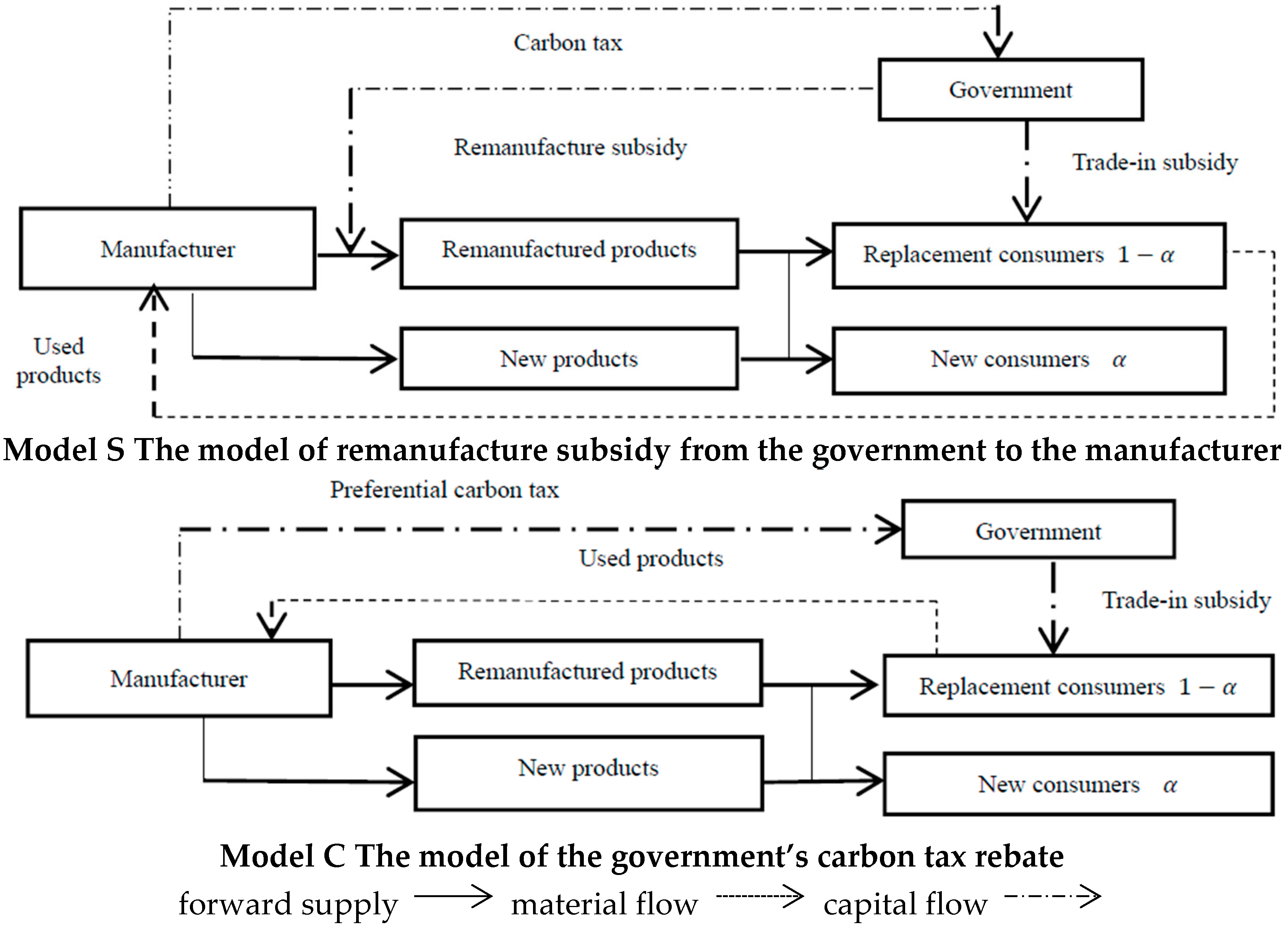
3.3. The CLSC Models with Trade-In under Different Policies

In Model S, the government subsidizes remanufacturing, and remanufacture subsidy is a common method of incentive from the government. In the mode of remanufacture subsidy from the government, the government subsidizes $s_r$ for enterprises making the unit remanufactured product [26]. In Model C, the government imposes varying tax standards for carbon emission from new and remanufactured products. The tax imposed on the unit carbon emission from new products is $c$, whereas the tax imposed on the unit carbon emission from remanufactured products is $\rho c$. Since carbon emission from remanufactured product is less than that from new products, it is assumed that $\rho <1$ to encourage remanufacturing to achieve the goal of sustainable development (see Figure 1).

To explain the model clearly, the symbols of variables are summarized in

Table 1. Variable list.

Parameters	Definitions
$p_n$/$p_r$	Selling price of new products and remanufactured products
$c_n$/$c_r$	Unit cost of new products and remanufactured products
$v$	Recycle price of used products
$s_t$	Trade-in subsidy
$\alpha$	The proportion of new consumers is $0<\alpha <1$, so the proportion of replacement consumers is $1-\alpha$
$q_n^k$/$q_r^k$	The demand for of products and remanufactured products from new consumers or repeat consumers (k = $\alpha ,1-\alpha$)
$\theta$	Willingness to pay of new products
t$\theta$	Willingness to pay of remanufactured products
$\delta \theta$	Consumers’ cognitive value for possessing used products
$e_n/e_r$	Unit carbon emission from new products and remanufactured products
$c$	Tax of unit carbon emission from new and remanufactured products in the mode of remanufacture subsidy
$s_r$	Subsidy for the unit remanufactured product in the mode of remanufacture subsidy
$\rho c$	Tax of unit carbon emission from remanufactured products in the mode of tax rebate
${\mathrm{\Pi }}_M$	Manufacturer’s profits

and some relevant assumptions are expounded.

4. Model Formulation and Solution

In this section, the manufacturer’s optimal pricing strategy and decisions on manufacturing and remanufacturing in different government policies are examined. The manufacturers in closed-loop supply chains aim to maximize their profits through determining the optimal $p_n^{*}$ and $p_r^{*}$. Here, ${\mathrm{\Pi }}_M^X$(${\mathrm{\Pi }}_M^{X*}$) indicates the manufacturer’s profit (the maximal profits of manufacturers). $X=S,C$, where $S$ and $C$ are the superscripts of the models in different government policies implemented. Below, to differentiate each relevant value in the two different models, the relevant symbols in Model $S$ are marked with the superscript of $S$, while the relevant symbols in Model $C$ are marked with the superscript of $C$.

4.1. Model S—Remanufacture Subsidy from the Government to the Manufacturer

In this model, the government provides unit subsidy to remanufacture to reduce production cost and then encourage enterprises remanufacture. It is assumed that there are both new and remanufactured products in the current market. The old products owned by consumers made previously can be collected through trade-in in this period, and for remanufacturing in the next period. In this article, only one single period is considered. It is assumed that the unit salvage of the old products is a constant $b$ [25]. To maximize the total profit from both new and remanufactured products, the manufacturer solves the following optimization problem:

$${\mathrm{Max}\mathrm{\Pi }}_M^S=(p_n-c_n-c{e}_n)(q_n^{\alpha }+q_n^{1-\alpha })+(p_r-c_r+s_r-c{e}_r)(q_r^{\alpha }+q_r^{1-\alpha })-(v-b)(q_n^{1-\alpha }+q_r^{1-\alpha })$$

(1)

Proposition 1.

In Model S, when $c_r+c{e}_r\le t(c_n+c{e}_n)+s_r$ and $(t-\delta )(c_n+c{e}_n)-(1-\delta )(c_r+c{e}_r)+(1-t)(b+s_t)+(1-\delta )s_r\ge 0$ , the combination of the manufacturer’s optimal pricing strategies is:

$$p_n^{S*}=\frac{1+c_n+c{e}_n}{2};p_r^{s*}=\frac{t+c_r+c{e}_r-s_r}{2};v^{s*}=\frac{b+\delta -s_t}{2}$$

According to Proposition 1 above: (1) The sale price of new products is dependent on the cost structure and carbon tax. The price increases with the rise of production cost $c_n$ and carbon tax rate $c$; (2) The price of remanufactured products mainly depends on consumer willingness to pay $t$, remanufacturing cost $c_r$, carbon tax rate $c$, and government remanufacturing subsidy $s_r$. The price of remanufactured products increases with a rise in the production cost $c_r$ and carbon tax $c$. The price of remanufactured products increase with a rise in $t$, in particular with respect to the green consumers, who are willing to spend more on remanufactured products in consideration of environmental protection. Hence, it is unnecessary for enterprises to adopt the strategy of a low price for capturing price-sensitive consumers. With the remanufacture subsidy from the government, production costs are reduced and then the prices are lower. When the government subsidizes remanufacturing, enterprises tend to share part of the subsidy with consumers to attract them and increase their own sales; (3) The recycle price (the price at which used products are bought from consumers) is affected by the salvage value of old product $b$, consumers’ cognitive value of old products $\delta$, and the government’s trade-in subsidy $s_t$. If the salvage value of old products $b$ is significant for the firm, and the perceived economic value increases, enterprises are willing to raise the recycling price. Additionally, if consumers’ cognitive value of old products $\delta$ is big and consumers are more willing to keep using old products, then the desire to trade-in is lower. Thus, it is important for enterprises to raise recycle price to stimulate consumers to replacement products. In addition, from the Equation $v^{s*}=(b+\delta -s_t)/2$, it is clear that when $b+\delta >s_t$, the recycle price is negative. When the salvage value $\mathrm{b}$ of old products is very small or the value $\delta$ of using old products is low for consumers or both of them are low, consumers are supposed to pay for enterprises that recycle in the mode of government subsidy. It is likely that the government forces enterprises to dispose some old products with tremendous pollution, and the negative recycle price is actually the subsidy for enterprises to recycle and treat some used products. When the amount of government subsidy is enormous, enterprises tend to extract part of subsidy from consumers through the recycle price. Thus, it is necessary for the government to set the optimal subsidy; (4) The impact of carbon tax on the pricing of new products is greater than that of remanufactured products because remanufactured products are generally associated with less carbon emission than new products due to the energy and material savings.

Proposition 2.

The demand of new products and remanufactured products under the optimal pricing policies can be derived as follows:

The demand from new consumers for new products is:

$$q_n^{\alpha S*}=\alpha (\frac{1}{2}-\frac{c_n+c{e}_n-c_r-c{e}_r+s_r}{2(1-t)})$$

(2)

The demand from new consumers for remanufactured products is:

$$q_r^{\alpha S*}=\alpha \frac{t{c}_n+tc{e}_n-c_r-c{e}_r+s_r}{2t(1-t)}$$

(3)

The demand from replacement consumers for new products is:

$$q_n^{(1-\alpha )S*}=(1-\alpha )(\frac{1}{2}-\frac{c_n+c{e}_n-c_r-c{e}_r+s_r}{2(1-t)})$$

(4)

The demand from replacement consumers for remanufactured products is:

$$q_r^{(1-\alpha )S*}=(1-\alpha )\frac{(t-\delta )(c_n+c{e}_n)-(1-\delta )(c_r+c{e}_r)+(1-t)(b+s_t)+(1-\delta )s_r}{2(t-\delta )(1-t)}$$

(5)

The quantity of recycling of old products is the quantity demanded by consumers who trade in:

$$q_v^s=q_n^{(1-\alpha )S*}+q_r^{(1-\alpha )S*}=(1-\alpha )\frac{t+b+s_t+s_r-(c_r+c{e}_r)-\delta }{2(t-\delta )}.$$

According to the above proposition, the manufacture’s production decisions are dependent on the cost structure of new and remanufactured products, and carbon tax, the salvage value perceived by firm and consumers, and the subsidy from government. (1) With a rise in the production cost of new products, the output of new products declines while the output of remanufactured products steps up. With the rising production cost of remanufactured products, the output of new products increases while the output of remanufactured products drops; (2) The subsidy from the government does not have any impact on the new consumer, but it can encourage trade-in consumers to buy remanufactured ones; (3) The remanufacture subsidy to the enterprises from the government reduces the output of new products, playing a positive role in promoting remanufacturing development; (4) With trade-ins, the demand in replacement market is also affected by the salvage value of old products perceived by firms and customers; (5) When remanufacturing has advantage in carbon emissions, namely $e_r\le t{e}_n$ and $(1-\delta )e_r<(t-\delta )e_n$, carbon tax has a reverse effect on the output of new products while boosting the production of remanufactured products. Conversely, the output of both new and remanufactured products declines with the rising carbon tax $c$; (6) The quantity of products recycled is negatively associated with remanufacturing cost. The greater the remanufacturing cost, the lower is the willingness of enterprises to remanufacture. Enterprises are not willing to recycle old products. The recycling quantity of old products is positively associated with the trade-in subsidy of the government (see

Table 2. Monotonicity of product quantity on $c_n$, $c_r$, $s_t$ and $s_r$.

Variables	${\mathit{q}}_{\mathit{n}}^{\mathit{\alpha }\mathit{S}*}$	${\mathit{q}}_{\mathit{r}}^{\mathit{\alpha }\mathit{S}*}$	${\mathit{q}}_{\mathit{n}}^{(\mathbf{1}-\mathit{\alpha })\mathit{S}*}$	${\mathit{q}}_{\mathit{r}}^{(\mathbf{1}-\mathit{\alpha })\mathit{S}*}$
$c_n/c_r$ ↗	↘/↗	↗/↘	↘/↗	↗/↘
$s_t$ ↗	→	→	→	↗
$s_r$ ↗	↘	↗	↘	↗
$c$ ↗	↘	↗	↘	↗

).

Now, the manufacturers’ optimal profits are:

$${\mathrm{\Pi }}_M^{S*}=(p_n^{S*}-c_n-c{e}_n)(q_n^{\alpha S*}+q_n^{(1-\alpha )S*})+(p_r-c_r-c{e}_r+s_r)(q_r^{\alpha S*}+q_r^{(1-\alpha )S*})-(v^{s*}-b)(q_n^{(1-\alpha )S*}+q_r^{(1-\alpha )S*})$$

4.2. Model C—Tax Rebate for Remanufacturing from the Government

In this model, the government launches carbon rebate for remanufacturing to encourage enterprises to remanufacture. In this mode, the unit tax of carbon emission for producing new products is $c$, while the unit tax of carbon emission for producing remanufactured products is $\rho c$. To maximize the total profit from both the new and the remanufactured products, the manufacturer solves the following optimization problem:

$${\mathrm{Max}\mathrm{\Pi }}_M^C=(p_n-c_n-c{e}_n)(q_n^{\alpha }+q_n^{1-\alpha })+(p_r-c_r-\rho c{e}_r)(q_r^{\alpha }+q_r^{1-\alpha })-(v-b)(q_n^{1-\alpha }+q_r^{1-\alpha })$$

(6)

Proposition 3.

In Model C, when $c_r+\rho c{e}_r\le t(c_n+c{e}_n)$ and $(t-\delta )(c_n+c{e}_n)-(1-\delta )(c_r+\rho c{e}_r)+(1-t)(b+s_t)\ge 0$ , the combination of the manufacturer’s optimal pricing strategies is:

$$p_n^{C*}=\frac{1+c_n+c{e}_n}{2};p_r^{C*}=\frac{t+c_r+\rho c{e}_r}{2};v^{C*}=\frac{b+\delta -s_t}{2}$$

From Proposition 3, it has been shown that the manufacturer’s combination of the optimal pricing strategies in Model C is similar to that in Model S. (1) The price of new and remanufactured products depends on cost structure, carbon tax, and consumer willingness to pay. Both new and remanufactured product’s sale price increases with a rise in the production cost and carbon tax. The price of remanufactured products increases with a rise of consumer willingness to pay; (2) In the mode of tax rebate, the impact of carbon tax on the pricing of new products is greater than that of remanufactured products, due to the fact that carbon emission from making new products is more than that from making remanufactured products and the tax of remanufactured products is lower than that of new products; (3) The recycle price is influenced by the salvage value of old products, consumers’ cognitive value of existing products, and the government’s trade-in subsidy. Similar to Model S, when the salvage value of old products is extremely low or consumers’ cognitive value of old products is very low or government subsidy is enormous, the recycle price of enterprises can be negative.

Proposition 4.

The demand for new and remanufactured products under optimal pricing policies can be derived as follows:

The demand from new consumers for new products is:

$$q_n^{\alpha C*}=\alpha (\frac{1}{2}-\frac{c_n+c{e}_n-c_r-\rho c{e}_r}{2(1-t)})$$

(7)

The demand from new consumers for remanufactured products is:

$$q_r^{\alpha C*}=\alpha \frac{t{c}_n+tc{e}_n-c_r-\rho c{e}_r}{2t(1-t)}$$

(8)

The demand from replacement customers for new products is:

$$q_n^{(1-\alpha )C*}=(1-\alpha )(\frac{1}{2}-\frac{c_n+c{e}_n-c_r-\rho c{e}_r}{2(1-t)})$$

(9)

The demand from replacement customers for remanufactured products is:

$$q_r^{(1-\alpha )C*}=(1-\alpha )\frac{(t-\delta )(c_n+c{e}_n)-(1-\delta )(c_r+\rho c{e}_r)+(1-t)(b+s_t)}{2(t-r)(1-t)}$$

(10)

The quantity of recycled old products is the quantity demanded by consumers who trade in:

$$q_v^C=q_n^{(1-\alpha )C*}+q_r^{(1-\alpha )C*}=(1-\alpha )\frac{t+b+s_t-(c_r+\rho c{e}_r)-\delta }{2(t-\delta )}$$

According to the above proposition, the manufacture’s production decisions depend upon the cost structure of new and remanufactured products, and carbon tax, the salvage value perceived by firm and consumers, and the trade-in subsidy from government. (1) With a rise in the production cost of new products, the output of new products declines while the output of remanufactured products goes up. With a rise in the production cost of remanufactured products, the output of new products increases while the output of remanufactured products goes down; (2) With a rise in carbon tax $c$ of new products, the output of new products drops, while the output of remanufactured products increases. With a rise in carbon tax rebate, namely lower $\rho$ of remanufactured products, the advantage to remanufacturing is strengthened, and the output of remanufactured products increases; (3) The trade-in subsidy from the government does not have any influence on the new consumer, while it can affect the trade-in consumers’ decision; (4) The recycling quantity of old products is negatively associated with remanufacturing cost. A higher remanufacturing cost means lower willingness of enterprises to remanufacture. Enterprises are not willing to recycle old products. The recycling quantity of old products is positively associated with the trade-in subsidy of the government (see

Table 3. Monotonicity of product quantity on $c_n$, $c_r$, $s_t$, $c$ and $\rho$.

Variables	${\mathit{q}}_{\mathit{n}}^{\mathit{\alpha }\mathit{S}*}$	${\mathit{q}}_{\mathit{r}}^{\mathit{\alpha }\mathit{S}*}$	${\mathit{q}}_{\mathit{n}}^{(\mathbf{1}-\mathit{\alpha })\mathit{S}*}$	${\mathit{q}}_{\mathit{r}}^{(1-\mathit{\alpha })\mathit{S}*}$
$c_n/c_r$ ↗	↘/↗	↗/↘	↘/↗	↗/↘
$s_t$ ↗	→	→	→	↗
$c$↗	↘	↗	↘	↗
$\rho$↗	↗	↘	↗	↘

).

Now, the manufacturers’ optimal profits are:

$${\mathrm{\Pi }}_M^{C*}=(p_n^{C*}-c_n-c{e}_n)(q_n^{\alpha C*}+q_n^{(1-\alpha )C*})+(p_r-c_r-\rho c{e}_r)(q_r^{\alpha C*}+q_r^{(1-\alpha )C*})-(v^{s*}-b)(q_n^{(1-\alpha )C*}+q_r^{(1-\alpha )C*})$$

(11)

5. Comparisons of Different Models

The discussions above involve manufacturers’ optimal pricing decisions in different models and a series of relevant indexes are derived. The analyses of which mode of subsidy can reduce the negative effect of carbon tax to manufacture’s profit and facilitate the government to boost the remanufacturing development are presented as follows.

To better explain the validity of government policy, a benchmark model is introduced here: the government does not provide remanufacture subsidy for manufacturers and does not launch tax rebate. Below, the case is marked with the superscript $N$. Therefore, without government remanufacture subsidy or tax rebate, the manufacturer’s profits are: ${\mathrm{Max}\mathrm{\Pi }}_M^N=(p_n-c_n-c{e}_n)(q_n^{\alpha }+q_n^{1-\alpha })+(p_r-c_r-c{e}_r)(q_r^{\alpha }+q_r^{1-\alpha })-(v-b)(q_n^{1-\alpha }+q_r^{1-\alpha })$.

In Model N, when $c_r+c{e}_r\le t(c_n+c{e}_n)$ and $(t-\delta )(c_n+c{e}_n)-(1-\delta )(c_r+c{e}_r)+(1-t)(b+s_t)\ge 0$, the optimal decision of manufacturers’ price is: $p_n^{C*}=\frac{1+c_n+c{e}_n}{2}$; $p_r^{C*}=\frac{t+c_r+c{e}_r}{2}$; $v^{C*}=\frac{b+\delta -s_t}{2}$. Hence, the maximal demand for new and remanufactured products is: $q_n^{\alpha N*}=\alpha (\frac{1}{2}-\frac{c_n+c{e}_n-c_r-c{e}_r}{2(1-t)}$); $q_r^{\alpha N*}=\alpha \frac{t{c}_n+tc{e}_n-c_r-c{e}_r}{2t(1-t)}$; $q_n^{(1-\alpha )N*}=(1-\alpha )(\frac{1}{2}-\frac{c_n+c{e}_n-c_r-c{e}_r}{2(1-t)})$; $q_r^{(1-\alpha )N*}=(1-\alpha )\frac{(t-\delta )(c_n+c{e}_n)-(1-\delta )(c_r+c{e}_r)+(1-t)(b+s_t)}{2(t-r)(1-t)}$.

The recycling quantity of used products is: $q_v^N=q_n^{(1-\alpha )N*}+q_r^{(1-\alpha )N*}=(1-\alpha )\frac{t+b+s_t-(c_r+c{e}_r)-\delta }{2(t-\delta )}$.

Therefore, the manufacturer’s optimal profits are: ${\mathrm{\Pi }}_M^{N*}=(p_n^{N*}-c_n-c{e}_n)(q_n^{\alpha N*}+q_n^{(1-\alpha )N*})+(p_r^{N*}-c_r-c{e}_r)(q_r^{\alpha N*}+q_r^{(1-\alpha )N*})-(v^{N*}-b)(q_n^{(1-\alpha )N*}+q_r^{(1-\alpha )N*})$.

Below are the comparisons made from equilibrium decisions and profits, environmental impact, consumer surplus and social welfare.

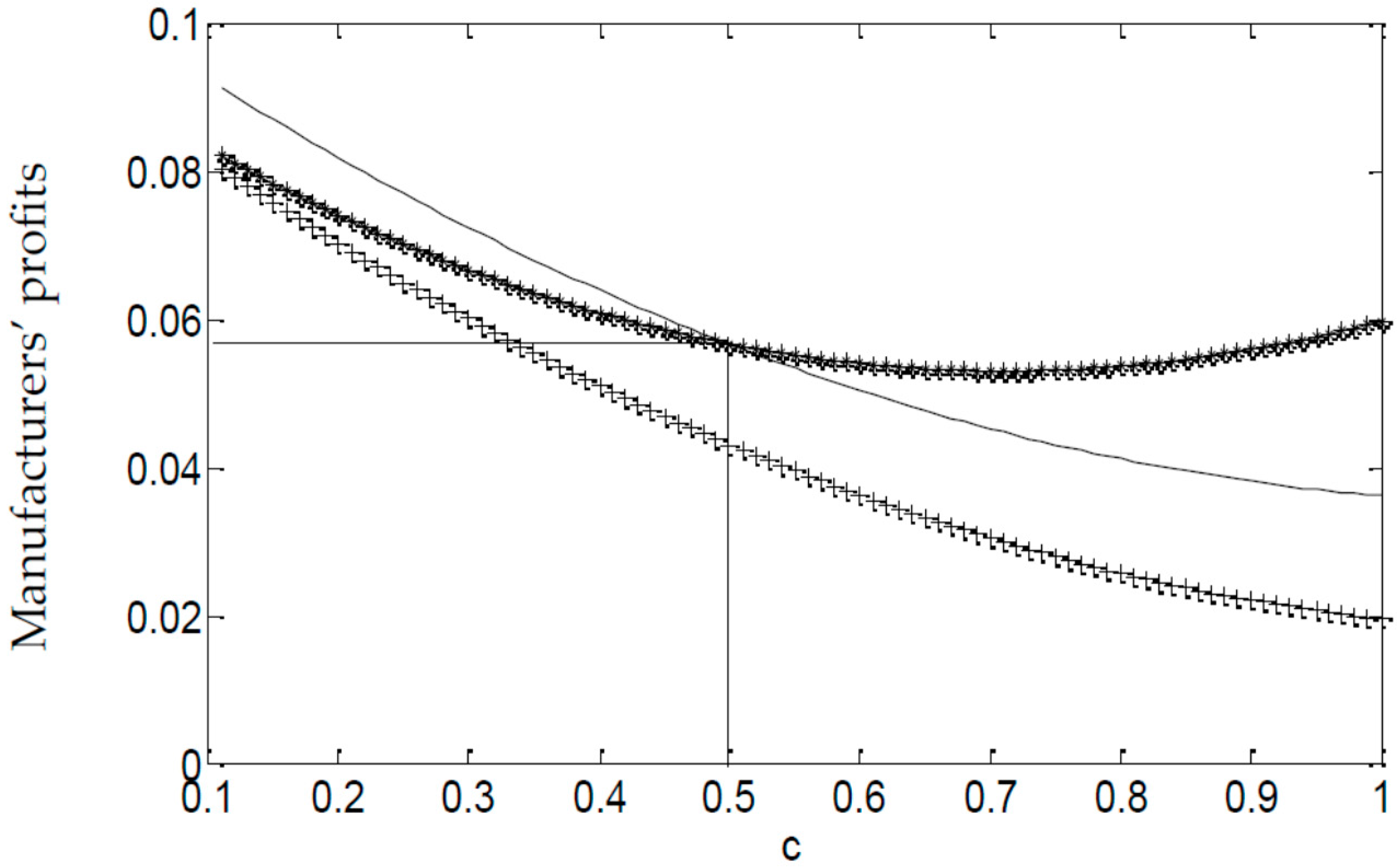
5.1. Comparison of Equilibrium Decisions and Profits

Observation 1.

The prices of new products in three models are the same: $p_n^{N*}=p_n^{S*}=p_n^{C*}$.

The price of making new products is only associated with their production cost and the rate of carbon tax. In the three models, the production cost of new products and the standard of carbon tax do not change, and thus their prices are fixed.

Observation 2.

The prices of remanufactured products in three models are: when $(1-\rho )c{e}_r\ge s_r$, $p_r^{N*}\ge p_r^{S*}\ge p_r^{C*}$. When $(1-\rho )c{e}_r<s_r$, $p_r^{N*}\ge p_r^{C*}\ge p_r^{S*}$.

The price of remanufactured products depends on remanufacturing cost, consumer willingness to pay, carbon tax and the relevant government policies. If the production cost and consumer willingness to pay do not change, the selling price of remanufactured products is highest in case without government subsidy. When the government subsidizes remanufacturing, the enterprise has the cost advantage in producing, the enterprise can sell at a low price and achieve greater sales volume and thus gain more profits. When the government provides the enterprise with remanufacture subsidy $s_r$, the price $\frac{s_r}{2}$ of remanufactured products drops, suggesting that the enterprise shares part of the government subsidy with the consumer.

Proof. 

$p_r^{N*}-p_r^{S*}=\frac{t+c_r+\mathrm{c}{e}_r}{2}-\frac{t+c_r+\mathrm{c}{e}_r-s_r}{2}=\frac{s_r}{2}>0$.

When the government introduces the tax rebate to enterprises remanufacturing, the remanufacturing cost of the carbon emission decreases compared with the case without subsidy. Thus, enterprises are able to attract more consumers through low prices. The tax rebate from the government is $(1-\rho )c{e}_r$, and the price of remanufactured products falls $\frac{(1-\rho )c{e}_r}{2}$.

Proof. 

$p_r^{N*}-p_r^{C*}=\frac{t+c_r+\mathrm{c}{e}_r}{2}-\frac{t+c_r+\mathsf{\rho }c{e}_r}{2}=\frac{(1-\rho )c{e}_r}{2}>0$.

When the unit subsidy of remanufacturing from the government to the enterprise is less than the unit carbon tax rebate of remanufactured products, $p_r^{S*}\ge p_r^{C*}$; otherwise, $p_r^{S*}\le p_r^{C*}$.

Proof. 

$p_r^{S*}-p_r^{C*}=\frac{t+c_r+\mathrm{c}{e}_r-s_r}{2}-\frac{t+c_r+c_0{e}_r}{2}=\frac{\mathrm{c}{e}_r-s_r-c_0{e}_r}{2}=\frac{(1-\rho )c{e}_r-s_r}{2}$.

Observation 3.

The recycle price for used products in the three models is the same: $v^{N*}=v^{S*}=v^{C*}$.

The recycle price of old products is associated with the salvage value ($b)$ of old products, consumers’ cognitive value $(\delta )$ of existing product, and the government’s trade-in subsidy $(s_t)$. $b$, $\delta$, and $s_t$ do not change in the three models, and thus their recycle price is the same.

Observation 4.

The new consumer’s and placement consumer’s demand for new and remanufactured products in the three models satisfies: when $(1-\rho )c{e}_r\ge s_r$, $q_n^{\alpha N*}\ge q_n^{\alpha S*}\ge q_n^{\alpha C*}$, $q_r^{\alpha C*}\ge q_r^{\alpha S*}\ge q_r^{\alpha N*}$ , $q_n^{(1-\alpha )N*}\ge q_n^{(1-\alpha )S*}\ge q_n^{(1-\alpha )C*}$; $q_r^{(1-\alpha )C*}\ge q_r^{(1-\alpha )S*}\ge q_r^{(1-\alpha )N*}$.

When $(1-\rho )c{e}_r<s_r$, $q_n^{\alpha N*}\ge q_n^{\alpha C*}\ge q_n^{\alpha S*},q_r^{\alpha S*}\ge q_r^{\alpha C*}\ge q_r^{\alpha N*}$, $q_n^{(1-\alpha )N*}\ge q_n^{(1-\alpha )C*}\ge q_n^{(1-\alpha )S*}$, $q_r^{(1-\alpha )S*}\ge q_r^{(1-\alpha )C*}\ge q_r^{(1-\alpha )N*}$.

Proof. 

$q_n^{\alpha N*}-q_n^{\alpha C*}=\alpha (\frac{1}{2}-\frac{c_n+c{e}_n-c_r-\mathrm{c}{e}_r}{2(1-t)})-\alpha (\frac{1}{2}-\frac{c_n+c{e}_n-c_r-\rho c{e}_r}{2(1-t)})=\alpha \frac{(1-\rho )c{e}_r}{2(1-t)}>0$ $q_n^{\alpha N*}-q_n^{\alpha S*}=\alpha (\frac{1}{2}-\frac{c_n+c{e}_n-c_r-\mathrm{c}{e}_r}{2(1-t)})-\alpha (\frac{1}{2}-\frac{c_n+c{e}_n-c_r-c{e}_r+s_r}{2(1-t)})=\alpha \frac{s_r}{2(1-t)}>0$ $q_n^{\alpha C*}-q_n^{\alpha S*}=\alpha (\frac{1}{2}-\frac{c_n+c{e}_n-c_r-\rho c{e}_r}{2(1-t)})-\alpha (\frac{1}{2}-\frac{c_n+c{e}_n-c_r-c{e}_r+s_r}{2(1-t)})=\alpha \frac{s_r-(1-\rho )c{e}_r}{2(1-t)}$ Therefore, when $(\mathrm{c}-c_0)e_r\ge s_r$, $q_n^{\alpha C*}-q_n^{\alpha S*}<0$, when $(\mathrm{c}-c_0)e_r<s_r$, $q_n^{\alpha C*}-q_n^{\alpha S*}>0$,

$$q_r^{\alpha N*}-q_r^{\alpha C*}=\alpha \frac{t{c}_n+tc{e}_n-c_r-\mathrm{c}{e}_r}{2t(1-t)}-\alpha \frac{t{c}_n+tc{e}_n-c_r-\rho c{e}_r}{2t(1-t)}=-(\alpha \frac{(1-\rho )c{e}_r}{2(1-t)})<0$$

$$q_r^{\alpha N*}-q_r^{\alpha S*}=\alpha \frac{t{c}_n+tc{e}_n-c_r-\mathrm{c}{e}_r}{2t(1-t)}-\alpha \frac{t{c}_n+tc{e}_n-c_r-c{e}_r+s_r}{2t(1-t)}=-\left(\alpha \frac{s_r}{2(1-t)}\right)<0$$

$$q_r^{\alpha C*}-q_r^{\alpha S*}=\alpha \frac{t{c}_n+tc{e}_n-c_r-\rho c{e}_r}{2t(1-t)}-\alpha \frac{t{c}_n+tc{e}_n-c_r-c{e}_r+s_r}{2t(1-t)}=-(\alpha \frac{s_r-(1-\rho )c{e}_r}{2(1-t)})$$

Therefore, when $(1-\rho )c{e}_r\ge s_r$, $q_r^{\alpha C*}-q_r^{\alpha S*}>0$, when $(1-\rho )c{e}_r<s_r$, $q_r^{\alpha C*}-q_r^{\alpha S*}<0$.

Likewise, the sales of the replacement consumers can be derived.

The recycling quantity of old products satisfies: when $(1-\rho )c{e}_r\ge s_r$, $q_v^C>q_v^S>q_v^N$, when $(1-\rho )c{e}_r<s_r$, $q_v^S>q_v^C>q_v^N$.

The proofs above show that the government’s remanufacture subsidy and tax rebate reduce the demand for new products and increase the demand for remanufactured products. The more is the subsidy from the government, the more is the demand for remanufactured products.

Observation 5.

The manufacturer’s profit in three models are: when $(1-\rho )c{e}_r\ge s_r$, ${\Pi }_M^{C*}\ge {\Pi }_M^{S*}\ge {\Pi }_M^{N*}$ ; when $(1-\rho )c{e}_r<s_r$ , ${\Pi }_M^{S*}\ge {\Pi }_M^{C*}\ge {\Pi }_M^{N*}$.

When the government provides remanufacture subsidy and tax rebate for enterprises, their profits tend to be greater than the case without any subsidy or benefit. When amount of the tax rebate is greater than that of remanufacture subsidy, the tax rebate is more favorable for enterprises. Conversely, enterprises hope that the government provides remanufacture subsidy.

The proof can be seen in the Appendix A.

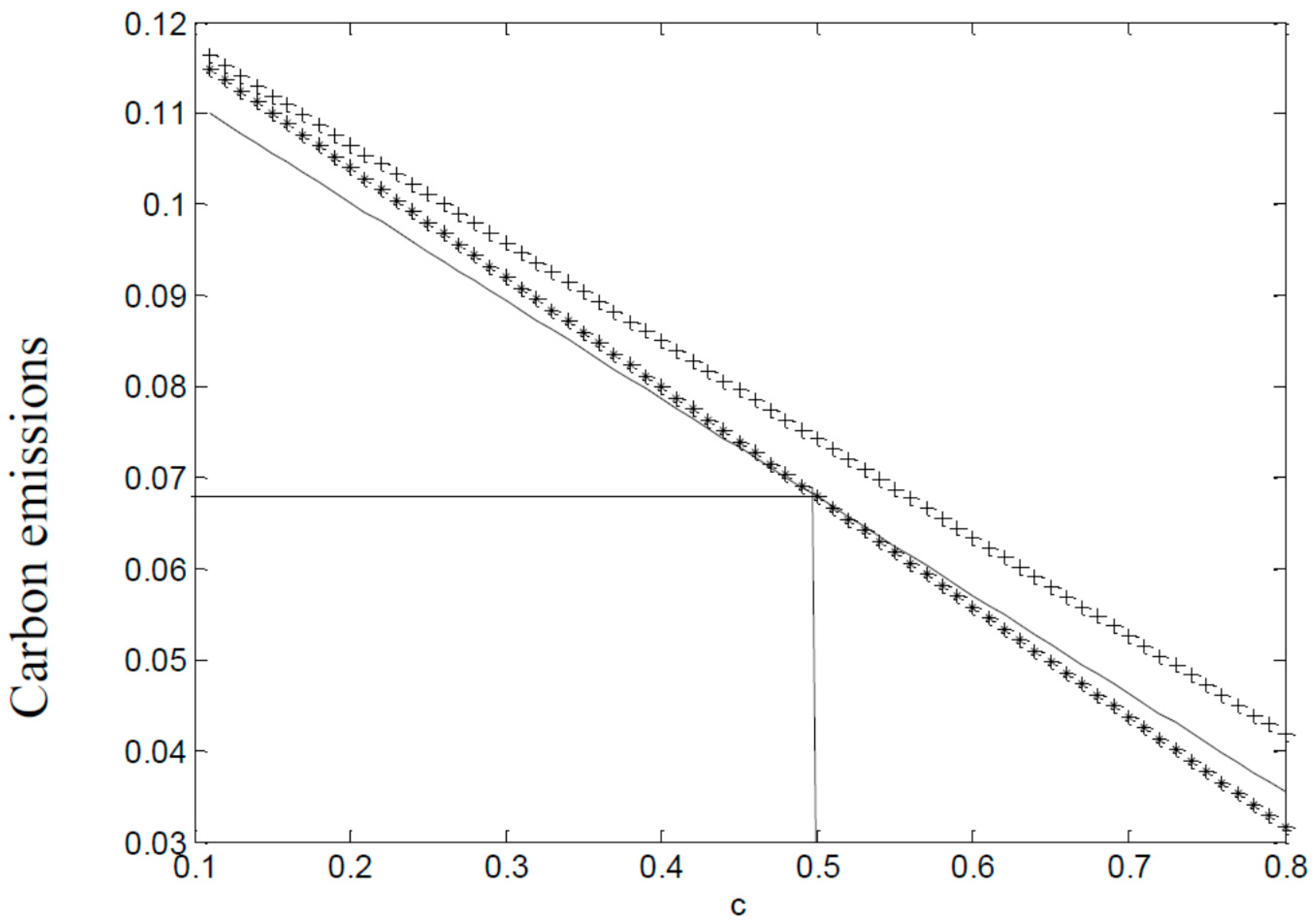
5.2. Comparison of Environmental Impact

The carbon emission of making unit new product is $e_n$, and the carbon emission of making unit remanufactured product is $e_r$, and thus

• In Model N, the total carbon emission is: ${{\rm E}}_N=e_n(q_n^{\alpha N*}+q_n^{(1-\alpha )N*})+e_r(q_r^{\alpha N*}+q_r^{(1-\alpha )N*})$.
• In Model C, the total carbon emission is: ${{\rm E}}_C=e_n(q_n^{\alpha C*}+q_n^{(1-\alpha )C*})+e_r(q_r^{\alpha C*}+q_r^{(1-\alpha )C*})$.
• In Model S, the total carbon emission is: ${{\rm E}}_S=e_n(q_n^{\alpha S*}+q_n^{(1-\alpha )S*})+e_r(q_r^{\alpha S*}+q_r^{(1-\alpha )S*})$.

Observation 6.

When $(1-\rho )c{e}_r\ge s_r$, ${{\rm E}}_N>{{\rm E}}_C>{{\rm E}}_S$; conversely, when $(1-\rho )c{e}_r<s_r$, ${{\rm E}}_N>{{\rm E}}_S>{{\rm E}}_C$. The carbon emission from enterprises is maximal without government subsidy or tax rebate. As a result, the government provides remanufacture subsidy and tax rebate for enterprises to boost remanufacturing development and reduce carbon emissions. Conversely, with the rising government subsidy, enterprises tend to make more products for greater profits. With the rising carbon emission, the government has to set a sensible subsidy to strike a balance between the profit of enterprises and carbon emission.

The proof can be seen in the Appendix A.

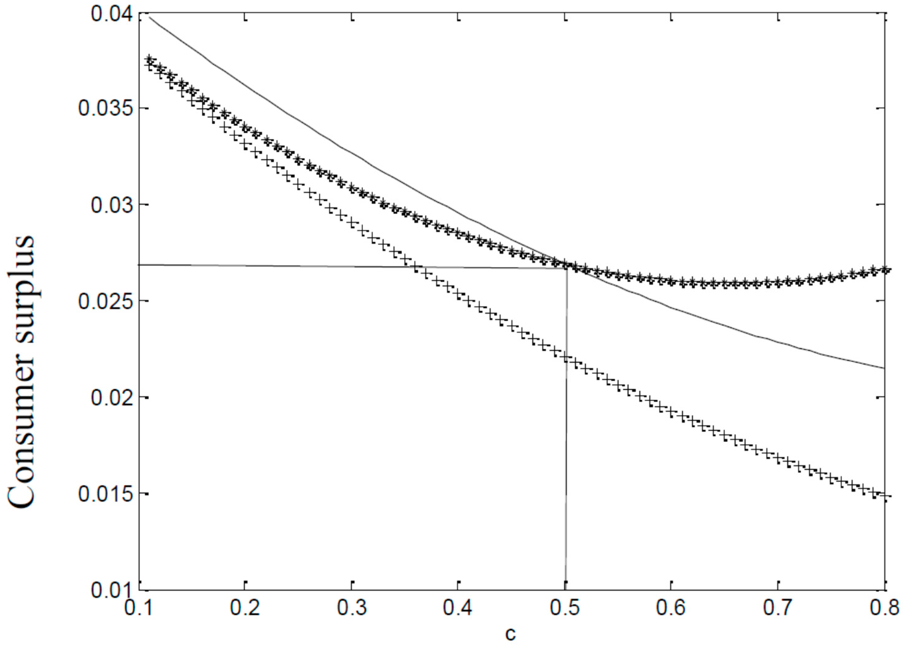
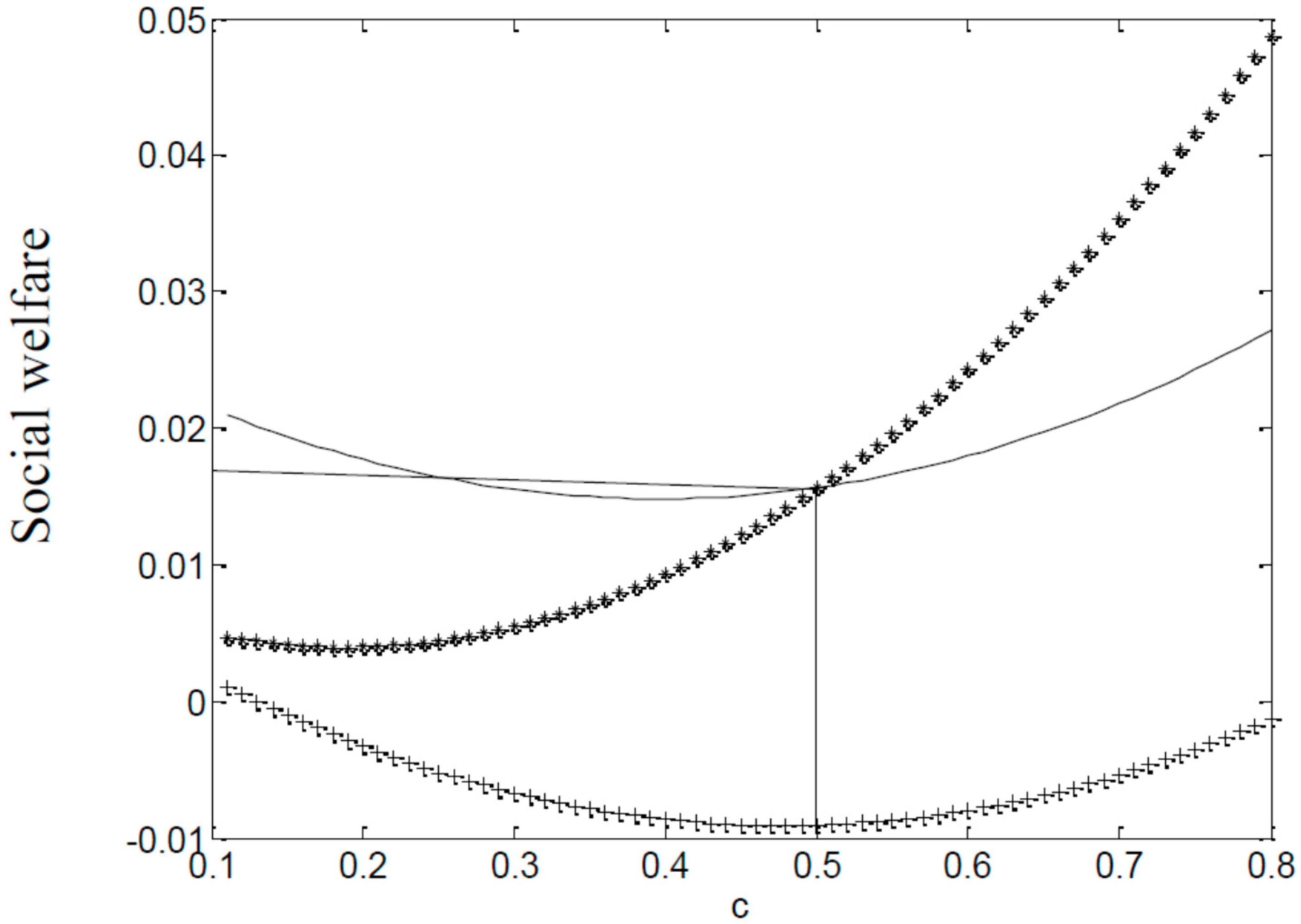
5.3. Comparison of Consumer Surplus and Social Welfare

(1) Consumer surplus $CS={\int }_0^Q\theta d\theta -PQ$. Substituting the optimal value into the equation in each model, in Model N, consumer surplus is $C{S}_N=$($\frac{1+(p_n^{N*}-p_r^{N*})/(1-t)}{2}-p_n^{N*}$)$q_n^{\alpha N*}+$($\frac{p_r^{N*}+t(p_n^{N*}-p_r^{N*})/(1-t)}{2}-p_r^{N*}$)$q_r^{\alpha N*}+$($\frac{1+(p_n^{N*}-p_r^{N*})/(1-t)}{2}-p_n^{N*}$)$q_n^{(1-\alpha )N*}+(\frac{\frac{t(p_r^{N*}-v-s_t)}{t-\delta }+t\frac{p_n^{N*}-p_r^{N*}}{1-t}}{2}-p_n^{N*})q_r^{(1-\alpha )N*}$; in Model C, consumer surplus $C{S}_C=$($\frac{1+(p_n^{C*}-p_r^{C*})/(1-t)}{2}-p_n^{C*}$)$q_n^{\alpha C*}+$($\frac{p_r^{C*}+t(p_n^{C*}-p_r^{C*})/(1-t)}{2}-p_r^{C*}$)$q_r^{\alpha C*}+$($\frac{1+(p_n^{C*}-p_r^{C*})/(1-t)}{2}-p_n^{C*}$)$q_n^{(1-\alpha )C*}+(\frac{\frac{t(p_r^{C*}-v-s_t)}{t-\delta }+t\frac{p_n^{C*}-p_r^{C*}}{1-t}}{2}-p_r^{C*})q_r^{(1-\alpha )C*}$; in Model S, consumer surplus $C{S}_S=$($\frac{1+(p_n^{S*}-p_r^{S*})/(1-t)}{2}-p_n^{S*}$)$q_n^{\alpha S*}+$($\frac{p_r^{S*}+t(p_n^{S*}-p_r^{S*})/(1-t)}{2}-p_r^{S*}$)$q_r^{\alpha C*}+$($\frac{1+(p_n^{S*}-p_r^{S*})/(1-t)}{2}-p_n^{S*}$)$q_n^{(1-\alpha )S*}+(\frac{\frac{t(p_r^{S*}-v-s_t)}{t-\delta }+t\frac{p_n^{S*}-p_r^{S*}}{1-t}}{2}-p_r^{S*})q_r^{(1-\alpha )S*}$

Observation 7.

When $(1-\rho )c{e}_r\ge s_r$, $C{S}_C>C{S}_S>C{S}_N$; conversely, when $(1-\rho )c{e}_r<s_r$, $C{S}_S>C{S}_C>C{S}_N$. The greater the subsidy in the mode means the more consumer surplus.

(2) Social welfare SW = ${\mathrm{\Pi }}_M+CS-{\rm E}$ [15]. Substituting the optimal value into the equation, the social welfare is derived in each model.

Observation 8.

When $(1-\rho )c{e}_r\ge s_r$, $S{W}_C>S{W}_S>S{W}_N$; conversely, when $(1-\rho )c{e}_r<s_r$, $S{W}_S>S{W}_C>S{W}_N$. The greater the subsidy in the mode means the more consumer surplus. Due to the complexity of the equation, the detail is not presented here. In the next section, numerical examples are provided.

The proof can be seen in the Appendix A.

6. Numerical Study

In this section, some numerical examples are used to examine the impact of varying government policies on the profit and carbon emission of enterprises, and thus the analysis of which mode can reduce carbon emission without undermining the profit of enterprises is presented. Based on the previous analysis, we can compare the profit and carbon emission.

6.1. Parameter Design

Following the assumptions in other studies in the literature, the values of parameters in each model are as follows: $c_n=0.4$, $c_r=0.25$, $t=0.7$ (when the manufacturer adopts the strategy of low prices, $p_r<t{p}_n$ is required and the solutions shows that when $c_r<t{c}_n$, it can ensure that there is demand for remanufacturing), $\alpha =0.4$ (when it is assumed that the proportion of replacement customers is greater than that of new consumers, the government provides the subsidy for consumers in the trade-in program to deal with disposal of electronics and other hazardous waste) $s_t=0.2$, $e_n=0.4$, $e_r=0.2$ (remanufacturing is advantages in either cost or carbon emission; since remanufacturing has the advantage in carbon emission, the government provides remanufacture subsidy to boost remanufacturirng development), $\rho =0.5$ (it is assumed that the carbon emission from remanufacturing is half of that from making new products, and thus carbon tax of remanufacturing enjoys 50% of tax rebate), $b=0.1$, $\delta =0.3$, and $s_r=0.05$ (the government subsidizes remanufacturers at 20% of the production cost).

6.2. Result Analysis

It can be seen from Figure 2 that with rising tax rate $c$, the profit of enerprises, with or without subsidy, declines gradually, The carbon tax internalizes the exterior of enterprises as their production cost, and therefore the rising cost means the falling profit. In the case with carbon tax rebate profits have a gradual growth after falling. It suggests that the measuement of carbon emissions of products, the formualtion of scientific and plausible carbon tax with its function of adjustment, tax deduction and exemption or privilege and the return mechanism can gain support from the manufacturer easily. With rising tax rate $c$, the speed of falling profit in the mode of tax rebate from the government is slower than that in the mdoe of remanufacture subsidy from the government. This suggests that when the government concerns the increase of tax rate, the mode of tax rebate suits enterprises better.

Additionally, the figure also shows the same result discussed above: when $(1-\rho )c{e}_r>s_r$, ${\mathrm{\Pi }}_M^C>{\mathrm{\Pi }}_M^S>{\mathrm{\Pi }}_M^N$. Conversely, ${\mathrm{\Pi }}_M^S>{\mathrm{\Pi }}_M^C>{\mathrm{\Pi }}_M^N$. Here, the parameters are: $\rho =0.5$, $e_r=0.2$, and $s_r=0.05$, and thus it can be seen that when $c$ is equal to 0.5, $(1-0.5)\times 0.5\times 0.2=0.05=s_r=0.05$. The profit of enteprises is the same in these two modes. When $c$ is less than 0.5, the profit in the mode of remanufacture subsidy from the government is greater than that in the mode of tax rebate. When $c$ is greater than 0.5, the profit in the mdoe of tax rebate is more than that in the mode of remanufacture subsidy from the government. Consequently, from the perspective of enterprises, the greater amount of subsidy from the government in the particular mode means more profit in that mode. Conversely, regardless of the mode of subsidy, the profit of enterprises with government subsidy is greater than that without the subsidy.

Figure 3 shows that as tax rate $\mathrm{c}$ rises, carbon emission of enterprises declines gradually. The higher carbon tax and the higher carbon emission cost make the manufacturer consider reducing production or turn to producing more environment-friendly product. With rising carbon tax, the reducing speed of carbon emissions in the mode of tax rebate is faster than in mode of remanufacturing subsidy. Additionally, the figure also proves the analysis in the secions discussed above: When $c$ is greater than 0.5, $(1-\rho )c{e}_r\ge s_r$, ${{\rm E}}_N>{{\rm E}}_C>{\mathsf{{\rm E}}}_S$; conversely, when $(1-\rho )c{e}_r<s_r$, ${{\rm E}}_N>{{\rm E}}_S>{{\rm E}}_C$. Greater subsidy in the mechanism means less carbon emission. Consequently, it is indispensible for the government to set the sensible mechanism of subsidy to strike a balance between the profit of enterprises and carbon emissions.

Figure 4 shows that with rising tax rate c, the consumer surplus declines gradually, with or without remanufacturing subsidy. When the government collects carbon tax from enterprises, they transfer part of carbon tax to consumers through pricing decisions. Hence, consumer surplus diminishes with the rise of carbon tax. When there is carbon tax rebate the consumer surplus grows gradully, after falling. It suggests that it is beneficial for consumers if the government formulates scientific and reasonable carbon tax and tax reduction and exemption, and offers privilege and return mechanism. Consumer surplus with government subsidy or carbon tax rebate is greater than that without government subsidy. When $c$ is greater than 0.5, $(1-\rho )c{e}_r\ge s_r$, ${\mathrm{CS}}_N<{\mathrm{CS}}_S<C{S}_C$; conversely, when $(1-\rho )c{e}_r<s_r$, ${\mathrm{CS}}_N<{\mathrm{CS}}_C<C{S}_N$.

It can be seen from Figure 5 that the social welfare increases with the rising tax rate $c$. With the rising tax rate $c$, the production cost of enterprises steps up; their profits decline; carbon emissions drop; and consumer surplus shrinks. Then, why does social welfare increase? The equation of social welfare is SW = ${\mathrm{\Pi }}_M+CS-{\rm E}$, and the three figures above show that, with the rising $c$, the profit, consumer surplus and carbon emission decrease, while the scale and speed of decreasing carbon emission are greater and faster than dropping profits of enterprises and consumer surplus. Thus, the total social welfare is increasing gradually, and social welfare rises fastest particularly in the mode of tax rebate.

The simulation results show that when the government subsidizes manufacturers with remanufacture subsidy or tax rebate, consumers, manufacturers and even the government benefit substantially. In addition, the rising carbon tax rate can increase the social welfare and reduce carbon emission, whereas it can undermine corporate benefits and consumer surplus. As a result, the reduction of carbon emission by increasing carbon tax rate is not the best choice.

7. Conclusions

This article compares the manufacturer’s decision in the single period of two models: the mechanism of the government’s remanufacturing subsidy and the policy of tax rebate. We analyze the manufacturer’s optimal pricing and production decisions under carbon tax and trade-in program. Through detailed analyses and numeric study, this article investigates the impact of the government policy on the optimal decisions of enterprises, environment, consumer surplus, social utility, and many others. These can shed light on the government’s policies and regulations to boost sustainable development and point the direction for enterprises to respond to the relevant government’s policies.

From a holistic perspective, the government as a policy maker wishing to promote remanufacture and proper disposal of hazardous old products has taken many actions, ranging from carbon regulation such as carbon tax and financial incentives such as trade-in subsidy. However, carbon tax can hurt firm profits to some degree, so government has to give a subsidy to balance the profits and carbon emission. Our results show that carbon tax has a great impact on pricing strategies. Trade-in subsidy can encourage customers to replace their existing products with remanufactured products. Both remanufacture subsidy and tax rebate are beneficial to manufacturer and can further promote the remanufacturing development. It is impossible to directly compare and determine whether the mode of remanufacture or that of tax rebate is better. A higher subsidy is more favorable for consumers and manufacturers. Conversely, if carbon tax is high, then relatively speaking, tax rebate is more effective. When carbon tax is relatively high, with the privilege of carbon tax, the profit of enterprises and consumer surplus will fall first and rise later. Thus, after the formulation of the reasonable carbon tax, the privilege of carbon tax is better than the subsidy of remanufacturing in terms of adjustment and thus gains more support from the manufacturer. Therefore, as a policy maker, the government is supposed to introduce sensible mechanisms to increase the profit of each party. Regardless of which mode of subsidy, enterprises should have advantage in remanufacturing cost or in carbon emissions; otherwise, the government’s incentive for the enterprise is insignificant. Consequently, enterprises have to improve their remanufacturing technology to increase their remanufacturing advantages fundamentally.

There are some limitations of this study, alongside many potential research orientations for future studies. The government subsidy is fixed in this article, whereas future studies can take maximizing social welfare as a target and explore how the government can allocate subsidies to maximize social welfare. This article only takes a single period into account, but it does not consider how the salvage influence remanufacturing in the next period through the trade-in program. Thus, the future research can investigate multiple periods and dynamics. This article is concerned with all the relevant policies such as the trade-in program, carbon regulations, remanufacture subsidy and tax rebate implemented by the government. However, in the current market economy, enterprises are more likely to have their rights to choose and make decisions autonomously. Hence, the future research can involve enterprises which autonomously implement some practices such as the launch of the trade-in program or other effective subsidies.

References

1. Mcconocha, D.M.; Speh, T.W. Remarketing: Commercialization of Remanufacturing Technology. J. Bus. Ind. Mark. 1991, 6, 23–37. [Google Scholar] [CrossRef]
2. Ma, W.M.; Zhao, Z.; Ke, H. Dual-Channel Closed-Loop Supply Chain with Government Consumption-subsidy. Eur. J. Oper. Res. 2013, 226, 221–227. [Google Scholar] [CrossRef]
3. Wang, K.; Zhao, Y.; Cheng, Y.; Choi, T.-M. Cooperation or Competition? Channel Choice for a Remanufacturing Fashion Supply Chain with Government Subsidy. Sustainability 2014, 6, 7292–7310. [Google Scholar] [CrossRef]
4. Ferguson, M.E.; Toktay, L.B. The Effect of Competition on Recovery Strategies. Prod. Oper. Manag. 2006, 15, 351–368. [Google Scholar] [CrossRef]
5. Ferrer, G.; Swaminathan, J.M. Managing New and Remanufactured Products. Manag. Sci. 2006, 52, 15–26. [Google Scholar] [CrossRef] [Green Version]
6. Heese, H.S.; Cattani, K.; Ferrer, G.; Gilland, W.; Roth, A.V. Competitive Advantage through Take-Back of Used Products. Eur. J. Oper. Res. 2005, 164, 143–157. [Google Scholar] [CrossRef]
7. Bhattacharya, S.; Savaskan, R.C.; Wassenhove, L.N.V. Closed-Loop Supply Chain Models with Product Remanufacturing. Manag. Sci. J. Inst. Oper. Res. Manag. Sci. 2004, 50, 239–252. [Google Scholar]
8. Gu, Q.L.; Ji, J.H.; Gao, T.G. Pricing Management for a Closed-Loop Supply Chain. J. Revenue Pricing Manag. 2008, 7, 45–60. [Google Scholar]
9. Huang, M.; Song, M.; Lee, L.H.; Ching, W.K. Analysis for Strategy of Closed-Loop Supply Chain with Dual Recycling Channel. Int. J. Prod. Econ. 2013, 144, 510–520. [Google Scholar] [CrossRef]
10. Liu, H.H.; Lei, M.; Deng, H.H.; Leong, G.K.; Huang, T. Quality-Based Price Competition Model for the WEEE Recycling Market with Government Subsidy. Omega 2015, 59, 290–302. [Google Scholar] [CrossRef]
11. Zhu, X.; Wang, M.; Chen, G.; Chen, X. The effect of implementing trade-in strategy on duopoly competition. Eur. J. Oper. Res. 2016, 248, 856–868. [Google Scholar] [CrossRef]
12. Li, K.J.; Xu, S.H. The comparison between trade-in and leasing of a product with technology innovations. Omega 2015, 54, 134–146. [Google Scholar] [CrossRef]
13. Erica, M.O. Trade-Ins, Mental Accounting, and Product Replacement Decisions. J. Consum. Res. 2001, 27, 433–446. [Google Scholar]
14. Zhang, F.; Zhang, P. Trade-In Remanufacturing, Strategic Customer Behavior, and Government Subsidies; Social Science Electronic Publishing: Rochester, NY, USA, 2015. [Google Scholar]
15. Miao, Z.; Fu, K.; Xia, Z.; Wang, Y. Models for closed-loop supply chain with trade-ins. Omega 2015, 66, 308–326. [Google Scholar] [CrossRef]
16. Ray, S.; Boyaci, T.; Aras, N. Optimal Prices and Trade-In Rebates for Durable, Remanufacturable Products. Manuf. Serv. Oper. Manag. 2005, 7, 208–228. [Google Scholar] [CrossRef]
17. Montgomery, W.D. Markets in licenses and efficient pollution control programs. J. Econ. Theory 1972, 5, 395–418. [Google Scholar] [CrossRef]
18. Laffont, J.; Tirole, J. Pollution permits and compliance strategies. J. Public Econ. 1996, 62, 127–140. [Google Scholar] [CrossRef]
19. Benjaafar, S.; Li, Y.; Daskin, M. Carbon footprint and the management of supply chains: Insights from simple models. IEEE Trans. Autom. Sci. Eng. 2013, 10, 99–116. [Google Scholar] [CrossRef]
20. Chen, X.; Benjaafar, S.; Elomri, A. The carbon-constrained EOQ. Oper. Res. Lett. 2013, 41, 172–179. [Google Scholar] [CrossRef]
21. Hua, G.; Cheng, T.C.E.; Wang, S.Y. Managing carbon footprints ininventory management. Int. J. Prod. Econ. 2011, 132, 178–185. [Google Scholar] [CrossRef]
22. Wang, L.; Chen, M. Policies and Perspective on End-of-Life Vehicles in China. J. Clean. Prod. 2013, 44, 168–176. [Google Scholar] [CrossRef]
23. Wang, Y.X.; Chang, X.Y.; Chen, Z.G.; Zhong, Y.G.; Fan, T.J. Impact of Subsidy Policies on Recycling and Remanufacturing Using System Dynamics Methodology: A Case of Auto Parts in China. J. Clean. Prod. 2014, 74, 161–171. [Google Scholar] [CrossRef]
24. Mitra, S.; Webster, S. Competition in Remanufacturing and the Effects of Government Subsidies. Int. J. Prod. Econ. 2008, 111, 287–298. [Google Scholar] [CrossRef]
25. Miao, Z.; Mao, H.; Fu, K.; Wang, Y. Remanufacturing with trade-ins under carbon regulations. Comput. Oper. Res. 2017, in press. [Google Scholar] [CrossRef]
26. Shi, W.; Min, K.J. Remanufacturing decisions and implications under material cost uncertainty. Int. J. Prod. Res. 2014, 53, 6421–6435. [Google Scholar] [CrossRef]
Figure 1. Closed-loop supply chain models.
Sustainability 09 00156 g001
Figure 2. Manufacturers’ profits with respect to tax rate c . — manufacturers’ profits with remanufactured subsidy; *** manufacturers’ profits with tax rebate; +++ manufacturers’ profits without government subsidy.
Sustainability 09 00156 g002
Figure 3. Carbon emission of manufacturer with respect to tax rate c . — carbon emissions with remanufactured subsidy; *** carbon emissions with tax rebate; +++ carbon emissions without government subsidy.
Sustainability 09 00156 g003
Figure 4. Consumer surplus of manufacturers with respect to tax rate c . — consumer surplus with remanufactured subsidy; *** consumer surplus with tax rebate; +++ consumer surplus without government subsidy.
Sustainability 09 00156 g004
Figure 5. Social welfare of manufacturer with respect to tax rate c . — social welfare with remanufactured subsidy; *** social welfare with tax rebate; +++ social welfare without government subsidy.
Sustainability 09 00156 g005