A Quantitative Groundwater Resource Management under Uncertainty Using a Retrospective Optimization Framework

Abstract

Water resources are a major concern for any socio-economic development. As the quality of many surface fresh water sources increasingly deteriorate, more pressure is being imparted into groundwater aquifers. Since groundwater and the aquifers that host it are inherently vulnerable to anthropogenic impacts, there is a need for sustainable pumping strategies. However, groundwater resource management is challenging due to the heterogeneous nature of aquifer systems. Aquifer hydrogeology is highly uncertain, and thus it is imperative that this uncertainty is accounted for when managing groundwater resource pumping. This, therefore, underscores the need for an efficient optimization tool which can sustainably manage the resource under uncertainty conditions. In this paper, we apply a procedure which is new within the context of groundwater resource management—the Retrospective Optimization Approximation (ROA) method. This method is capable of designing sustainable groundwater pumping strategies for aquifers which are characterized by uncertainty arising due to scarcity of input data. ROA framework solves and evaluates a sequence of optimization sub-problems in an increasing number of realizations. We used k-means clustering sampling technique for the realizations selection. The methodology is demonstrated through application to an hypothetical example. The optimization problem was solved and analyzed using “Active Set” algorithm implemented under MATLAB environment. The results indicate that the ROA sampling based method is a promising approach for optimizing groundwater pumping rates under conditions of hydrogeological uncertainty.

1. Introduction

Many parts of the world are experiencing acute freshwater shortages in terms of both quality and quantity due to various factors such as variability of the hydrological cycle and the climate, and ever increasing population and anthropogenic influences. An increase in water demand for irrigation, domestic, and industrial use, as well as the conflicting demands for sustainability of the ecosystem, has posed great pressure on water natural storage systems. An increase in water demands due to ever increasing population and environmental degradation coupled with variability of the hydrological cycle and the climate has resulted in over extraction of the limited water resources in many parts of the world. As surface water quality increasingly deteriorates, more pressure is turned to groundwater aquifers to sustain the ever increasing water demands. In the arid and semi-arid regions groundwater represents a vital resource which most people rely on, which can cover the shortage of water caused by uneven distribution of the surface water in time and space [1]. Moreover, in the agricultural sector the over-pumping of groundwater resources for sustaining crops and livestock is inevitable [2]. However, overexploitation of these natural water reservoirs has many adverse impacts, such as ground surface subsidence and fresh sea water intrusion into coastal aquifers.

To circumvent these undesirable effects, it is important to understand the behavior of the groundwater aquifer system when subjected to external excitations (such as pumping). This coupled with a sustainable groundwater pumping (i.e., optimal pumping rates) strategy will ensure efficient exploitation of groundwater resources. It should be realized that optimal pumping of a groundwater resource requires that the groundwater (aquifer) reservoir must be fully characterized if deterministic approaches are to give reliable results. Moreover, detailed hydrogeological data in space and time, which are usually obtained by a large number of field experiments, are typically required to construct physical models in practical application [1]. However, in reality, full characterization of aquifers (groundwater) is neither practically possible nor economically feasible [3], hence alternative approaches are required which are capable of utilizing the available scanty data so as to design pumping strategies which recognize the uncertainty due to inadequacy of data.

Our main contribution in this paper is to present a combined simulation optimization methodology (stochastic optimization approximation sampling based methods—Retrospective Optimization Approximation (ROA) framework) which considers the geological uncertainty brought about by lack of adequate data to fully characterize the groundwater aquifer system. Since groundwater resource management is generally carried out in an environment of uncertainties, it is imperative that uncertainty is addressed for reliable groundwater management planning and decision making. Heterogeneity in natural aquifer formations is widely recognized as one of the major factors contributing to uncertainty in predicting groundwater flow behavior [4], and management strategies [3]. However, it should be noted that the incorporation of a simulation model within an optimization-based management model is complex and difficult, and takes considerably large computational time to achieve any optimal solution [5]. An embedding technique or response matrix approach is usually used to incorporate a simulation model within management optimization models [6].

The embedding technique for solving groundwater management problems was first invented by Aguado and Remson [7]. In this approach, numerical approximations of the flow equations are included directly as constraints in the optimization model [3,7]. Thus, each element within the modeled domain is represented by an equation in the optimization problem, and consequently leads to a huge optimization problem, which is the main disadvantage to its application [3]. The response matrix approach uses superposition and linear systems theory to simulate groundwater flow [8]. In the response matrix approach, also known as technological matrix approach, the influence of a unit change in an independent decision variable, such as pumping at a pre-selected well location, upon a variety of dependent variables, like drawdown at specified potential control observation points, is determined. Then, the superposition process is performed to calculate their total response at specified potential control points resulting from all decision variables [3].

In other words, a response matrix consists of linear influence coefficients that describe the response of the potentiometric surface to a unit volume of extraction or injection of groundwater [8]. The main shortcoming of this approach is in regards to the number of simulations needed to be performed to generate the response (the size of the response matrix is a function of stress locations and observation points considered). However, the final optimization problem to be solved is smaller than that which can be obtained from the embedding method [3]. In this work, we adopted a response technique for combining a simulation model with an optimization model (procedure).

It should be realized that traditionally solving simulation optimization problems under uncertainty is computationally expensive, because many flow simulations are required to provide reliable results. Wang et al. [9] asserted that efficient treatment of uncertainty, particularly geological uncertainty, presents a key challenge in the application of optimization procedures, and further emphasized that the reason behind this is that in order to present the high degree of uncertainty in the reservoir geology many geological realizations must be considered. In groundwater management, a number of methodologies have been developed and published in the literature to address uncertainty, these include post optimality analysis (e.g., [10,11,12]), and stochastic optimization with recourse method as presented by [3,13,14]. However, it should be noted that direct application of such an approach in which all realizations are considered at each iteration of the optimization leads to very costly optimizations, particularly when the number of realizations is large [9]. The aim of this paper is to introduce and apply an efficient method—the ROA framework for optimizing groundwater pumping rates over multiple hydrogeological model realizations. Our work is based on stochastic optimization using a recent refinement of sample average approximation (SAA) sampling based methods—the ROA method (where optimization sub-problems are designed through expected functions and evaluated in a sequence of increasing numbers of realizations).

In general, the basic idea of ROA is that it does not consider all realizations at all iterations of the optimization solver. Instead, the ROA framework defines a sequence of approximate sample path optimization sub-problems, which sequentially account for increasing numbers of hydrogeological realizations. The ROA procedure takes the advantage of the “warm start” technique whereby an initial solution (guess) is updated by considering that the initial solution for the current sub-problem is simply the return solution from the previous sub-problem solved. This technique is new in areas of groundwater resource management, however, in recent years the method has predominantly been used in other fields of studies such as petroleum engineering (for example, for considering well placement optimization problem [9,15,16,17,18], well control problem [19,20]), and in areas of operation research [21,22].

However, their applications were based upon fixed and relatively few decision variables and numbers of realizations. The ROA technique applied here differs from the previous approaches in the sense that it is applied to solve a sequence of optimization sub-problems (particularly designed for consideration of the groundwater resource management problem under geological uncertainty) in an increasing number of realizations of hydrogeological model realizations (i.e., through the response matrix simulation optimization technique).

This paper is generally organized as follows: Firstly, we present the problem of groundwater resource management under uncertainty. Then, a description of the ROA framework is discussed. After that, the hypothetical aquifer system and the application result that demonstrate the effectiveness of the ROA framework are discussed and graphically presented. The application results show the promising computational advantage of the ROA procedure.

2. Materials and Methods

2.1. ROA for Groundwater Resource Management

2.1.1. Optimization Problem

We seek to optimize the groundwater quantity pumping rates of a number of spatially distributed pumping wells under hydrogeological uncertainty conditions, particularly uncertainty due to aquifer hydraulic conductivity field. In this case, uncertainty is expressed in terms of the assemblage of aquifer system responses (drawdowns, which are determined under hydraulic conductivity field uncertainty conditions) due to unit groundwater pumping stress at every potential candidate pumping well location in the model domain. This assemblage set of response values (also known as response matrix coefficients) are normally developed in view to represent a simulation model in a simulation optimization framework.

Now, let hydraulic conductivity field uncertainty realization be denoted by $\varpi$, such that $\varpi \in \mathsf{\Omega }$, where $\mathsf{\Omega }$ is the total possible number of realizations, thus each realization $\varpi$ will have a different random response matrix denoted by $A_{\varpi }$ with associated random response matrix components denoted by $a_{i,j,\varpi }$. Hence, the random response matrices generated may result in different optimal solutions and, therefore, different optimal values of the optimization problem. In general, the optimization problem under uncertainty can be formulated as follows. For a given solution set $X,$such that$X^{*}\in X$, $\mathit{x}\in X,$find a solution $X^{*}$ that

$$Maximize \left[f\left(\mathit{x}\right)= {{\displaystyle \sum }}_{j=1}^{N_{pw}}{x}_j\right], j= 1,2, \dots , N_{pw}$$

(1)

Subject to:

$${\mathbb{E}}_{\mathsf{\Omega }}\left[G\left(x_j,A_{\varpi }\right)\right]\le b_i, i=1,2, \dots , N_c; \forall \varpi \in \mathsf{\Omega }$$

(2)

where ${\mathbb{E}}_{\mathsf{\Omega }}$ represents the expectation function over the set of all realizations $\mathsf{\Omega }$, and $G$ is a numerical stochastic process that computes the sample observation of constraint function $G\left(x_j,A_{\varpi }\right)$ for a given $\mathit{x}$ and the realization $\varpi$.

In this case, $\mathit{x}$ is the vector defining the groundwater pumping rates spatially distributed over the model domain; $f\left(\mathit{x}\right)$ is objective function evaluated through estimates of $G\left(x_j,A_{\varpi }\right)$ function by performing a numerical flow simulation with the hydrogeological model defined by realization $\varpi$; $x_j$ is the groundwater pumping rate (decision variable) of a pumping well located at $j$; $b_i$ is a constraining value at control point $i$; $N_{pw}$ and $N_c$ are the number of pumping wells and control points, respectively. It should be noted that the pumping well locations which were considered for developing response matrices are the same in all realizations.

Consider a random response matrix defined by $A_{\varpi }$ with random response matrix components denoted by $a_{i,j,\varpi }$ (simply denoted by $\overline{\varpi }$), which is the random hydraulic heads/water table level drawdowns. We assume that randomness in hydraulic heads/water table level drawdowns is only due to uncertainty arising in hydraulic conductivity of the aquifer system and that $a_{ij,\varpi }\in A_{\varpi }$ such that $A_{\varpi }\in \overline{\mathsf{\Omega }}$. Moreover, we assume that $\mathrm{P}$ is well defined and a known distribution, but expected mean values and/or covariance of the random responses $\overline{\varpi }$ are known. We consider a stochastic constraint function process as $\mathrm{G}\left(x_j, \overline{\varpi } \right)\in \overline{\mathsf{\Omega }}$ to be defined as $\mathrm{G}\left(x_j, {\overline{\varpi }}_i \right)= A_{{\varpi }_i} x_j$. Thus, the expected value of the function $\mathrm{G}\left(x_j, \overline{\varpi } \right)$is defined as:

$$\mathbb{E}\left[\mathrm{G}\left(x_j, \overline{\varpi }\right)\left]= \mathbb{E}\right[A_{\varpi } x_j\right]$$

(3)

Hence, the constraint inequality (2) can be written as $\mathbb{E}\left[\mathrm{G}\left(x_j, \overline{\varpi }\right)\right]\le { \mathrm{b}}_i$ such that the expectation $\left[\mathrm{G}\left(x_j,\overline{\varpi }\right)\right]= {{\displaystyle \int }}_{\overline{\mathsf{\Omega }}} \mathrm{G}\left(x_j, \overline{\varpi }\right)\mathrm{dP}\left(\overline{\varpi }\right)$ is the corresponding expected value function. Therefore, inequality (2) can be estimated by using Monte Carlo sampling based approximation methods (in this case the ROA method) by considering a sequence of a finite set of generated independent and identically distributed ($i.i.d.$) samples of random response matrices of $N$ realizations of $\overline{\varpi }=\left\{A_{{\overline{\varpi }}_{N_1}}, \dots , A_{{\overline{\varpi }}_{N_k}}\right\}.$ We estimated the expected constraint function $\mathbb{E}\left[\mathrm{G}\left(x_j, {\overline{\varpi }}_{i_k}\right)\right]$as

$$g_{N_k}\left(\mathit{x}\right)=\mathbb{E}\left[\mathrm{G}\left(x_j, {\overline{\varpi }}_{i_k}\right)\right]=[\frac{1}{N_k}{{\displaystyle \sum }}_i^{N_k}\mathrm{G}(x_j,{\overline{\varpi }}_{i_k})]$$

(4)

then progressively evaluated resulting sample path optimization sub-problems using the ROA method framework for $k = 1, 2, \dots ,N_{SP}$; where $N_{SP}$ is the number of sample path optimization sub-problems generated. Hence, the Estimates Retrospective Groundwater Sample path Optimization Problem (ERGSOP) can be formulated as

$$Maximize \left[f_{N_k}\left(\mathit{x}\right)= {{\displaystyle \sum }}_{j=1}^{N_{pw}}{x}_j\right], j= 1,2, \dots , N_{pw}$$

(5)

Subject to:

$$[\frac{1}{N_k}{{\displaystyle \sum }}_{\mathrm{i}}^{N_k}\mathrm{G}(x_j,{\overline{\varpi }}_{i_k})] \le b_{i }$$

(6)

The estimates inequality function (6) is deterministic and hence the optimization sub-problems developed becomes deterministic which can be solved by any appropriate core deterministic search optimizer algorithm. This is one of the main advantages of the ROA approach. It should be noted that the ROA procedure can be used in deterministic and stochastic search algorithms [8]. The optimization problems formulations (1) through (2) and problem formulation (5) through (6) are herein referred to as the true optimization problem and estimates optimization problem, respectively.

In inequality (6), the term $\frac{1}{N_k}$ defines the weight factor or probability associated with realizations ${\overline{\varpi }}_{i_k}$. In this work, different sample sizes $N_k$ (number of realizations) were considered for each sample path optimization sub-problem generated. The performance objective function considered is the expected total optimal groundwater pumping rate. Decision variables considered are groundwater pumping rates (i.e., positive real values $X$, such that $X\in {\mathsf{ℝ}}^{Npw}$) which are spatially distributed within the model domain. In this case, we assume that the solution set $X$ is closed and bounded, and hence the problem has a finite number of feasible solutions.

2.1.2. ROA Framework

The basic feature of the ROA framework is that the sample sizes (i.e., the number of realizations) are increased from sample path optimization sub-problem to sub-problem, and that the initial guess solution for the current sample path optimization sub-problem is simply the returned solution from the previous sample path optimization sub-problem solved. This guarantees that in early iterations, the ROA procedure does not require excessive computational effort because the number of realizations (sample sizes) is small. Similarly, in the later iterations it is computationally inexpensive because the initial solutions are closer to the optimum solution of the true optimization problem. Hence, the overall iterations required by the core optimizer are relatively fewer, and therefore, computational savings can be achieved compared to a direct optimization which considers all realizations at each iteration.

In order to solve the stochastic optimization problem using the Retrospective Optimization Approximation (ROA) approach, the following elucidated steps are followed:

(1)

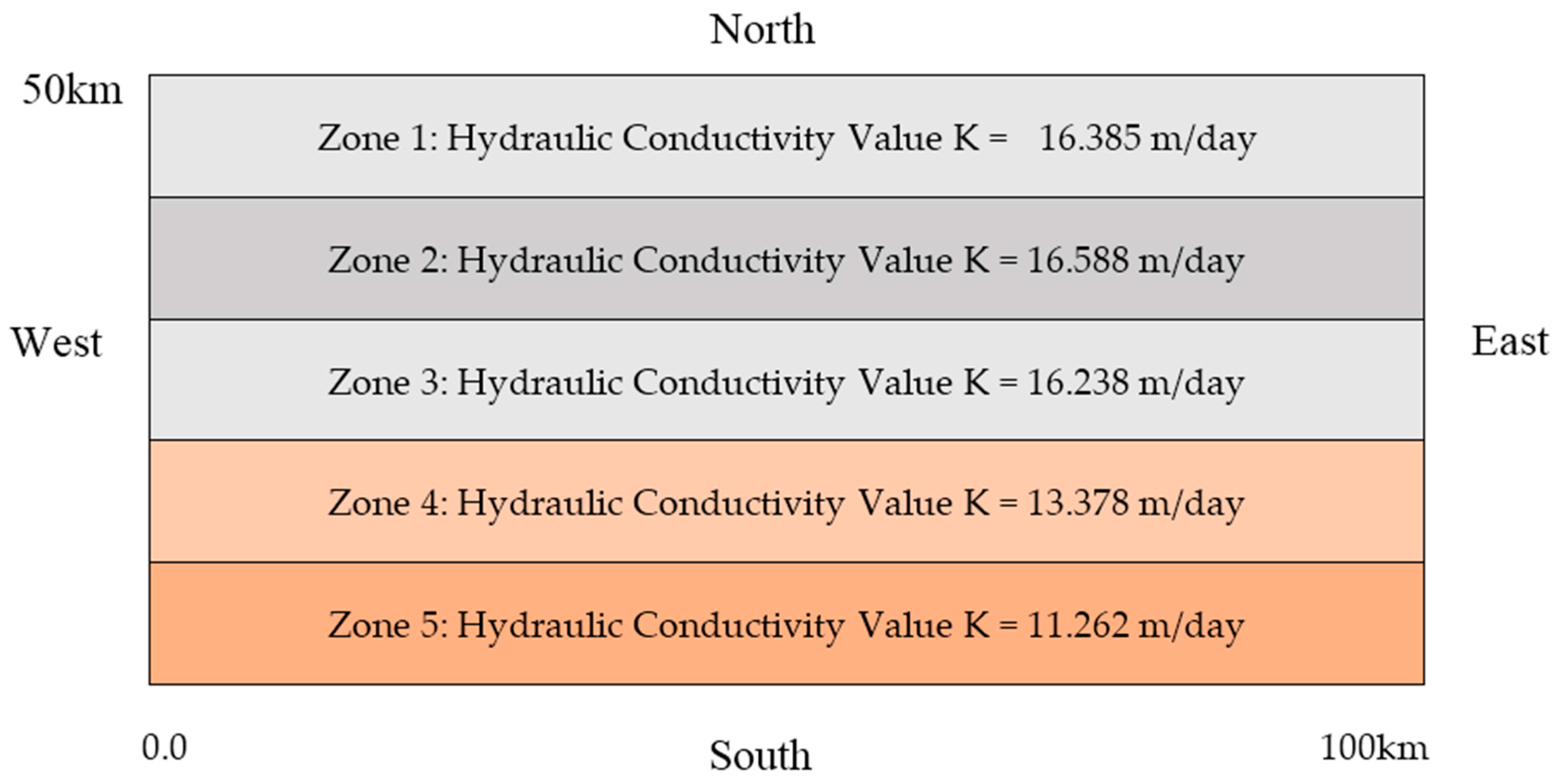
For a given available data (in this case hydraulic conductivity field mean, standard deviation) generate set of realizations of aquifer hydraulic conductivity fields $\varpi$.

(2)

For each given realization $\varpi ,$ run the MODFLOW simulation model to generate responses$a_{ij,\varpi }$ (i.e., $\overline{\varpi }$ random responses of hydraulic heads/water table level drawdowns) due to a unit groundwater pumping rate (we consider existing maximum groundwater pumping rate to represent a unit pumping rate).

(3)

Generate a sequence of a finite set of independent identically distributed $\left(i.i.d.\right)$ samples of random aquifer response matrices $A_{\varpi }$ of $N$ realizations of $\left\{{\overline{\varpi }}_{N_k}\right\}=\left\{A_{{\overline{\varpi }}_{N_1}}, \dots , A_{{\overline{\varpi }}_{N_k}}\right\}$, for$k = 1, 2, \dots ,N_{SP}$.

(4)

For a given sequence of a finite set of the generated samples of aquifer response matrices realized generate a sequence of retrospective sample path sub-problems $f_{N_k} , for k=1,2,\dots , N_{SP}$.

(5)

For each kth sample path sub-problem apply core optimizer solver to provide an optimal solution (or a nearly closer approximation of optimal solution) $X_k$ of $f_{N_k}$.

Repeat step (5) for $k = 1, 2, \dots , N_{SP}$ until sample path optimization sub-problem optimal solution $X_k^{*}$ converges to true optimization problem optimal solution$X^{*}$. Note that for each sub-problem we consider the distinct probable weight factor of $pr\left({\overline{\varpi }}_{N_k}\right)=\frac{1}{N_k}$, hence as $\mathrm{k}$ increases, the sample path sub-problem $f_{N_k}$ optimal solution $X_k^{*}$ converges to the true optimization problem optimal solution $X^{*}$ of objective function$f$.

2.1.3. Sampling Technique

Various sampling strategies can be applied to the ROA framework depending on the availability of data. In this hypothetical example, we apply a k-means clustering algorithm implemented in MATLAB 2014a environment. In k-means clustering sampling, we established mapping from every realization to a finite number $n$ of attributes. From a groundwater pumping water production perspective, hydraulic conductivity is an attribute that can be useful to measure. Firstly, the quantity is normalized to [0, 1] and then a vector of values is assigned to each realization. Using this process, we were able to identify each realization of hydraulic conductivity field, ${\varpi }_i,$ with a vector of attributes${\rho }_i$,${\rho }_i\in {\mathsf{ℝ}}^n$. The vectors of the attributes are then used in the k-means algorithm. The k-means algorithm provides $k$ vectors in ${\mathsf{ℝ}}^n$ (i.e., cluster centers) that minimize mean (average) distance $d$ for a given $N$ numbers of realizations, and can be defined in the form:

$$d= {{\displaystyle \sum }}_{i=1}^{n}min\Vert {\rho }_i-{\varphi }_j\Vert {}^2, j=1,2, \dots , k$$

(7)

where ${\rho }_i$ denotes a vector of attributes such that ${\rho }_i\in {\mathsf{ℝ}}^n$; and ${\varphi }_j$ denotes the coordinates of the center of cluster $j$. For the k-means approach once the cluster centers are established, a particular realization ${\varpi }_i$ is assigned to one of the centers by simply computing the minimum distance as $ar{g}_{mi{n}_{j=1,2,...,k}}\Vert {\rho }_i-{\varphi }_j\Vert$.

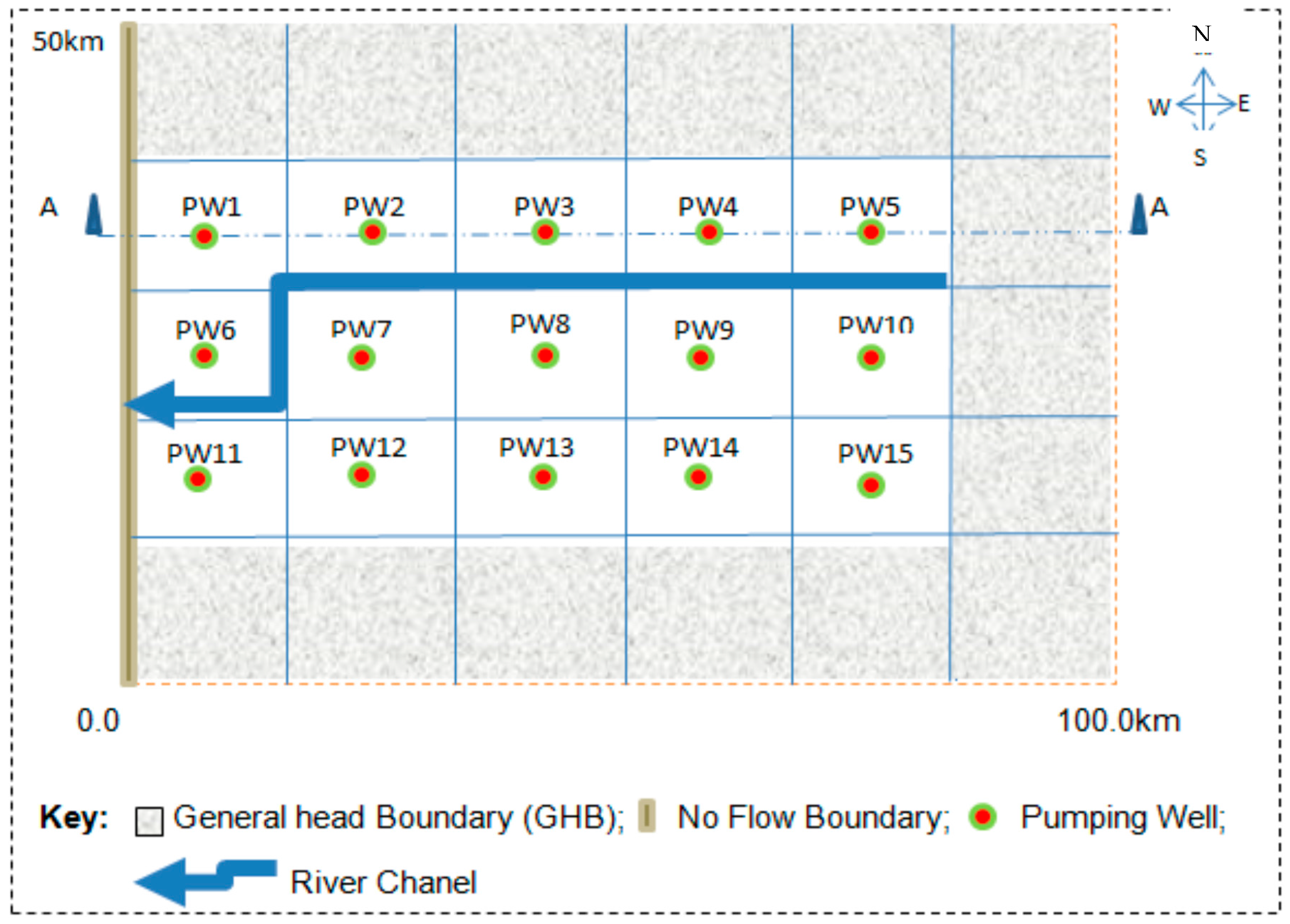
2.2. Application of ROA Framework

The ROA methodology (management tool) developed is general in scope and can be applied to real or hypothetical aquifer systems by considering a sequence of increasing sample sizes of the sample path optimization sub-problems. In this work, the proposed ROA methodology was applied to a modified hypothetical aquifer water system after [23] to comprehensively illustrate a quantitative groundwater resource hydraulic management problem. The hypothetical aquifer water system consisted of a river system, groundwater pumping wells, and agricultural fields. The model was formulated to represent realistic hydrology and hydrogeology of an aquifer water resource system, but does not represent any real basin. Therefore, the physical features modelled are general in nature. The hypothetical aquifer water system has a rectangular areal extent of 100.0 km by 50.0 km which was uniformly discretized into 30 grid cells in 5 rows and 6 columns with an equal grid spacing of 16.67 km in the x-direction and 10.0 km in the y-direction. The finite difference method was used to discretize the area. In general, the size of the model domain area represented by the model can be classified as a relatively small area, which is approximately 5000.00 km². The aquifer system is characterized by relatively low hydraulic conductivity. Figure 1 shows the heterogeneous aquifer hydraulic conductivity values adopted after [23], classified into five (5) zones.

It was assumed that the aquifer has no-flow boundary conditions on the western part. On the east, north, and south parts of the model domain, boundaries provide a controlled general head flow boundary (GHB). The potential groundwater pumping wells are located in 15 internal active model domain grid cells as shown in Figure 2. Aquifer heads at these potential groundwater pumping wells (PWs) were restricted by not allowing them to fall below 50 percent of the specified saturated aquifer thicknesses (i.e., not allowing them to fall below maximum allowable total drawdowns). Figure 2 shows the finite difference groundwater conceptual schematic layout diagram.

The aquifer system has an average saturated thickness ranging from 93.50 m to 135.20 m. Figure 3 shows a groundwater conceptual hydrogeological unit cross-sectional area of the cross section A–A (see Figure 2).

In this example, it was assumed that irrigation is the only water use. The irrigated area receives water mainly from the groundwater pumping wells. Recharge to the groundwater body from the fields was adopted as 7.5 percent of application losses and net recharge was estimated at a rate of 106 mm/year [23].

Table 1. River and Aquifer Properties Model Inputs Parameters.

Item	River/Aquifer System Property	Parameter Value
1	Mean Riverbed Hydraulic Conductivity	0.2 m/day
2	Mean River Width Ranges	80 m–100 m
3	Mean Riverbed Thickness Ranges	2 m–3 m
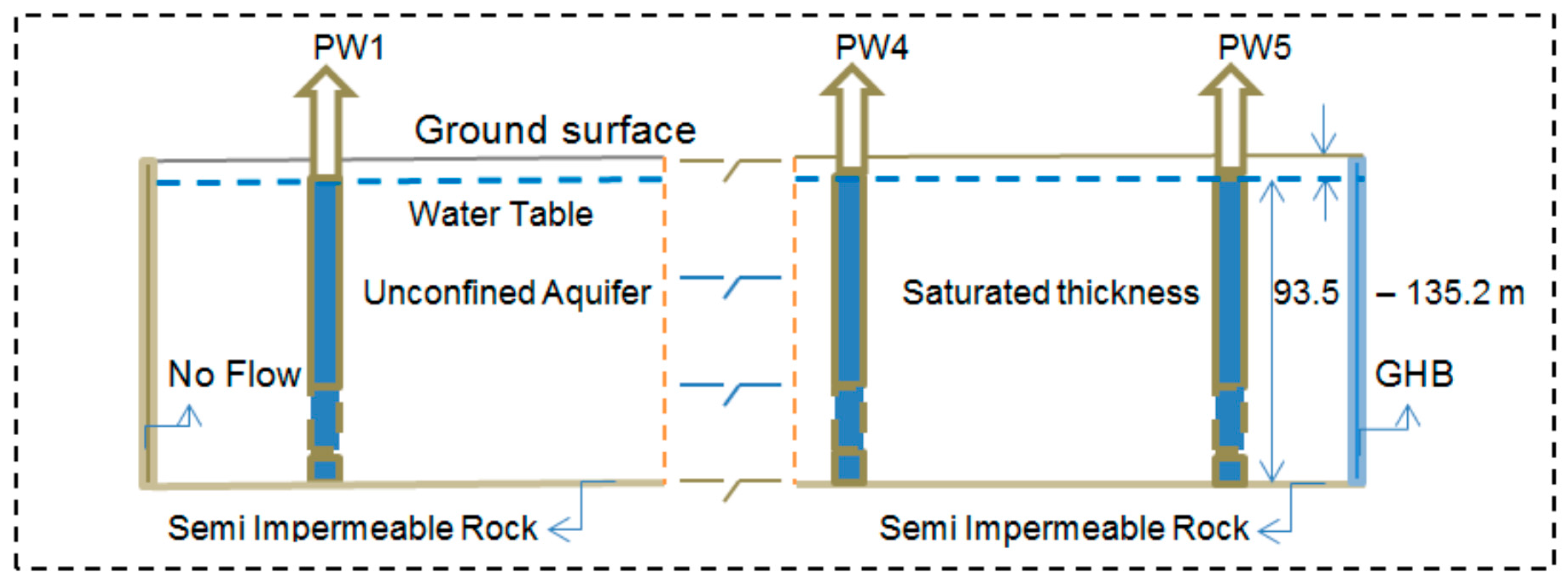
4	Mean Aquifer Saturated Thickness Ranges	93.50 m–135.20 m
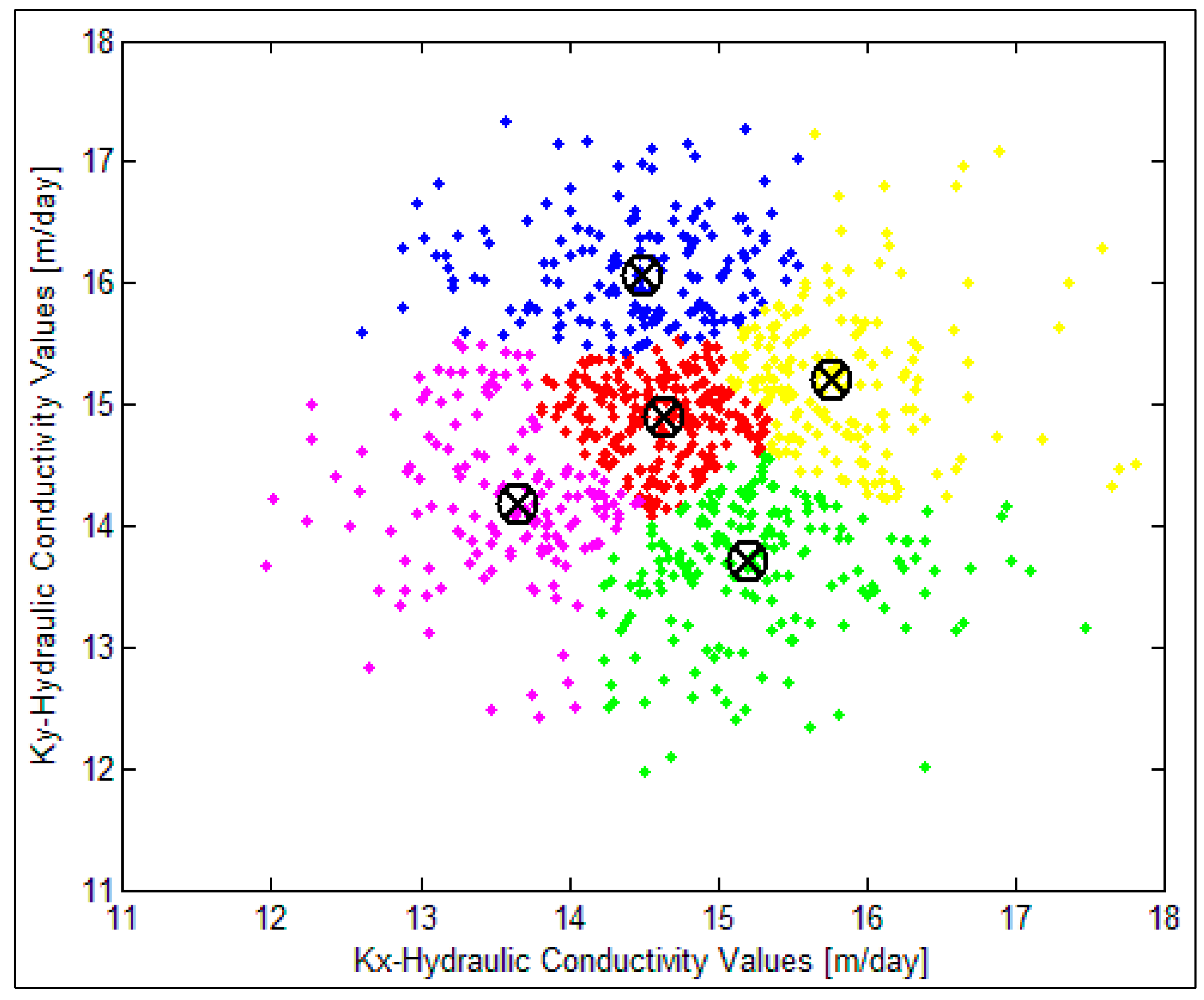
5	Mean Aquifer Hydraulic Conductivity	14.77 m/day
6	Mean Aquifer Specific Yield	0.1
7	Total Annual Aquifer Net Recharge	106 mm/year

summarizes the river and aquifer properties data adopted after [23], which were used for the hypothetical optimization problem.

The overall modelling effort was to manage the water resources, particularly the groundwater resource of the aquifer system in such a manner so as to maximize groundwater pumping production rates without substantially imparting undesirable consequences onto the ecosystem. To achieve this goal, the following objective and constraints were considered:

● Objective

The objective was formulated as follows:

$$Maximise \left[Z= {{\displaystyle \sum }}_{j=1}^{N_{pw}}{x}_j\right], j= 1,2, \dots , N_{pw}$$

(8)

where $Z$ is the objective function value that represents the total groundwater pumping rate; $x_j$ are the spatially distributed pumping rates (decision variables); and $N_{pw}$ is the total number of potential pumping wells.

● Constraints

The objective function was constrained with the following constraints:

Drawdown constraints—Drawdown constraints are usually meant to protect the ecosystem by avoiding excessive drawdowns. In this work, the drawdown constraints were formulated to avoid mining, as follows:

$${{\displaystyle \sum }}_{j=1}^{N_{pw}}{a}_{i,j}{x}_j \le b_i; i=1,2, \dots , N_c$$

(9)

where $a_{i,j}$ is the drawdown at control point $i$ caused by a unit pumping from potential pumping well located at $j$; $b_i$ is the allowable drawdown at control point $i$; and $N_c$ is the total number of control points (control points are location points at which the drawdowns are controlled).

As noted, the aquifer hydraulic conductivity values are considered to be uncertain, hence, the drawdowns $a_{i,j}$ become dependent on the hydraulic conductivity field, $\varpi$, realized. As previously mentioned, the assemblage of the random response coefficients $a_{i,j,\varpi }$ forms a finite set of independent identically distributed $\left(i.i.d.\right)$ samples of random aquifer response matrices $A_{\varpi }$ of $N$ realizations as $\left\{ A_{{\varpi }_{N_k}}\right\}=\left\{A_{{\overline{\varpi }}_{N_1}}, \dots , A_{{\overline{\varpi }}_{N_k}}\right\}$, for $k = 1, 2, \dots ,N_{SP}$. Therefore, inequality (9) changes to the following form:

$$A_{{\varpi }_{N_k}}{x}_j= \le b_i; i=1,2, \dots , N_c; k=1,2, \dots , N_{SP} ; \forall \varpi \in \mathsf{\Omega }$$

(10)

In this case, the stochastic inequality constraint (10) can be estimated as:

$$\frac{1}{N_k}{{\displaystyle \sum }}_{k=1}^{N_k}{A}_{{\overline{\varpi }}_{N_k}} x_j= \le b_i; i=1,2, \dots , N_c$$

(11)

where $A_{{\overline{\varpi }}_{N_k}}$ is the kth sample path optimization sub-problem constraints response matrix, and all other parameters are as previously defined.

Total recharge constraint—The total amount of water extracted from the aquifer was constrained so as not to exceed the total natural recharge entering the aquifer model domain. This constraint was considered to be a hard constraint and was formulated as:

$${{\displaystyle \sum }}_{j=1}^{N_{pw}}{x}_j \le R_T$$

(12)

in which $R_T$ is the total recharge in the well field.

Water demand constraint—In this work, the aquifer was considered as the sole source of water supply. Hence, it means that the designed optimal pumping strategy must satisfy at least the minimum total water demand without impacting negatively on the other water sources. The constraint was formulated as follows:

$${{\displaystyle \sum }}_{j=1}^{N_{pw}}{x}_j \ge W{D}_{T }$$

(13)

where $W{D}_T$ is the total water demand within the model domain.

Pumping constraint—Pumping rates at each potential pumping well were constrained to values between some minimum and maximum rates. This constraint was formulated as follows:

$$x_j^{min} \le x_j \le x_j^{max} ; j=1,2, \dots , N_{pw}$$

(14)

where $x_j^{min}$ and $x_j^{max}$ are the minimum and maximum allowable pumping rates, respectively.

● Statement of the Management Problem

The stochastic optimization problem solved, therefore, was as follows:

$$Maximize \left[Z= {{\displaystyle \sum }}_{j=1}^{N_{pw}}{x}_j\right], j= 1,2, \dots , N_{pw}$$

(15)

Subject to:

$$A_{{\varpi }_{N_k}}{x}_j= \le b_i; i=1,2, \dots , N_c; k=1,2, \dots , N_{SP} ; \forall \varpi \in \mathsf{\Omega }$$

(16)

$${{\displaystyle \sum }}_{j=1}^{N_{pw}}{x}_j \le R_T$$

(17)

$${{\displaystyle \sum }}_{j=1}^{N_{pw}}{x}_j \ge W{D}_T$$

(18)

$$x_j^{min} \le x_j \le x_j^{max} ; j=1,2, \dots , N_{pw}$$

(19)

The optimization problem formulation (15) through (19) is a stochastic optimization problem because it depends on the realization of hydraulic conductivity field$\varpi$. This optimization problem is referred to as the true groundwater optimization problem. The estimates sample path optimization sub-problems solved, therefore, were formulated as follows:

$$Maximize \left[Z_{N_k}= {{\displaystyle \sum }}_{j=1}^{N_{pw}}{x}_j\right], j= 1,2, \dots , N_{pw}$$

(20)

Subject to:

$$\frac{1}{N_k}{{\displaystyle \sum }}_{k=1}^{N_k}{A}_{{\overline{\varpi }}_{N_k}}{x}_j= \le b_i; i=1,2, \dots , N_c;k=1,2, \dots , N_{SP}$$

(21)

$${{\displaystyle \sum }}_{j=1}^{N_{pw}}{x}_j \le R_T$$

(22)

$${{\displaystyle \sum }}_{j=1}^{N_{pw}}{x}_j \ge W{D}_T$$

(23)

$$x_j^{min} \le x_j \le x_j^{max} ; j=1,2, \dots , N_{pw}$$

(24)

All parameters are as previously defined. The sample path optimization problems were solved and analyzed through the ROA framework.

2.3. Description of Formulation of the Sample Path Optimization Sub-Problems

It should be noted that traditionally, Monte Carlo based methods suffer from a large number of realizations required to give reliable statistical measures. The typical number of realizations range between a few tens and thousands, meaning more computer time, and hence high expenses [3]. For instance, van Leeuwen et al. [24] used 1000 realizations; Wagner et al. [25] used 100 realizations; while Wagner and Gorelick [26], Wagner et al. [27], Ndambuki et al. [14], and Ndambuki [3] used a total of 30 realizations. In this example, a total of 30 realizations of uncertain hydraulic conductivity fields (which leads to different aquifer water system responses (i.e., hydraulic heads/water table level drawdowns)) were generated for the heterogeneous aquifer system. A correlation length of 100,000 m by 50,000 m in a 2-dimensional x-, y-direction, respectively, was considered sufficient enough to capture significant representation of input parameter uncertainties of the aquifer geology. In this aquifer model domain, 17 control points were identified and the attributes used account for variations in aquifer properties. It should be realized that the same control points are used to measure responses of the aquifer system (heads/water table level drawdowns) when subjected to external stresses (in this case a unit pumping rate) for each realization of hydraulic conductivity field.

Assemblage of aquifer system responses (drawdowns) resulting from the 30 realizations of hydraulic conductivity fields generated, produced a total of 510 rows of response matrix (i.e., observation rows). Hence, in total, the constraining response matrix of 510 by 15 was generated. This response matrix was used to generate (sample) five (5) sample path optimization sub-problems of different sample sizes (i.e., different number of rows). In this work, sample sizes were determined heuristically.

Table 2. Descriptions of Sample path optimization sub-problems.

Sample path Sub-Problem	# of Realizations	Response Matrix (# of Rows/Constraints)	# of Columns (# of Decision Variables)
SOSP1	1	17	15
SOSP2	5	85	15
SOSP3	10	170	15
SOSP4	20	340	15
SOSP5	30	510	15

presents the description of optimization sub-problems generated for the ROA method framework analysis.

The sequence of 1, 5, 10, 20, 30 realizations of hydraulic conductivity field generated a sequence of 17, 85, 170, 340, and 510 of constraints, respectively (i.e., sample rows/observation rows, excluding total recharge constrain). This sequence of constraints generated the corresponding five (5) sample path optimization sub-problems in a sequence of increasing number of rows (including aquifer total recharge constrain) of 18, 86, 171, 341, and 511 (excluding lower and upper bounds, and nonnegative bounds constraints). The last sample path optimization sub-problem (i.e., SOSP5) is considered to be the true groundwater optimization problem. The sample path optimization sub-problems were sequentially solved and analyzed using a core optimizer Active Set algorithm, implemented under MATLAB environment.

3. Discussion of Results

The simulation optimization problem was solved using MODFLOW [28], a groundwater numerical simulation model (in this case steady state simulation was performed) and Active Set optimization algorithm (implemented under MATLAB 2014a environment) codes. The k-means clustering sampling technique was used to generate five (5) clusters (cluster centroids as indicated by black crossed circles in Figure 4). A total of 900 hydraulic conductivity fields data points (i.e., 30 × 30 = 900 data points) were generated. Figure 4 shows the five clusters of the 30 realizations (i.e., 900 data points) for the hypothetical aquifer system.

From Figure 4, it can be observed that data points are sufficiently captured over the model domain. The hydraulic conductivity field values range from a minimum of about 12 m/day to a maximum of about 18 m/day. The overall objective of the optimization is to determine the optimal pumping rates of the fifteen (15) spatially distributed pumping wells that maximize the expected total groundwater pumping rate.

Table 3. Sample Path Optimization Sub-Problems Optimal Pumping Solution Strategies.

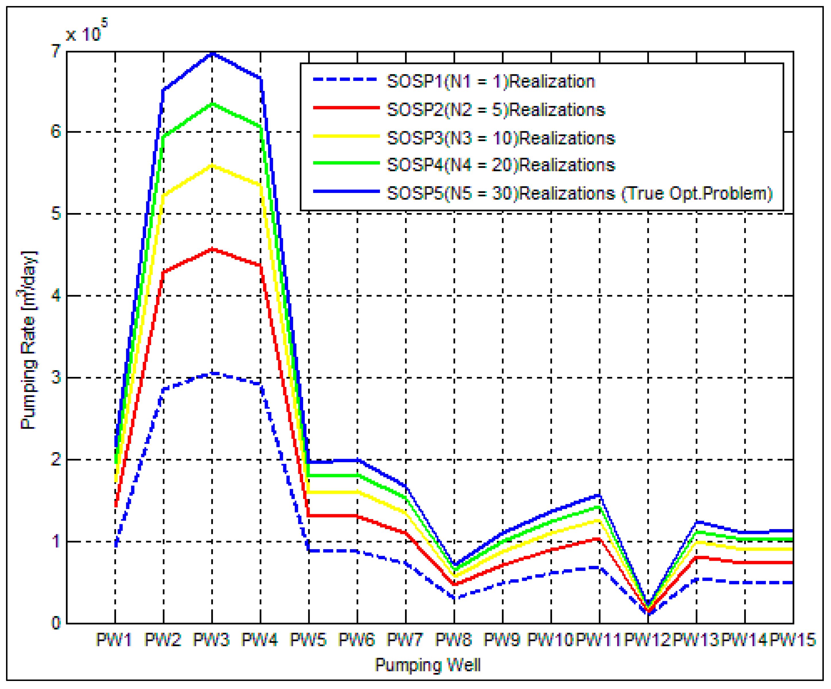
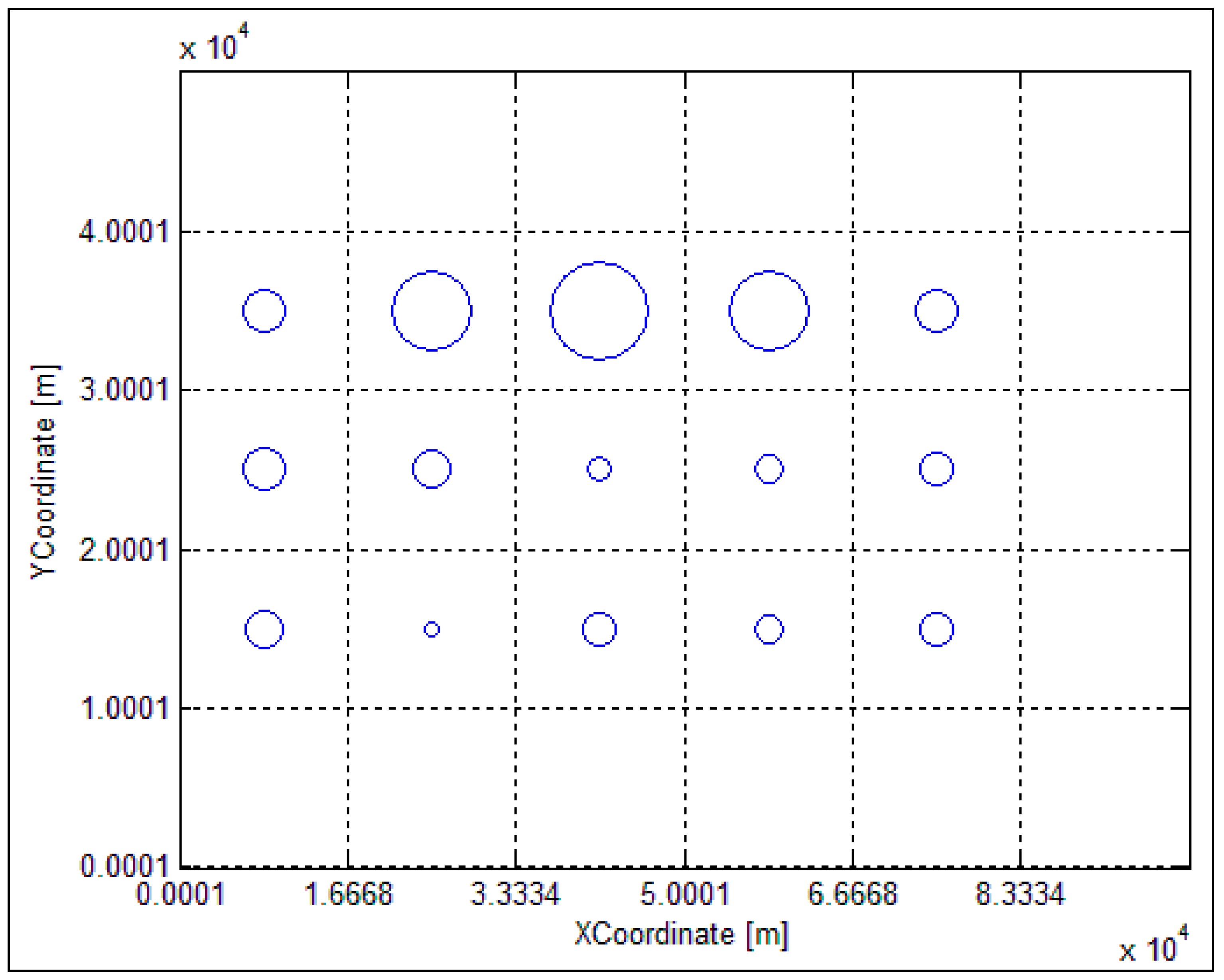
Pumping Well	SOSP1 (N1 = 1) Optimal Pumping Rate (m3/d)	SOSP2 (N2 = 5) Optimal Pumping Rate (m3/d)	SOSP3 (N3 = 10) Optimal Pumping Rate (m3/d)	SOSP4 (N4 = 20) Optimal Pumping Rate (m3/d)	SOSP5 (N5 = 30) Optimal Pumping Rate (m3/d)	50% * Saturated Aquifer Thickness (m) (Maximum Allowable Total Drawdown)
PW1	93,240.00	139,860.00	170,940.00	194,250.00	212,898.00	53.33
PW2	285,480.00	428,220.00	523,380.00	594,750.00	651,846.00	54.27
PW3	305,280.00	457,920.00	559,680.00	636,000.00	697,056.00	51.16
PW4	291,600.00	437,400.00	534,600.00	607,500.00	665,820.00	46.78
PW5	86,040.00	129,060.00	157,740.00	179,250.00	196,458.00	59.38
PW6	87,120.00	130,680.00	159,720.00	181,500.00	198,924.00	56.09
PW7	72,720.00	109,080.00	133,320.00	151,500.00	166,044.00	50.41
PW8	30,600.00	45,900.00	56,100.00	63,750.00	69,870.00	47.06
PW9	47,520.00	71,280.00	87,120.00	99,000.00	118,504.00	49.82
PW10	59,400.00	89,100.00	108,900.00	123,750.00	135,630.00	54.93
PW11	68,400.00	102,600.00	125,400.00	142,500.00	156,180.00	67.61
PW12	9000.00	13,500.00	16,500.00	18,750.00	20,550.00	63.68
PW13	54,000.00	81,000.00	99,000.00	112,500.00	123,300.00	56.45
PW14	48,240.00	72,360.00	88,440.00	100,500.00	110,148.00	53.86
PW15	50,040.00	75,060.00	91,740.00	104,250.00	114,258.00	59.10
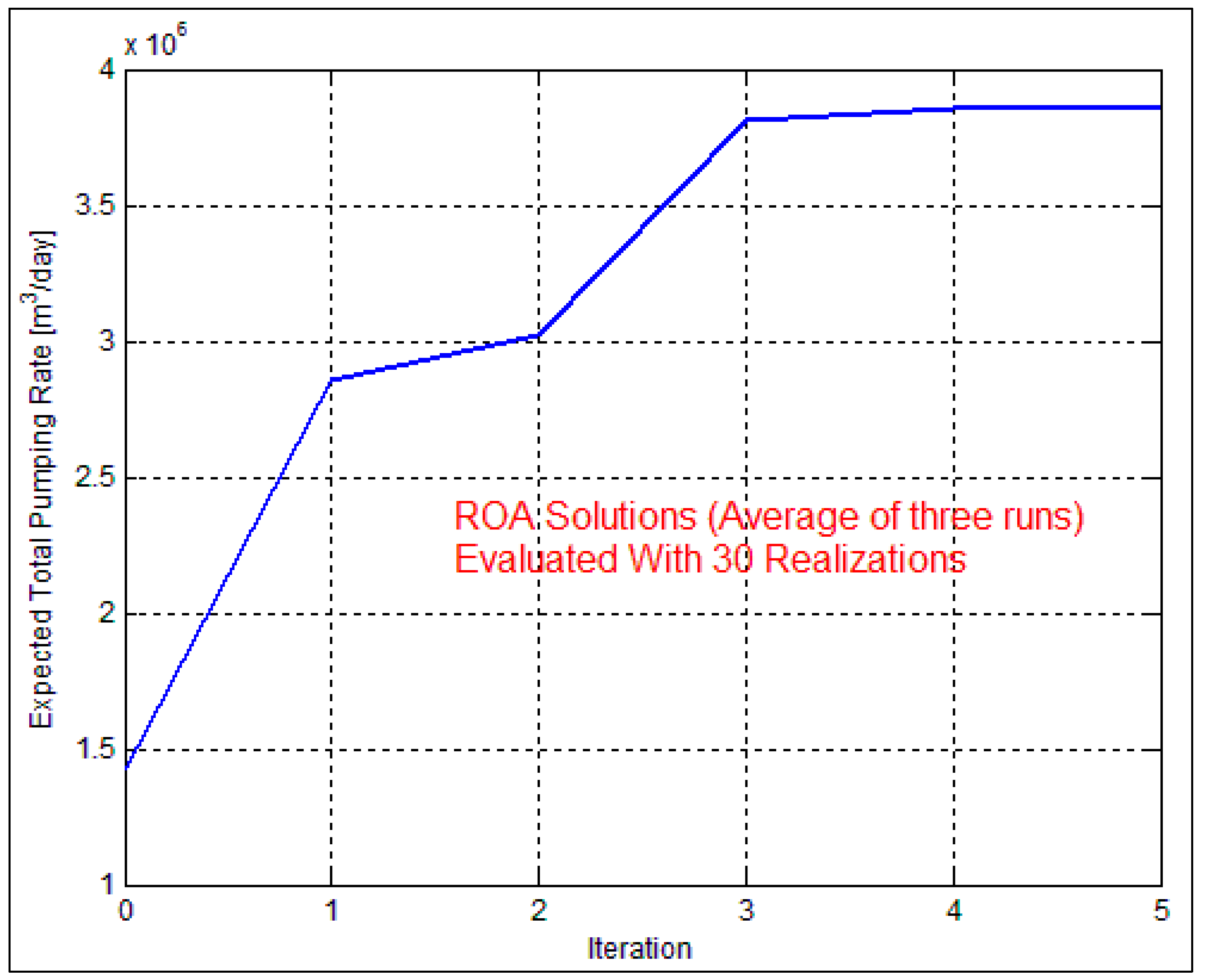
∑	1,588,680.00	2,383,020.00	2,912,580.00	3,309,750.00	3,727,486.00

* Saturated aquifer thicknesses adopted after [23].

presents groundwater pumping rate solution strategies of the five (5) sample path optimization sub-problems with corresponding maximum allowable total drawdowns.

In Table 3, the optimal solution strategies corresponding to the sequence of sample path optimization sub-problems generated yields optimal pumping solutions ranging from a minimum of 9000.00 m³/day to a maximum of 697,056.00 m³/day with optimal objective function values ranging from about a minimum of 1,588,680.00 m³/day to a maximum of 3,727,486.00 m³/day. Figure 5 shows a graph presenting groundwater pumping solutions of the five (5) sample path optimization sub-problems.

As can be seen in Figure 5, the sample path optimization sub-problems optimal solutions converge towards the true groundwater optimization optimum solution as the sample size increases. It should be noted that the first sample path optimization problem (SOSP1) is inexpensive because computing every optimal solution or objective function requires only one function evaluation. The fourth optimal solution (SOSP4) is very close to the true optimization problem (SOSP5) optimal solution. The fifth sample path optimization problem (SOSP5) whereby all the 30 realizations generated were considered converged with a relatively few number of iterations because its initial solution guess (i.e., SOSP4 solution) is nearly equal to the true optimization problem (SOSP5) optimal solution.

The optimization problems were solved with different initial solution guesses for three runs, which resulted in different optimal solutions and, therefore, different objective function values (i.e., different expected total groundwater pumping rates). The results for the expected total pumping rates evaluated over 30 realizations for three runs were then averaged. Figure 6 presents the performance of the ROA framework with cluster sampling for the hypothetical example evaluated over 30 realizations.

In Figure 6, the ROA expected total pumping rate (average of three runs) converged to its maximum value of about 3.7 × 10⁶ m³/day within 3 to 5 iterations (evaluated over the 30 realizations of hydraulic conductivity fields). Figure 7 presents the optimized pumping rates strategy in 2-dimension view via a bubble chart.

In Figure 7, the size of the bubble circles indicates the magnitude of the groundwater pumping rates. Thus, the biggest bubble circle indicates the groundwater well of the highest pumping rate magnitude, and vice versa. Pumping well PW3 and PW12 (see Figure 2) have the maximum and minimum groundwater pumping rates, respectively (see Table 3). The high difference in pumping rate is due to high variation in groundwater (aquifer) recharge opportunity as well as variations in aquifer hydraulic conductivity properties (see Figure 1 and Figure 2). Pumping well PW3 is closer to the river course compared to pumping well PW12 (refer to Figure 2) which is located far from the river course. Pumping well PW3 may receive additional recharge from the river compared to pumping wells which are relatively far from the river. Higher pumping rates are also reflected in pumping wells PW2 and PW4 which are also closer to the river course. Aquifer recharge contributes to aquifer storage as well as to the groundwater pumping yield. It should be noted that even though pumping wells PW1, PW5, and PW6 are closer to the river course, their pumping rates are relatively low compared to those of pumping wells PW2, PW3, and PW4. This is due to variations in water table elevations, hydraulic conductivity properties, and boundary conditions (refer Figure 1 and Figure 2). Pumping wells PW1 and PW6 are closer to a no-flow boundary; hence, high pumping rates would imply a violation of drawdown constraints.

4. Conclusions and Recommendations

In this paper, we introduced a new approach (within the context of groundwater resource management), ROA, applied through a hypothetical aquifer water system, for managing groundwater resources under geological (hydraulic conductivity field) uncertainty. The ROA framework can be used with any underlying optimization algorithm in either stochastic or deterministic core optimizers. We used a deterministic (Active Set algorithm SQP—based gradient search) core optimizer. ROA optimizes by using a sequence of increasing numbers of realizations, and we adopted a k-means clustering sampling technique for realizations selection. By using k-means clustering sampling the ROA–Active Set procedure was able to find a (nearly) converged solution within a relatively few number of iterations, within three to five iterations. In conclusion, our results demonstrate that the ROA approach is a promising technique for use in managing groundwater resources under geological uncertainty. Future research should be focused toward the establishment of guidelines for the determination of the sequence of sample sizes to be used in ROA, use of parallel computer processors, determination of the weights to be used in computing the estimates objective functions, application of the approach for multi-objective optimization, and testing of the overall performance of the optimization procedure.

References

- Tian, J.; Li, C.; Liu, J.; Yu, F.; Cheng, S.; Zhao, N.; Jaafar, W.Z.W. Groundwater Depth Prediction Using Data-Driven Models with the Assistance of Gamma Test. Sustainability 2016, 8, 1076. [Google Scholar] [CrossRef]
- Lee, Y.; Tung, C.; Lee, P.; Lin, S. Personal Water Footprint in Taiwan: A Case Study of Yunlin County. Sustainability 2016, 8, 1112. [Google Scholar] [CrossRef]
- Ndambuki, J.M. Multi-Objective Groundwater Quantity Management: A Stochastic Approach; DUP Science, Delft University Press: Delft, The Netherlands, 2001. [Google Scholar]
- Gelhar, L.W. Stochastic Subsurface hydrology: From Theory to Application. Water Resour. Res. 1986, 22, 135S–145S. [Google Scholar] [CrossRef]
- Safavi, H.R.; Bahreini, G.R. Conjunctive Simulation of Surface Water and Groundwater Resources under Uncertainty. Iran. J. Sci. Technol. Trans. B Eng. 2009, 33, 79–94. [Google Scholar]
- Gorelick, S.M. A Review of Distributed Parameter Groundwater Management Modeling Methods. Water Resour. Res. 1983, 19, 305–319. [Google Scholar] [CrossRef]
- Aguado, E.; Remson, I. Groundwater hydraulics in Aquifer Management. J. Hydrol. Division ASCE 1974, 100, 103–118. [Google Scholar]
- Peralta, R.C.; Azarmnia, H.; Takahashi, S. Embedding and Response Matrix Techniques for Maximizing Steady—State Groundwater Extraction: Computational Comparison. Groundw. J. 1991, 29, 357–364. [Google Scholar] [CrossRef]
- Wang, H.; Ciaurri, D.E.; Durlofsky, L.J.; Cominelli, A. Optimal Well Placement under Uncertainty Using a Retrospective Optimization Framework. SPE J. 2012, 17, 112–121. [Google Scholar] [CrossRef]
- Gorelick, S.M. A Model for Managing Sources of Groundwater Pollution. Water Resour. Res. 1982, 18, 773–781. [Google Scholar] [CrossRef]
- Aguado, E.; Sitar, N.; Remson, I. Sensitivity Analysis in Aquifer Studies. Water Resour. Res. 1977, 13, 733–737. [Google Scholar] [CrossRef]
- Bredehoeft, J.D.; Young, R.A. Conjunctive Use of Groundwater and Surface water for irrigated Agriculture: Risk Aversion. Water Resour. Res. 1983, 19, 1111–1121. [Google Scholar] [CrossRef]
- Mulvey, J.M.; Venderbei, R.J.; Zenios, S.A. Robust Optimisation of Large Scale Systems. Oper. Res. 1995, 43, 264–281. [Google Scholar] [CrossRef]
- Ndambuki, J.M.; Otieno, F.A.O.; Stroet, C.B.M.; Veling, E.J.M. Groundwater Management under Uncertainty: A Multi-Objective Approach. Water SA 2000, 26, 35–42. [Google Scholar]
- Özdogan, U.; Horne, R.N. Optimization of Well Placement under Time-Dependent Uncertainty. SPE Res. Eval. Eng. 2006, 9, 135–145. [Google Scholar] [CrossRef]
- Güyagüler, B.; Home, R.N. Uncertainty Assessment of Well Placement Optimization. SPE Res. Eval. Eng. 2004, 7, 24–32. [Google Scholar] [CrossRef]
- Onwunalu, J.E.; Durlofsky, L.J. Application of a particle swarm optimization algorithm for determining optimum well location and type. Comput. Geosci. 2010, 14, 183–198. [Google Scholar] [CrossRef]
- Yeten, B.; Durlofsky, L.J.; Aziz, K. Optimization of Nonconventional Well Type, Location, and Trajectory. SPE J. 2003, 8, 200–210. [Google Scholar] [CrossRef]
- Chen, Y.; Oliver, D.S.; Zhang, D. Efficient Ensemble-Based Closed-Loop Production Optimization. SPE J. 2009, 14, 634–645. [Google Scholar] [CrossRef]
- Wang, C.; Li, G.; Reynolds, A.C. Production Optimization in Closed-Loop Reservoir Management. SPE J. 2009, 14, 506–523. [Google Scholar] [CrossRef]
- Wang, H.G.; Schmeiser, B.W. Discrete stochastic optimization using linear interpolation. In Proceedings of the 2008 Winter Simulation Conference, Miami, FL, USA, 7–10 December 2008; Mason, S.J., Hill, R.R., Monch, L., Rose, O., Jefferson, T., Fowler, J.W., Eds.; IEEE Press: Piscataway, NJ, USA, 2008; pp. 502–508. [Google Scholar]
- Chen, H.; Schmeiser, B.W. Stochastic root finding via retrospective approximation. IIE Trans. 2001, 33, 259–275. [Google Scholar] [CrossRef]
- Tyagi, N.K.; Srinivaslu, A.; Kumar, A.; Tyagi, K.C. Modelling Conjunctive Use of Water Resources: Hydraulic and Economic Optimization. Available online: http://krishikosh.egranth.ac.in/bitstream/1/2046491/1/CSSRI201.pdf (accessed on 28 June 2016).
- Van Leeuwen, M.; te Stroet, C.B.M.; Butler, A.P.; Tompkins, J.A. Stochastic Determination of Well Capture Zones. Water Resour. Res. 1998, 34, 2215–2223. [Google Scholar] [CrossRef]
- Wagner, J.M.; Shamir, U.; Marks, D.H. Containing Groundwater Contamination: Planning Models using Stochastic Programming with Recourse. Eur. J. Oper. Res. 1994, 77, 1–26. [Google Scholar] [CrossRef]
- Wagner, J.M.; Gorelick, S.M. Reliable Aquifer Remediation in the Precence of Spartially Variable Hydraulic Conductivity: From Data to Design. Water Resour. Res. 1989, 25, 2211–2225. [Google Scholar] [CrossRef]
- Wagner, J.M.; Shamir, U.; Nemati, H.R. Groundwater Quality Management under Uncertainty: Stochastic Programming Approaches and the Value of Information. Water Resour. Res. 1992, 28, 1233–1246. [Google Scholar] [CrossRef]
- Harbaugh, A.W.; Banta, E.R.; Hill, M.C.; McDonald, M.G. MODFLOW-2000, the U.S. Geological Survey Modular Ground-Water Model—User Guide to Modularization Concepts and the Ground-Water Flow Process; OFR: Reston, Virginia, USA, 2000; p. 127. [Google Scholar]