Moving Low-Carbon Transportation in Xinjiang: Evidence from STIRPAT and Rigid Regression Models

Abstract

With the rapid economic development of the Xinjiang Uygur Autonomous Region, the area’s transport sector has witnessed significant growth, which in turn has led to a large increase in carbon dioxide emissions. As such, calculating of the carbon footprint of Xinjiang’s transportation sector and probing the driving factors of carbon dioxide emissions are of great significance to the region’s energy conservation and environmental protection. This paper provides an account of the growth in the carbon emissions of Xinjiang’s transportation sector during the period from 1989 to 2012. We also analyze the transportation sector’s trends and historical evolution. Combined with the STIRPAT (Stochastic Impacts by Regression on Population, Affluence and Technology) model and ridge regression, this study further quantitatively analyzes the factors that influence the carbon emissions of Xinjiang’s transportation sector. The results indicate the following: (1) the total carbon emissions and per capita carbon emissions of Xinjiang’s transportation sector both continued to rise rapidly during this period; their average annual growth rates were 10.8% and 9.1%, respectively; (2) the carbon emissions of the transportation sector come mainly from the consumption of diesel and gasoline, which accounted for an average of 36.2% and 2.6% of carbon emissions, respectively; in addition, the overall carbon emission intensity of the transportation sector showed an “S”-pattern trend within the study period; (3) population density plays a dominant role in increasing carbon dioxide emissions. Population is then followed by per capita GDP and, finally, energy intensity. Cargo turnover has a more significant potential impact on and role in emission reduction than do private vehicles. This is because road freight is the primary form of transportation used across Xinjiang, and this form of transportation has low energy efficiency. These findings have important implications for future efforts to reduce the growth of transportation-based carbon dioxide emissions in Xinjiang and for any effort to construct low-carbon and sustainable environments.

1. Introduction

The CO₂ emissions generated by human activities constitute one of the most significant contributory factors to global warming. As pointed out by the IPCC in its fifth assessment report, of the total global greenhouse gas emissions in 2014, urban transportation accounted for 13.1%. This made urban transportation the third highest emission sector, behind only energy supply and industrial production [1]. In 2010, the petroleum consumption of the transportation sector accounted for 38.25% of China’s total petroleum consumption. This substantial consumption of petroleum resulted in the continuing increase of CO₂ emissions [2,3]. Located in the northwest border area of China, Xinjiang Uygur Autonomous Region is China’s largest provincial-level administrative region, and major energy supply base. Moreover, this region is home to ethnic minorities, such as Uighur and Kazaks. In addition, Xinjiang is also an important channel for economic exchanges between China and Central Asia. Since the implementation of the Western Development Strategy in 2001 and the Jumping Development Strategy in 2010 [4], Xinjiang’s transportation sector has witnessed rapid and sustained development. The total output value of the transportation sector increased from USD 305.8 million in 1990 to USD 748.5 million in 2012. This represented an average annual growth rate of 14.9%. During the same period, the energy consumption of the transportation sector also experienced a rapid rise, from 10.71 million tons of standard coal to an amazing 85.54 million tons of standard coal. This translates to an average annual growth rate of 9.5% [5]. Accompanied by the substantial consumption of energy, CO₂ emissions also inevitably increased at a rapid rate. In 2013, the Chinese government put forward the One Belt, One Road Initiative [6]. By virtue of its unique geographic location, Xinjiang will undoubtedly see a rapid development of its transportation sector after the implementation of this initiative [7]. In the short term, the development of the transportation sector will inevitably give rise to even more carbon emissions. Consequently, accurate monitoring and accounting of the transportation sector’s carbon emissions and a quantitative analysis of those factors that influence carbon emissions will provide important policy implications for the green and low-carbon development of transportation in Xinjiang.

With the continuous advance of economic globalization, the energy consumption of the transportation sector has received growing attention. As a key component of sustainable development, reducing the level of energy use in the transportation sector would both tackle energy security and address climate change concerns [8,9,10,11,12,13,14,15,16,17,18,19]. Researchers have analyzed the carbon emissions of the transportation sector from various perspectives. Several studies have made creditable attempts to accurately calculate transportation-related carbon emissions and build models of the influencing factors [20,21,22,23,24,25,26,27,28,29,30,31,32,33,34,35,36,37]. Chandran et al. [25] introduced a co-integration analysis and Granger causality analysis to study the influence of energy-related CO₂ emissions in the transportation sector on five Association of Southeast Asian Nations (ASEAN) countries. The results indicated that reducing the energy consumption of the transportation sector would undoubtedly reduce carbon emissions in the short term. However, in the long run, the most fundamental way to reduce carbon emissions is to improve the transportation sector’s efficiency in terms of energy utilization and to optimize energy structures. Saboori et al. [22] adopted the “fully modified ordinary least square method” (FMOLS) and generalized impulse response to explore the relationships between energy consumption in the road transport sector, CO₂ emissions and the economic growth in Organization for Economic Co-operation and Development (OECD) countries. The results indicated the existence of a positive, significant, long-run and bi-directional relationship between CO₂ emissions and economic growth, road sector energy consumption and economic growth and CO₂ emissions and road sector energy consumption in all OECD countries. Moreover, in most cases, any effort on carbon emissions caused by changes in the road transport sector’s energy consumption lasts longer than effects brought about due to economic growth. In addition, many scholars have also studied the CO₂ reduction potential in the transport sector at the national level [2,33,38,39,40,41,42,43,44,45,46,47,48,49,50]. For instance, Xu et al. [46,51] introduced the vector auto-regression model and the dynamic non-parametric additive regression model as a means to analyze the factors that influenced the CO₂ emissions of China’s transportation sector. This study concluded that improving energy efficiency will reduce CO₂ emissions, but increasing the total number of private vehicles and promoting the progress of urbanization will significantly increase CO₂ emissions. Ratanavaraha et al. [29] considered five independent variables, namely (1) the size of the population, (2) gross domestic product (GDP) and the number of (3) small, (4) medium and (5) large-sized registered vehicles, and employed four different measurement techniques (log-linear regression, path analysis, time series and curve estimation) to forecast the carbon emissions coming from Thailand’s transportation sector. The researchers claimed that the primary means of reducing carbon emissions will be to improve the energy efficiency of motor vehicles and to transform the current highway freight-based mode of transportation. Shahbaz et al. [52] applied combined co-integration tests and Autoregressive Distributed Lag (ARDL) bound tests to investigate the causal relationships between transportation-related energy consumption, CO₂ emissions, fuel prices and transport sector added value in Tunisia. The test results indicated that the energy consumption and added value output of the transportation sector promotes CO₂ emissions, but increases in fuel prices reduce the level of CO₂ emissions.

In terms of the content of prior research, all of the studies mentioned above focus on the macro-level (specifically, the international or national level), but research on a local level is rare. Taking China as an example, many studies have been conducted at a national level, but few have addressed the provincial level [33,44,45,46,51]. Given that the carbon emissions of the transportation sector are restrained by many region-specific factors (such as topography and geomorphology, energy endowments and regional energy policies, which differ significantly from region to region), it is necessary to carry out a microscopic analysis. Furthermore, with regard to the research methods, two approaches are widely used at present. They are the index decomposition method [6,7,8,11,20,23,53] and the econometric method [2,4,6,24,28,54,55]. Due to the constraints of the Kaya identity, the factors that are considered in the index decomposition method are limited. There are also defects in the econometric method. In particular, the econometric method usually explores the relationships among variables from the perspectives of co-integration and causality, but neglects the multicollinearity problems, which prevail in macroeconomic data.

Compared with previous studies, this paper fills the above-mentioned gaps in the following three ways: Firstly, our research empirically studies the carbon emissions of the transport sector at the local level, while at the same time taking into consideration each local area’s significant uniqueness. Xinjiang is China’s largest provincial-level administrative region, with an area of approximately 1.66 million km². The region accounts for one-sixth of China’s total land area. Remarkably, transportation in Xinjiang is mainly based on road freight. Moreover, the One Road, One Belt Initiative [6] aims to promote communication and cooperation between the countries along the Silk Road. The initiative also aims to promote the construction of transportation infrastructure in Xinjiang, which will in turn result in a rapid rise in transportation-related carbon emissions. Secondly, in terms of methodology, the STIRPAT (Stochastic Impacts by Regression on Population, Affluence and Technology) model and the ridge regression model were combined in this paper to thoroughly analyze the influencing factors of carbon emissions. Our approach effectively overcomes the multicollinearity problem inherent in macroeconomic variables and, thus, guarantees the objectivity and reliability of our estimated results. Finally, the accounting of the carbon emissions of the transportation sector in this study is both comprehensive and accurate. Specially, our study respectively calculates the carbon emissions from nine types of energy, namely coal, coke, crude oil, gasoline, kerosene, diesel, fuel oil, natural gas and electricity. Thus, the results of our study better reflect Xinjiang’s conditions and are more scientific.

2. Methodology and Data

2.1. Accounting of Carbon Emissions

Currently, two methods are primarily used for the accounting of the carbon emissions of the transportation sector, namely the “bottom-up distance-based” method and the “top-down fuel-based” method [56]. The former method calculates the total carbon emissions according to the vehicle mileage of the various means of transportation, as well as the energy consumption per unit of mileage and the carbon emission coefficients of the various types of energies in the region studied. The latter method calculates the total carbon emissions by multiplying the energy consumption of the transportation sector by the carbon emission coefficients of various energy types. Considering the difficulty of fully and reliably collecting the mileage data of different vehicle models, as required by the “bottom-up distance-based” method, this paper adopted the “top-down fuel-based” method to calculate the CO₂ emissions of Xinjiang’s transportation sector. The calculation formula is as follows:

$$C={\displaystyle \sum _{i=0}^n{C}_i}={\displaystyle \sum _{i=0}^n{E}_i}\times LC{V}_i\times PC{C}_i\times O_i\times 44/12$$

(1)

where $C$ represents the total CO₂ emissions of the energy consumption of the transportation sector; $C_i$ denotes the CO₂ emissions based on fuel type $i$; $E_i$ is the consumption of fuel type $i$; $LC{V}_i$ and $PC{C}_i$ represent the low calorific value and the potential carbon content of fuel type $i$, respectively; $O_i$ represents the oxidation rate of fuel type $i$; $44/12$ is the coefficient of conversion from $C$ to CO₂. See the CO₂ emissions factors of the various energy types in

Table 1. CO₂ emission factors of various energy types.

Fuel Type	Coal	Coke	Crude Oil	Gasoline	Kerosene	Diesel Oil	Fuel Oil	Natural Gas
Low calorific value (TJ/103 t or TJ/104 m3) [59]	20.908	28.435	41.816	43.070	43.070	42.652	41.816	38.93
Potential carbon content (kg C/GJ) [60]	26.37	29.5	20.1	18.9	19.6	20.2	21.1	15.3
Oxidation rate [60]	0.98	0.93	0.98	0.98	0.98	0.98	0.98	0.99

. Based on the baseline emissions factor of the power grid in northwest China and the related literature [57,58], the CO₂ emissions factor of electricity in Xinjiang was determined as being 1.0174 tCO₂/MWh.

2.2. STIRPAT (Stochastic Impacts by Regression on Population, Affluence and Technology) Model

The STIRPAT model was proposed by Dietz and Rosa [61]. It was extended on the basis of the IPAT (Impact = Population × Affluence × Technology) model, which was put forward by Ehrlich and Holden [62]. The STIRPAT model has overcome the limitations of IAPT’s hypothesis that “various factors influence the environment by the same proportion” [54]. The STIRPAT model can also better reflect the non-monotonic or non-proportional functional relationships between the factors that influence the natural environment [54,55,63]. The STIRPAT model is as follows:

$$I_t=a{P_t}^b{A_t}^c{T_t}^d{e}_t$$

(2)

where $I$ represents the environmental influence; $P$ represents the population size; $A$ represents the wealth level, generally measured by per capita GDP; $T$ is the technical index, usually measured by the effect on the environment per output; $a$, $b$, $c$ and $d$ represent the model coefficients to be estimated; $e_t$ represents the random error term. The subscript $t$ denotes the time, which usually is the corresponding year. The STIRPAT model combines economic activities and environmental influence and is widely applied as a means to analyze factors influencing the environment. In order to eliminate the heteroscedasticity, which could possibly exist in the model, as well as to facilitate the testing of hypotheses, all of the factors take a logarithmic form. Because $e_t$ is the random error term, we do not need to distinguish between $e_t$ and $L{e}_t$. Then, we rewrote Equation (2) as follows:

$$Ln{I}_t=Lna+bLn{P}_t+cLn{A}_t+dLn{T}_t+e_t$$

(3)

where $P$, $A$ and $T$ are the same as in Equation (2). In order to probe the influencing factors of the transport sector’s CO₂ emissions, we use the total transport-related CO₂ emissions to represent the environmental influence. Equation (3) can then be rewritten as follows:

$$LnC{O}_{2t}=a+{\mathsf{\beta }}_{1}Ln{P}_t+{\mathsf{\beta }}_{2}Ln{A}_t+{\mathsf{\beta }}_{3}Ln{T}_t+e_t$$

(4)

where $C{O}_2$ represents the total $C{O}_2$ emissions of the transportation industry (10⁴ t), and this implies environmental impact; $P$ represents the population size (10⁴ persons); $A$ represents the economic development level, which is expressed in this paper by per capita GDP (10⁴ yuan/person, converted by 1990 as the constant price level); $T$ represents the energy intensity, that is the ratio of total energy consumption to the added value output of the transportation sector (tce/10⁴ yuan). Herein, total energy consumption refers to the sum of the main nine types of energy, which had been converted to tons of standard coal equivalent (tce), respectively.

To further analyze the driving forces of the transport sector’s CO₂ emissions and considering the specific situation in Xinjiang, we expand Equation (4) by incorporating CT (Cargo Turnover) and PC (Private Vehicle Population) into the model. There are two main reasons for incorporating these two variables. On the one hand, Xinjiang is a vast territory, with great distances between cities. Moreover, the main mode of transport in Xinjiang is road freight, which relies chiefly on heavy lorries. The extensive use of heavy lorries means higher energy consumption and higher carbon emissions. Therefore, cargo turnover is an important factor affecting the carbon emissions from the transport sector. On the other hand, due to the increase in residents’ incomes in recent years, the demand for private vehicles continues to rise. The rapid growth in private vehicle ownership has resulted in the corresponding and continued increase in energy consumption and, in turn, energy-related CO₂ emissions. Thus, cargo turnover and private vehicles were incorporated into the estimated model.

Based on the STIRPAT model and the above analysis, the econometric model of the transport sector’s CO₂ emissions is established as follows:

$$LnC{O}_{2t}=a+{\mathsf{\beta }}_{1}Ln{P}_t+{\mathsf{\beta }}_{2}Ln{A}_t+{\mathsf{\beta }}_{3}Ln{T}_t+{\mathsf{\beta }}_{4}LnC{T}_t+{\mathsf{\beta }}_{5}LnP{C}_t+e_t$$

(5)

where $C{O}_2$, $P$, $A$ and $T$ are the same as in Equation (4). CT denotes cargo turnover (100 million ton-km), and PC represents private vehicle population (by unit); ${\mathsf{\beta }}_1$, ${\mathsf{\beta }}_2$, ${\mathsf{\beta }}_3$, ${\mathsf{\beta }}_4$ and ${\mathsf{\beta }}_5$, respectively, represent the elasticity coefficients of the various variables corresponding to $C{O}_2$ emissions.

2.3. Multicollinearity Diagnostics and Ridge Regression

Multicollinearity is a phenomenon in which two or more predictor variables in a multiple regression model are highly correlated. This means that one variable can be linearly predicted from the others with a substantial degree of accuracy [64,65]. In this situation, the coefficient estimates of the multiple regression may change erratically in response to small changes in either the model or the data. Multicollinearity affects calculations regarding individual predictors [66]. That is, a multiple regression model with correlated predictors may not give valid results pertaining to any individual predictor, or about which predictors are redundant with respect to others. To determine whether or not there was multicollinearity existing between independent variables, a multivariate linear regression analysis using least squares was conducted. If the Variance Inflation Factor (VIF) of independent variables was greater than the maximum tolerance of 10, this indicates the existence of multicollinearity between explanatory variables [66,67,68]. A multiple regression model can be expressed as follows:

$$Y=X\mathsf{\beta }+\mathsf{\epsilon }$$

(6)

where $Y$ is an $n\times 1$ observation vector; $X={\left[x_1,x_2,\mathrm{...},x_n\right]}^{\mathrm{T}}$ is an $n\times q$ full rank matrix; $\mathsf{\beta }={\left[{\mathsf{\beta }}_1,{\mathsf{\beta }}_2,\mathrm{...},{\mathsf{\beta }}_q\right]}^{\mathrm{T}}$ is a $q\times 1$ parameter vector to be estimated. By using the least square method, the estimated value of $\mathsf{\beta }$ can be obtained from Equation (7). The mean square error of $\widehat{\mathsf{\beta }}$ is calculated by Equation (8); wherein ${\mathsf{\lambda }}_i$ is $q$ the characteristic root of the non-negative symmetric matrix $X^{\mathrm{T}}X$.

$$\widehat{\mathsf{\beta }}=\left(X^{\mathrm{T}}X\right)X^{\mathrm{T}}Y$$

(7)

$${\widehat{\mathsf{\beta }}}_{MSK}=E\left|{\Vert \widehat{\mathsf{\beta }}-\mathsf{\beta }\Vert }^2\right|=E\left|{\left(\widehat{\mathsf{\beta }}-\mathsf{\beta }\right)}^{\mathrm{T}}.\left(\widehat{\mathsf{\beta }}-\mathsf{\beta }\right)\right|={\mathsf{\sigma }}^2{\displaystyle \sum _{i=1}^q\frac{1}{{\mathsf{\lambda }}_i}}$$

(8)

When multicollinearity existed between independent variables, the matrix $X^{\mathrm{T}}X$ is singular, and some of the matrix’s characteristic roots are close to zero. Under these conditions, the value of ${\widehat{\mathsf{\beta }}}_{MSK}$ will be especially large, which indicates a larger deviation between the estimated values and observed values. Thus, the ordinary least squares (OLS) method loses its stability and reliability. Ridge estimation (RE) is an alternative method to the OLS method and can be used when a collinearity problem exists in a linear regression model [64,65,66,67].

To address the aforementioned problem, the ridge regression method substitutes $X^{\mathrm{T}}X$ for $X^{\mathrm{T}}X+kI$ to ensure the characteristic roots of matrix $X^{\mathrm{T}}X+kI$ are far from zero. Then, the value of ${\widehat{\mathsf{\beta }}}_{MSK}$ will be significantly reduced. Finally, the estimated value of $\mathsf{\beta }$ can be solved by Equation (9).

$$\widehat{\mathsf{\beta }}(k)={\left(X^{\mathrm{T}}X+kI\right)}^{-1}{X}^{\mathrm{T}}Y$$

(9)

Herein, $I$ is an identity matrix, $k$ is a ridge parameter and $\widehat{\mathsf{\beta }}(k)$ is the ridge estimated value for $\mathsf{\beta }$. In this paper, we determined the ridge parameters by means of the ridge trace method.

2.4. Data Sources and Description

The data used in this paper include annual observations of the CO₂ emissions, population size, per capita GDP, energy intensity, cargo turnover and private vehicle population in Xinjiang during the period from 1990 to 2014. In order to eliminate the effect of price changes, per capita GDP is calculated at a constant price (1990 = 100). All data used in this paper are obtained from 50 Years of Glories of Xinjiang [69], the Xinjiang Statistical Yearbook (XSY) (1989 to 2014) [5] and the China Energy Statistical Yearbook (1990 to 2014) [70]. Data on the level of energy consumption of the various types of energy used by the transport sector were derived from the table of “Energy Consumption by Sector and Major Energy Consumption” provided by the Xinjiang Statistical Yearbook [5]. Total energy consumption data came from the China Energy Statistical Yearbook [70]. The data relating to GDP, population size, total number of private vehicles, cargo turnover and transportation sector’s added value output came from the 50 Years of Glories of Xinjiang and the Xinjiang Statistical Yearbook [5]. In order to eliminate the effects of inflation, GDP is again calculated at a constant price (1990 = 100). Cargo turnover represents total freight ton-kilometers, which included four categories, namely railways, highways, civil aviation and petroleum and gas pipelines. It is calculated as being transport mileage multiplied by freight volume. In view of the classification standards of the National Bureau of Statistics, there are two types of private cars, namely passenger cars and freight cars. Moreover, passenger cars are divided into four sub-categories: large, medium, small and micro cars. Freight car categories include heavy, medium, light and miniature. Private car ownership in this paper is calculated as the total amount of the above-mentioned types of motor vehicles.

3. Results and Discussion

3.1. Features of Carbon Emissions from the Transport Sector

3.1.1. Macro-Level: Total Energy-Related Carbon Emissions

The estimated results of the total carbon emissions and per capita carbon emissions of Xinjiang’s transportation sector during the period of from 1989 to 2012 are shown in Figure 1. As shown, on the whole, the two indicators display a gradually rising trend. Based on the changes in trend, the study period could be divided into two phases: 1989 to 2000 and 2001 to 2012. In the first phase, both the total carbon emissions and per capita carbon emissions presented a slowly rising trend with their average annual growth rates of 6.8% and 4.5%, respectively. In the second phase, the total carbon emissions increased from 5.35 million tons to 16.53 million tons. This represented a total growth of 310% over the duration of the period and an average annual growth rate of 10.8%. During the same phase, the per capita carbon emissions increased from 0.29 t to 0.74 t, or a total growth of 260% and an average annual growth rate of 9.1%. The enormous differences between the two phases in terms of growth rate can be explained by the implementation by the central government of the Western Development Strategy in 2001 [4]. The implementation of this strategy has promoted the construction of transportation infrastructure and thus facilitated the development of the logistics sector. With the rapid development of the logistics sector, the carbon emissions caused by energy consumption have also increased.

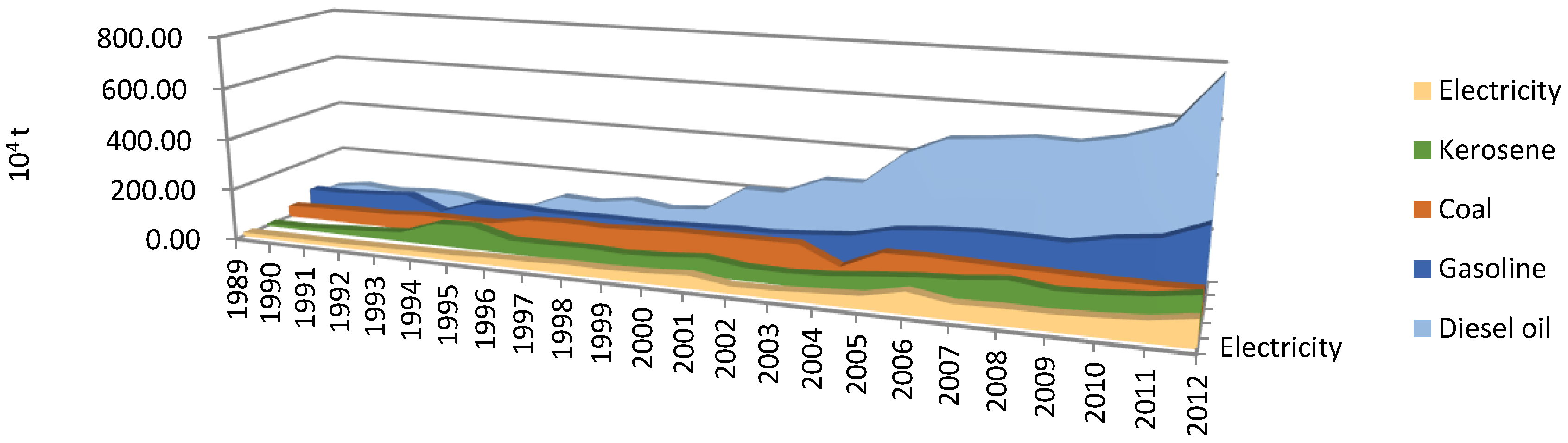
3.1.2. Micro-Level: Carbon Emissions Structure and Intensity

The structure of carbon emissions can be analyzed from different aspects. Due to the fact that energy mix has an important influence on carbon emissions, energy mix thus became the most commonly-used means to illustrate the changes of the carbon emissions structure. Figure 2 shows the CO₂ emissions from the five major energy types during the period from 1989 to 2012. Three interesting results can be drawn from this figure. Firstly, as a whole, the level of carbon emissions from all fuel types continued to increase during the study period, especially since 2004. According to XSY [5], the length of road transport lines has increased markedly since 2004, which in turn indicates that the construction of traffic facilities can lead to a rapid growth in energy consumption (for transportation). Secondly, diesel oil, rather than gasoline, turns out to be the biggest emitter of carbon emissions. In the period from 1989 to 2012, the highest carbon emissions were generated by the consumption of diesel oil, with an average value of 2.60 million tons per year and a proportion as high as 36.2% of all emissions. Thirdly, the use of cleaner energies such as electricity experienced steady growth. However, clean energy still only accounts for a very small slice of the total energy “pie”, with an average annual value of 0.42 million tons, representing only 7.1% of usage among all fuel types. However, it should be noted that, since 2012, almost half a million cars and buses and more than 100,000 private cars in Xinjiang have been using Liquid Natural Gas (LNG) for eco-friendliness and higher efficiency purposes. The use of LNG is potentially a fundamental way to reduce CO₂ emissions in Xinjiang. At present, there are three types of railway locomotives in Xinjiang, which are steam locomotives, diesel locomotives and electric locomotives. Steam locomotives use coal as the driving energy. For example, in Sandaoling coal mine, which is located in Hami Prefecture, the steam locomotive still bears the task of coal transportation. However, it should be noted that the coal consumption in the transport sector is gradually decreasing. As for kerosene, it is mainly used in air transport. Because there is great distance from one city to another in Xinjiang, travel by air is preferred by more and more people. Therefore, the consumption of kerosene showed a rising trend in the research period.

In addition to the energy mix, we further analyzed the characteristics of traffic carbon emissions in Xinjiang from the perspective of carbon emission intensity. Carbon emission intensity is defined as the amount of carbon dioxide emissions per unit of GDP growth. Herein, for the purpose of this study, both carbon dioxide emissions and GDP are limited to the transport sector. The calculation results of carbon emission intensity are shown in

Table 2. The carbon emission intensity in Xinjiang’s transport sector.

Year	Total Carbon Emissions (104 t)	Value Added Output (104 Yuan)	Emission Intensity (t/104 Yuan)	Year	Total Carbon Emissions (104 t)	Value Added Output (104 Yuan)	Emission Intensity (t/104 Yuan)
1989	199.26	12.90	15.45	2001	535.29	148.38	3.61
1990	225.94	14.63	15.44	2002	496.71	168.58	2.95
1991	233.82	22.63	10.33	2003	572.34	159.43	3.59
1992	266.79	28.32	9.42	2004	596.08	186.70	3.87
1993	234.29	32.58	7.19	2005	800.98	149.61	5.35
1994	304.22	44.40	6.85	2006	934.27	165.60	5.64
1995	317.89	59.63	5.33	2007	936.43	177.28	5.28
1996	366.69	73.74	4.97	2008	1243.52	191.84	6.48
1997	368.48	85.70	4.30	2009	1204.18	209.10	5.76
1998	394.47	106.87	3.69	2010	1249.61	222.47	5.62
1999	372.73	129.60	2.88	2011	1313.75	256.72	5.12
2000	412.93	148.63	2.78	2012	1653.05	357.90	4.62

.

As can be seen from Table 2, the changes in trends were relatively complicated. According to the characteristics of numerical value change, the study period was divided into three phases for the convenience of analysis. In the first phase (1989 to 2000), the intensity of carbon emissions steadily declined, from 15.45 t/10⁴ yuan in 1989 to 2.78 t/10⁴ yuan in 2000 with an average annual rate of decline of 16.9%. This phase corresponded to China’s “Eighth Five-year Plan” and “Ninth Five-year Plan” [71], in which the government’s energy policies focused on the control of energy consumption and improvements in efficiency. These plans and policies were the primary cause of the year-by-year decline in the intensity of carbon emissions [72,73]. In the second phase (2001 to 2008), the intensity of carbon emissions rose, although the degree of increase fluctuated. To be specific, the intensity of carbon emissions reached 6.48 t/10⁴ yuan in 2008. The implementation of the Western Development Strategy [4] and China’s accession to the World Trade Organization (WTO) may be the main causes for this rise. According to XSY [5], during this period, the level of cargo turnover increased sharply, with an annual growth rate of 12.76%. Moreover, the average share of highway use for freight traffic reached as high as 81.0%. A high proportion of highway transport means a corresponding increase in energy consumption. During the third phase (2009 to 2012), the intensity of carbon emissions experienced a declining trend. Along with the economic development of Xinjiang, the government attached greater importance to efficient energy utilization. Meanwhile, the cooperation between China and Central Asia in the field of energy (especially natural gas) accelerated the optimization of the energy consumption structure of Xinjiang’s transportation sector. This optimization, in turn, directly and continuously, reduced the intensity of carbon emissions during this period [3,74,75].

3.2. Multicollinearity Detection and Ridge Regression Analysis

In the presence of multicollinearity, the estimate of one variable’s impact on dependent variable $Y$ while controlling for the others tends to be less precise than if predictors were uncorrelated [76]. Therefore, detecting any multicollinearity before estimating the parameters becomes necessary. First of all, by using the OLS method, we estimated the parameters in the STIRPAT model. Then, in accordance with the VIF, we can determine whether multicollinearity exists between the variables [77]. Finally, one typical remedy for multicollinearity will be adopted in this paper. The results of OLS regression and the VIF values of each variable are listed in

Table 3. The OLS regression results of transport’s carbon emission in Xinjiang.

Variables	Parameters	Standard Error	t Statistics	p-Value	Variance Inflation Factor (VIF)
Constant	−17.152	6.546	−2.620	0.017 **	—
lnP	2.411	0.853	2.837	0.011 **	56.437
lnA	0.498	0.237	2.101	0.050 *	34.681
lnT	0.293	0.065	4.490	0.000 ***	4.649
lnCT	0.105	0.269	0.391	0.700	155.264
lnPC	0.095	0.159	0.601	0.556	226.711

Note: ***, ** and * denote significant level at 1%, 5% and 10%, respectively.

.

As can be seen from Table 3, the VIF values of population size, per capita GDP, cargo turnover and private vehicles were far greater than 10. This finding indicates the existence of multicollinearity between the explanatory variables. Therefore, the OLS method was not suitable for making an unbiased estimation. In order to obtain more accurate results, a ridge regression estimation was used to re-estimate the model in Equation (5). Ridge regression estimation involves an improved algorithm of least squares and can address the previous inability to inversely solve the matrix for the coefficient vector by using least squares [68]. By adding a non-negative factor $K$ to the element on the main diagonal of a standardized matrix of independent variables, the ridge regression algorithm was able to significantly improve the stability of estimation [4]. Since the ridge regression is a biased estimate, to retain as much information as possible, the value of $K$ should not be overly large. The ridge parameter $K$ fell within the range of (0, 1), and the step size of 0.005 was adopted for the purpose of valuation. When k = 0.02, the coefficient of determination $R^2$ was 0.987, and the regression coefficient of each explanatory variable was stabilized. The ridge regression estimation results are listed in

Table 4. Ridge regression estimation results of the carbon emissions of Xinjiang’s transportation sector.

Variables	Parameters	Standard Error	Standardized Coefficients	t Statistics	p-Value
Constant	−12.504	2.207	0.000	−5.665	0.000 ***
P	1.777	0.344	0.358	5.159	0.000 ***
A	0.416	0.127	0.236	3.284	0.004 ***
T	0.261	0.038	0.197	6.831	0.000 ***
CT	0.224	0.055	0.237	4.061	0.001 ***
PC	0.110	0.024	0.238	4.558	0.000 ***
Adjusted R2 = 0.987		F statistics = 360.31		Significance (F statistics) = 0.000 ***

Note: ***, ** and * denote significant level at 1%, 5% and 10%, respectively.

.

As shown in Table 4, the general coefficient of the model’s determination R² was 0.987, with a relatively high degree of fit. Every explanatory variable passed the t-test significantly. Therefore, the regression coefficients were valid. See the specific ridge regression equation below:

$$LnC{O}_2=-12.504+1.777LnP+0.416LnA+0.261LnT+0.224LnCT+0.110LnPC$$

(10)

As shown by the results of ridge regression, population size is the most important driver of the carbon emission increases of Xinjiang’s transportation sector. Specifically, every 1% growth in population size would cause the transportation sector’s carbon emissions to increase by approximately 1.78%. To the best of our knowledge, there are three main reasons for this phenomenon. Firstly, since the implementation of the family planning policy in China, the natural growth rate of the population has gradually declined, year on year [78]. However, due to more liberal childbearing policies for minorities, the population of Xinjiang has grown more rapidly than in other regions. In the study period, the natural growth rate of Xinjiang’s population was approximately 12.48%. This rate is 4.2% higher than the national average, which was only 8.28%. The growth in population inevitably drives the increase of transportation-related energy consumption, which correspondingly elevates the level of CO₂ emissions. Secondly, the rate of population flow (which included the migration from rural areas to the city both within and outside Xinjiang) is growing faster in recent years. According to XSY [5], Xinjiang is currently experiencing a process of rapid urbanization. The urbanization level of Xinjiang increased from 33.8% in 1989 to 44.0% in 2012. It is recognized that urban form features affect the distance people travel each day, as well as their choice of transportation mode and ultimately the level of CO₂ emissions. Thirdly, due to the long distances between the various prefectures and cities in Xinjiang, compared to inland provinces, Xinjiang experiences higher levels of energy consumption and CO₂ emissions as a direct result of population flow.

In addition, the increase in per capita income constitutes another important factor influencing the carbon emissions of Xinjiang’s transportation sector. The elasticity coefficient of transportation-related carbon emissions for per capita GDP is 0.42%. This finding indicates that, with the continuous rise in social and economic development levels, transportation-related carbon emissions are correspondingly gradually increasing. These increases in per capita income and carbon emissions can be interpreted from two aspects. On the one hand, higher incomes cause more people to buy private cars. The increased number of vehicles on the road naturally leads to increased energy consumption, which in turn results in higher CO₂ emissions. On the other hand, the increased per capita income encourages more people to travel. The increased number of people’s trips will also increase energy consumption, which then boosts the level of CO₂ emissions coming from the transport sector.

As indicated by the energy intensity coefficient, for every 1% increase in energy consumption per unit GDP, carbon emissions increase by 0.26%. In other words, energy intensity and carbon emissions are positively correlated. That is, a reduction in energy intensity will effectively decrease the amount of carbon emissions. In the study period of 1989 to 2012, the energy intensity of Xinjiang’s transportation department continuously declined. In turn, these declines contributed to the reduction of carbon emissions. However, in fact, the total carbon emissions in Xinjiang continue to grow rather than decline. This growth might be explained by the fact that the inhibiting effect of energy intensity cannot offset the driving forces, namely the size of population, per capita GDP and cargo turnover. The coefficient also highlights the positive effects on low carbon traffic of reducing energy intensity.

For every 1% increase of both cargo turnover and the total number of private vehicles, their transportation-related CO₂ emissions correspondingly increase by 0.22% and 0.11%, respectively. As shown by a comparison between the two coefficients, cargo turnover exerts a more significant influence on transportation-related CO₂ emissions in Xinjiang. On the one hand, the vastness of Xinjiang (in terms of territory and the long distances between its prefectures and cities) constitutes a basic reality for this province. In addition, with the gradual improvements being made to the transportation network and the rapid development of the logistics sector, cargo turnover has necessarily increased at a fast pace. On the other hand, freight transport vehicles in Xinjiang mainly consume diesel, which is a fuel that generates more carbon emissions than vehicles that use other types of energy. These two aspects combined suggest that cargo turnover more significantly drives the increase of transportation-related CO₂ emissions in Xinjiang than do private vehicles.

4. Conclusions and Policy Suggestions

Based on the Guidelines for National Greenhouse Gas Inventories [56] and the baseline emission factor of the regional power grid in northwest China, this paper calculated the total carbon emissions of Xinjiang’s transportation sector during the period from 1989 to 2012. On the basis of the results, by applying a STIRPAT model and rigid regression method, an in-depth econometric analysis was conducted, in order to clarify the influencing factors of transportation-related carbon emissions. The results of our study indicate that, during the study period, the total carbon emissions and per capita carbon emissions of Xinjiang’s transportation sector both exhibited an upward trend. We found that the total carbon emissions increased from 1.99 million tons in 1989 to 16.53 million tons in 2012, representing an average annual growth rate of 30%. Per capita carbon emissions during the same period increased from 0.14 t to 0.74 t, representing an average annual growth rate of 7.6%.

Our analysis of the structure of carbon emissions revealed that diesel consumption accounted for both the highest amount and largest proportion of carbon emissions. This fact is explained by the dominant position of large trucks in Xinjiang’s transportation system. Although the absolute quantities of clean energies, such as natural gas and electricity, are constantly on the rise, they still account for an extremely low proportion of total energy use. Given the geographical uniqueness of Xinjiang, the dominant position of diesel in the energy consumption structure of Xinjiang’s transportation sector will not change substantially, at least in the short term.

As shown by the results of ridge regression, every 1% increase in population size, per capita GDP, energy intensity, cargo turnover and total number of private vehicles has resulted in increases of transportation-related carbon emissions of 1.78%, 0.42%, 0.26%, 0.22% and 0.11%, respectively. This finding clearly indicates that the expansion of Xinjiang’s population exerted the most significant influence on the area’s transportation-related carbon emissions. Given that there are many minorities living in Xinjiang and China has implemented more liberal childbearing policies for minorities, the population of Xinjiang has grown at a rate much higher than the national average. Moreover, massive domestic migration is another major reason for the increase in Xinjiang’s population. While the expansion of the population and the rise of per capita income levels both contributed to the increase in carbon emissions, we found that energy intensity did not play its anticipated inhibitory role for transportation-related carbon emissions during the study period. In addition, cargo turnover more significantly promoted the increase of carbon emissions in Xinjiang than did the total number of private vehicles. This finding can be explained by Xinjiang’s highway, freight-based mode of transportation and the structure of diesel consumption-based energy utilization in the region.

Based on the conclusions reached and the actual situation in Xinjiang, this paper puts forward the following suggestions:

(1)

More attention should be placed on the promotion of clean and renewable energy in the transport sector. Diesel and gasoline are still the main energies used in the most recent period (especially diesel). Reducing the consumption of diesel is of great significance to creating low carbon transportation. Therefore, with Xinjiang’s unique geographical advantages and driven by the One Belt, One Road Initiative [6], cooperation with Central Asia in the energy field should be reinforced, thus increasing the consumption of natural gas, which emits less carbon.

(2)

Rigid regression results show that population size is one of the key factors driving Xinjiang’s traffic carbon emissions. Therefore, the natural population growth rate should be appropriately controlled. In addition, the flow of the population should be guided reasonably and effectively. Reasonable and orderly migration could effectively reduce the population’s moving distance and thereby reduce transport sector carbon emissions. Moreover, raising people’s awareness of low carbon travel could also be an important way to achieve low carbon transport.

(3)

The intensity of scientific and technological input into the energy utilization field should be strengthened, in order to improve the utilization efficiency of traditional energies. For instance, improving the utilization efficiency of diesel could effectively reduce the carbon emissions caused by the transport of bulk cargo in highway freight vehicles.

(4)

Efforts should be made to realize supply side reform, promote high-speed railway construction, increase railway network density and effectively reduce the proportion of high carbon-emission highway freight vehicles in Xinjiang. The government should increase investment in public transportation facilities and non-motorized transportation facilities as one means to reduce the excessive use of private vehicles.

(5)

Preferential policies should be implemented and promoted to encourage the use of hybrid energy motor vehicles. Specifically, appropriate financial subsidies should be given to buyers of hybrid motor vehicles in terms of purchase tax, fuel tax and use tax. Efforts should also be made to encourage people to purchase low-carbon and environmentally-friendly vehicles.

Despite the contributions presented by this paper, there are also some limitations that would warrant further discussion. Firstly, due to the constraints of the STIRPAT model, the factors that may affect CO₂ emissions were selected based on regional features and reference to relevant literature, rather than statistical testing methods. Thus, there may be some influencing factors that were ignored; for instance, urbanization level, trade openness, transportation infrastructure investment, and so on. These factors may also play an important role in increasing the transport sector’s CO₂ emissions. Secondly, even though the rigid regression model in this paper is reasonable, to some extent, the results obtained from this method are not unbiased. Therefore, further studies are needed to identify to what extent each factor plays its role in increasing carbon emissions. In other words, other econometric models, for example the nonparametric additive regression model and the vector autoregression model, may also be applicable for the analysis of driving factors of CO₂ emissions in Xinjiang’s transport sector. For the above-mentioned limitations, further in-depth research should be conducted. Specifically, considering more influencing factors and seeking more suitable methods are the two key points of further study. Comprehensive consideration for influencing factors and a better model to estimate the coefficients of dependent variables could make sure that the results are more accurate and practical.

References

1. Edenhofer, O.; Pichs-Madruga, R.; Sokona, Y.; Farahani, E.; Kadner, S.; Seyboth, K.; Adler, A.; Baum, I.; Brunner, S.; Eickemeier, P.; et al. (Eds.) Climate Change 2014: Mitigation of Climate Change. Working Group III Contribution to the Fifth Assessment Report of the Intergovernmental Panel on Climate Change, 2014; Cambridge University Press: Cambridge, UK; New York, NY, USA, 2014; Available online: http://www.ipcc.ch/report/ar5/wg3/ (accessed on 25 May 2016).
2. Lin, B.; Xie, C. Reduction potential of CO2 emissions in China’s transport industry. Renew. Sustain. Energy Rev. 2014, 33, 689–700. [Google Scholar] [CrossRef]
3. Ju, J.; Wang, Q.; Liang, L.; Chen, X. International Carbon Trading: A Game Changer for Climate Change? Environ. Sci. Technol. 2014, 48, 14069. [Google Scholar] [CrossRef] [PubMed]
4. Huo, J.; Yang, D.; Zhang, W.; Wang, F.; Wang, G.; Fu, Q. Analysis of influencing factors of CO2 emissions in Xinjiang under the context of different policies. Environ. Sci. Policy 2015, 45, 20–29. [Google Scholar] [CrossRef]
5. Statistics Bureau of Xinjiang Uygur Autonomous Region. Xinjiang Statistical Yearbook (1990–2014); China Statistics Press: Beijing, China, 2014.
6. Tsao, R. One Belt One Road. Chinese American Forum 2015, 31, 11. [Google Scholar]
7. Wang, C.; Zhang, X.; Wang, F.; Lei, J.; Zhang, L. Decomposition of energy-related carbon emissions in Xinjiang and relative mitigation policy recommendations. Front. Earth Sci. 2014, 9, 65–76. [Google Scholar] [CrossRef]
8. Voigt, S.; Cian, E.D.; Schymura, M.; Verdolini, E. Energy intensity developments in 40 major economies: Structural change or technology improvement? Energy Econ. 2014, 41, 47–62. [Google Scholar] [CrossRef]
9. Wang, X.; Zhang, C. The impacts of global oil price shocks on China’s fundamental industries. Energy Policy 2014, 68, 394–402. [Google Scholar] [CrossRef]
10. Wang, Q. China has the capacity to lead in carbon trading. Nature 2013, 7432, 273. [Google Scholar] [CrossRef] [PubMed]
11. Wang, Q.; Li, R. Drivers for energy consumption: A comparative analysis of China and India. Renew. Sustain. Energy Rev. 2016, 62, 954–962. [Google Scholar] [CrossRef]
12. Wang, Q.; Li, R.; Liao, H. Toward Decoupling: Growing GDP without Growing Carbon Emissions. Environ. Sci. Technol. 2016, 50, 11435–11436. [Google Scholar] [CrossRef] [PubMed]
13. Wang, Q.; Chen, Y. Energy saving and emission reduction revolutionizing China’s environmental protection. Renew. Sustain. Energy Rev. 2010, 14, 535–539. [Google Scholar] [CrossRef]
14. Wang, Q.; Li, R. Sino-Venezuelan oil-for-loan deal—The Chinese strategic gamble? Renew. Sustain. Energy Rev. 2016, 64, 817–822. [Google Scholar] [CrossRef]
15. Wang, Q.; Li, R. Impact of cheaper oil on economic system and climate change: A SWOT analysis. Renew. Sustain. Energy Rev. 2016, 54, 925–931. [Google Scholar] [CrossRef]
16. Dong, J.-F.; Wang, Q.; Deng, C.; Wang, X.-M.; Zhang, X.-L. How to Move China toward a Green-Energy Economy: From a Sector Perspective. Sustainability 2016, 8, 337. [Google Scholar] [CrossRef]
17. Wang, Q.; Li, R. Cheaper Oil: A turning point in Paris climate talk? Renew. Sustain. Energy Rev. 2015, 52, 1186–1192. [Google Scholar] [CrossRef]
18. Wang, Q. Cheaper Oil—Challenge and Opportunity for Climate Change. Environ. Sci. Technol. 2015, 49, 1997–1998. [Google Scholar] [CrossRef] [PubMed]
19. Wang, Q.; Chen, X.; Xu, Y.C. Pollution protests: Green issues are catching on in China. Nature 2012, 489, 502. [Google Scholar] [CrossRef] [PubMed]
20. Scholl, L.; Schipper, L.; Kiang, N. CO2 emissions from passenger transport: A comparison of international trends from 1973 to 1992. Energy Policy 1996, 24, 17–30. [Google Scholar] [CrossRef]
21. Greening, L.A.; Ting, M.; Davis, W.B. Decomposition of aggregate carbon intensity for freight: Trends from 10 OECD countries for the period 1971–1993. Energy Econ. 1999, 21, 331–361. [Google Scholar] [CrossRef]
22. Saboori, B.; Sapri, M.; Baba, M. Economic growth, energy consumption and CO2 emissions in OECD (Organization for Economic Co-operation and Development)’s transport sector: A fully modified bi-directional relationship approach. Energy 2014, 66, 150–161. [Google Scholar] [CrossRef]
23. Timilsina, G.R.; Shrestha, A. Transport sector CO2 emissions growth in Asia: Underlying factors and policy options. Energy Policy 2009, 37, 4523–4539. [Google Scholar] [CrossRef]
24. Timilsina, G.R.; Shrestha, A. Factors affecting transport sector CO2 emissions growth in Latin American and Caribbean countries: An LMDI decomposition analysis. Int. J. Energy Res. 2009, 66, 396–414. [Google Scholar] [CrossRef]
25. Chandran, V.G.R.; Tang, C.F. The impacts of transport energy consumption, foreign direct investment and income on CO2 emissions in ASEAN-5 economies. Renew. Sustain. Energy Rev. 2013, 24, 445–453. [Google Scholar] [CrossRef]
26. Mazzarino, M. The economics of the greenhouse effect: Evaluating the climate change impact due to the transport sector in Italy. Energy Policy 2000, 28, 957–966. [Google Scholar] [CrossRef]
27. Lakshmanan, T.R.; Han, X. Factors underlying transportation CO2 emissions in the U.S.A.: A decomposition analysis. Transport. Res. D Transp. Environ. 1997, 2, 1–15. [Google Scholar] [CrossRef]
28. McKinnon, A.C.; Piecyk, M.I. Measurement of CO2 emissions from road freight transport: A review of UK experience. Energy Policy 2009, 37, 3733–3742. [Google Scholar] [CrossRef]
29. Ratanavaraha, V.; Jomnonkwao, S. Trends in Thailand CO2 emissions in the transportation sector and Policy Mitigation. Transp. Policy 2015, 41, 136–146. [Google Scholar] [CrossRef]
30. Stelling, P. Policy instruments for reducing CO2-emissions from the Swedish freight transport sector. Res. Transp. Bus. Manag. 2014, 12, 47–54. [Google Scholar] [CrossRef]
31. Johansson, B. Will restrictions on CO2 emissions require reductions in transport demand? Energy Policy 2009, 37, 3212–3220. [Google Scholar] [CrossRef]
32. Lu, I.J.; Lewis, C.; Lin, S.J. The forecast of motor vehicle, energy demand and CO2 emission from Taiwan’s road transportation sector. Energy Policy 2009, 37, 2952–2961. [Google Scholar] [CrossRef]
33. Yin, X.; Chen, W.; Eom, J.; Clarke, L.E.; Kim, S.H.; Patel, P.L.; Yu, S. China’s transportation energy consumption and CO2 emissions from a global perspective. Energy Policy 2015, 82, 233–248. [Google Scholar] [CrossRef]
34. Yang, W.; Li, T.; Cao, X. Examining the impacts of socio-economic factors, urban form and transportation development on CO2 emissions from transportation in China: A panel data analysis of China’s provinces. Habitat Int. 2015, 49, 212–220. [Google Scholar] [CrossRef]
35. Dai, Y.; Gao, H.O. Energy consumption in China’s logistics industry: A decomposition analysis using the LMDI approach. Transport. Res. D Transp. Environ. 2016, 46, 69–80. [Google Scholar] [CrossRef]
36. Wang, Q. Effective policies for renewable energy—The example of China’s wind power—lessons for China’s photovoltaic power. Renew. Sustain. Energy Rev. 2010, 14, 702–712. [Google Scholar] [CrossRef]
37. Wang, Q.; Li, R. Journey to burning half of global coal: Trajectory and drivers of China’s coal use. Renew. Sustain. Energy Rev. 2016, 58, 341–346. [Google Scholar] [CrossRef]
38. Zhang, C.; Nian, J. Panel estimation for transport sector CO2 emissions and its affecting factors: A regional analysis in China. Energy Policy 2013, 63, 918–926. [Google Scholar] [CrossRef]
39. Liu, J. Energy saving potential and carbon emissions prediction for the transportation sector in China. Res. Sci. 2011, 33, 640–646. (In Chinese) [Google Scholar]
40. Wang, W.; Zhang, M.; Zhou, M. Using LMDI method to analyze transport sector CO2 emissions in China. Energy 2011, 36, 5909–5915. [Google Scholar] [CrossRef]
41. Cai, B.; Yang, W.; Cao, D.; Liu, L.; Zhou, Y.; Zhang, Z. Estimates of China’s national and regional transport sector CO2 emissions in 2007. Energy Policy 2012, 41, 474–483. [Google Scholar] [CrossRef]
42. Mao, X.; Yang, S.; Liu, Q.; Tu, J.; Jaccard, M. Achieving CO2 emission reduction and the co-benefits of local air pollution abatement in the transportation sector of China. Environ. Sci. Policy 2012, 21, 1–13. [Google Scholar] [CrossRef]
43. Wei, Q.; Zhao, S.; Xiao, W. A quantitative qnalysis of carbon emissions reduction ability of transportation structure optimization in China. J. Transp. Eng. Inf. Technol. 2013, 13, 10–17. [Google Scholar]
44. Guo, B.; Geng, Y.; Franke, B.; Hao, H.; Liu, Y.; Chiu, A. Uncovering China’s transport CO2 emission patterns at the regional level. Energy Policy 2014, 74, 134–146. [Google Scholar] [CrossRef]
45. Liu, Z.; Li, L.; Zhang, Y. Investigating the CO2 emission differences among China’s transport sectors and their influencing factors. Nat. Hazards 2015, 77, 1323–1343. [Google Scholar] [CrossRef]
46. Xu, B.; Lin, B. Carbon dioxide emissions reduction in China’s transport sector: A dynamic VAR (vector autoregression) approach. Energy 2015, 83, 486–495. [Google Scholar] [CrossRef]
47. Ma, J.; Heppenstall, A.; Harland, K.; Mitchell, G. Synthesising carbon emission for mega-cities: A static spatial microsimulation of transport CO2 from urban travel in Beijing. Comput. Environ. Urban 2014, 45, 78–88. [Google Scholar] [CrossRef]
48. Liu, X.; Ma, S.; Tian, J.; Jia, N.; Li, G. A system dynamics approach to scenario analysis for urban passenger transport energy consumption and CO2 emissions: A case study of Beijing. Energy Policy 2015, 85, 253–270. [Google Scholar] [CrossRef]
49. Wang, C.; Wang, F.; Wang, Q.; Yang, D.; Li, L.; Zhang, X. Preparing for Myanmar’s environment-friendly reform. Environ. Sci. Policy 2013, 25, 229–233. [Google Scholar] [CrossRef]
50. Wang, Q.; Chen, Y. Barriers and opportunities of using the clean development mechanism to advance renewable energy development in China. Renew. Sustain. Energy Rev. 2010, 14, 1989–1998. [Google Scholar] [CrossRef]
51. Xu, B.; Lin, B. Factors affecting carbon dioxide (CO2) emissions in China’s transport sector: A dynamic nonparametric additive regression model. J. Clean. Prod. 2015, 101, 311–322. [Google Scholar] [CrossRef]
52. Shahbaz, M.; Tiwari, A.K.; Nasir, M. The effects of financial development, economic growth, coal consumption and trade openness on CO2 emissions in South Africa. Energy Policy 2013, 61, 1452–1459. [Google Scholar] [CrossRef] [Green Version]
53. Wang, Q.; Chen, X.; Jha, A.N.; Rogers, H. Natural gas from shale formation—The evolution, evidences and challenges of shale gas revolution in United States. Renew. Sustain. Energy Rev. 2014, 30, 1–28. [Google Scholar] [CrossRef]
54. Shahbaz, M.; Loganathan, N.; Muzaffar, A.T.; Ahmed, K.; Ali Jabran, M. How urbanization affects CO2 emissions in Malaysia? The application of STIRPAT model. Renew. Sustain. Energy Rev. 2016, 57, 83–93. [Google Scholar] [CrossRef]
55. Tan, X.; Dong, L.; Chen, D.; Gu, B.; Zeng, Y. China’s regional CO2 emissions reduction potential: A study of Chongqing city. Appl. Energy 2016, 162, 1345–1354. [Google Scholar] [CrossRef]
56. IPCC. International Panel on Climate Change (IPCC)’s Task Force on National Greenhouse Gas Inventories (TFI). IPCC Guidelines for National Greenhouse Gas Inventories. 2006. Available online: http://www.ipcc-nggip.iges.or.jp/public/2006gl/pdf/2_Volume2/V2_3_Ch3_Mobile_Combustion.pdf (accessed on 15 June 2016).
57. Wang, C.; Xie, H. Analysis on dynamic characteristics and influencing factors of carbon emissions from electricity in China. China Pop. Res. Environ. 2015, 25, 21–27. (In Chinese) [Google Scholar]
58. Li, X.; Wang, H.; Chen, Z.; Liu, Q.; Yu, X. Inter-provincial discrepancy and spatiotemporal characteristics of carbon dioxide emission intensity from power energy consumption in China. J. Arid Land Res. Environ. 2015, 29, 43–47. (In Chinese) [Google Scholar]
59. National Bureau of Statistics, China. China Statistical Yearbook (1990–2013); China Statistics Press: Beijing, China, 2014.
60. Song, R.; Yang, S.; Sun, M. GHG Protocol Tool for Energy Consumption in China (Version 2.1); World Resources Institute (WRI): Washington, DC, USA, 2013. [Google Scholar]
61. Dietz, T.; Rosa, E.A. Effects of population and affluence on CO2 emissions. Proc. Natl. Acad. Sci. USA 1997, 94, 175–179. [Google Scholar] [CrossRef] [PubMed]
62. Ehrlich, P.R.; Holdren, J.P. Impact of population growth. Science 1971, 171, 1212–1217. [Google Scholar] [CrossRef] [PubMed]
63. York, R.; Rosa, E.A.; Dietz, T. STIRPAT, IPAT and ImPACT: Analytic tools for unpacking the driving forces of environmental impacts. Ecol. Econ. 2003, 46, 351–365. [Google Scholar] [CrossRef]
64. García, C.B.; García, J.; Martín, M.M.L.; Salmerón, R. Collinearity: Revisiting the variance inflation factor in ridge regression. J. Appl. Stat. 2015, 42, 648–661. [Google Scholar] [CrossRef]
65. Alkhamisi, M.A.; Macneill, I.B. Recent results in ridge regression methods. Metron 2015, 73, 359–376. [Google Scholar] [CrossRef]
66. García, J.; Salmerón, R.; García, C.; Martín, M.D.M.L. Standardization of Variables and Collinearity Diagnostic in Ridge Regression. Int. Stat. Rev. 2015, 84, 245–266. [Google Scholar] [CrossRef]
67. Hoerl, A.E.; Kennard, R.W. Ridge regression: Biased estimation for nonorthogonal problems. Technometrics 2000, 42, 80–86. [Google Scholar] [CrossRef]
68. Inman, J.R. Resistivity Inversion with Ridge Regression. Geophysics 2012, 40, 798–817. [Google Scholar] [CrossRef]
69. Statistics Bureau of Xinjiang Province. 50 Years of Glories of Xinjiang (1949–1999); Xinjiang People’s Press: Urumuqi, China, 2000.
70. The Institute of Contemporary China Studies. The History of the People’s Republic of China. Available online: http://www.hprc.org.cn/wxzl/wxysl/wnjj/ (accessed on 15 June 2016).
71. Departmeng of Energy Statistics, National Bureau of Statistics. China Energy Statistical Yearbook (1990–2014); China Statistics Press: Beijing, China, 2014.
72. Wang, Z.; Yang, L. Delinking indicators on regional industry development and carbon emissions: Beijing–Tianjin–Hebei economic band case. Ecol. Indic. 2015, 48, 41–48. [Google Scholar] [CrossRef]
73. Wang, Q.; Chen, X. Energy policies for managing China’s carbon emission. Renew. Sustain. Energy Rev. 2015, 50, 470–479. [Google Scholar] [CrossRef]
74. Wang, Q.; Li, R. Natural gas from shale formation: A research profile. Renew. Sustain. Energy Rev. 2016, 57, 1–6. [Google Scholar] [CrossRef]
75. Wang, Q. China should aim for a total cap on emissions. Nature 2014, 512, 115. [Google Scholar] [CrossRef] [PubMed]
76. Kock, N.; Lynn, G. Lateral Collinearity and Misleading Results in Variance-Based SEM: An Illustration and Recommendations. J. Assoc. Inf. Syst. 2012, 13, 546–580. [Google Scholar]
77. O’Brien, R.M. A Caution Regarding Rules of Thumb for Variance Inflation Factors. Qual. Quant. 2007, 41, 673–690. [Google Scholar] [CrossRef]
78. Nie, J. China’s one-child policy, a policy without a future. Pitfalls of the “common good” argument and the authoritarian model. Camb. Q. Healthc. Ethics 2014, 23, 272–287. [Google Scholar] [CrossRef] [PubMed]
Figure 1. Changes of the total CO2 emissions and per capita CO2 emissions of Xinjiang’s transportation sector (1989 to 2012).
Sustainability 09 00024 g001
Figure 2. Carbon emissions from five main energy types from 1989 to 2012.
Sustainability 09 00024 g002