Multinational Firm’s Production Decisions under Overlapping Free Trade Agreements: Rule of Origin Requirements and Environmental Regulation

Abstract

In this paper, we study the impact of the rule of origin (ROO) requirements accompanied by free trade agreements (FTAs), which specify the minimum portion of supplies that should satisfy the origin requirement, on a multinational firm’s production decisions. We consider a multinational firm who exports its product to multiple countries and analyze its production decision in the presence of multiple free trading agreements (FTAs). The ROO requirements in FTAs not only refer to the origin of supplies but are also involved with an environmental regulation of a country of the supplies. As such, meeting multiple ROO requirements can be costly since it may be involved with an adjustment of production facility and suppliers according to different environmental standards. We investigate a multinational firm’s choice of the ROO level in its production decision under multiple FTAs. It is well known that, in the presence of overlapping FTAs, the firm may strategically choose not to comply with the minimum ROO requirements in the FTAs. Instead, the firm may choose to comply with an ROO level that is higher than required, or pay the tariff instead without enjoying tariff exemption by the FTA in the new country. Such unintended outcomes in the FTAs are called the Spaghetti Bowl Effect. We characterize and quantify two types of such Spaghetti Bowl Effects with the optimal production decisions of a multinational firm under multiple ROO requirements and derive policy implications.

1. Introduction

Free trade agreements (FTAs) have become increasingly popular among countries that seek strong economic ties in a region. An FTA allows duty-free trades among member countries, or significantly reduced tariffs charged on the imports [1]. Rules of Origin (ROO), accompanied in many FTAs, specify origin requirements for the supplies of a product to be exported within member countries [2]. It has been reported that a majority of FTAs have imposed certain types of ROO restrictions [3].

The ROO requirements in an FTA not only specify the origin requirements of one country, but also represent environmental regulations on suppliers in the country. As such, meeting an ROO of a country implies complying with the environmental regulations to the suppliers in that country. In this sense, widespread FTAs over the world reflect increasing interests and concerns about environment and sustainability [4].

Trades between two countries under different levels of environmental regulations, however, require additional efforts to abide by reciprocal compliance to the rule of counterparts. As a consequence, it is observed that (a) firms in low-regulating countries try to meet international regimes or rules of high-regulating countries; or (b) firms in high-regulating countries maintain higher competitiveness in markets. Since environmental regulations are major concerns of ROOs, a sustainable management of international trades considering environmental and economic dimensions is required [5].

The level of ROO restriction plays a significant role in an FTA [1,6], especially on making production decisions when a firm is entering a member country’s market. Usually, meeting ROO requirements under an FTA usually incurs additional costs and efforts for a firm. For example, ROO requirements call for documentation to ensure the origins of all intermediate products satisfy the ROO conditions [2]. Estevadeordal et al. [7] pointed out that the administrative and production costs associated with meeting these requirements can be considerable, hence, the average ROO compliance cost exceeds the average tariff cost in the case of NAFTA [8]. Furthermore, meeting the ROO requirements can also be costly since it may be involved with an adjustment of a firm’s production processes or facilities. The above stream is in line with non-tariff barriers to trade (NTBs, or called non-tariff measures (NTMs)) in the literature, which are trade barriers that restrict trading through quasi-regulatory measures and have appeared frequently with the technical barrier, standards [9,10].

Presently, many countries belong to different overlapping FTAs simultaneously. For example, in the Americas, each country belongs to an average of four different FTAs [11]. Firms that are involved in multiple FTAs face the complicated ROO requirements and cumbersome procedures in complying with the requirements. The additional costs associated with these activities related to complying with ROO may discourage the firms from utilizing the FTA, resulting in paying the traditional tariffs instead. Many papers in the literature, such as [12], have studied this protective nature of ROO. Kim et al. [13] also illustrated that the effort to comply with the required ROO level incurs additional compliance costs.

Consider a firm that currently exports to one country under an FTA by complying with the required ROO. When this firm considers exporting to a new country under a different FTA, regardless of whether the new ROO is stricter than the existing ROO or not, changing the production process to satisfy the ROO level can be costly to the firm. Due to the cost associated with changing the production system to satisfy the ROO level, the firm may choose not to comply with the minimum required ROO level of the new FTA, and choose a different ROO level instead. Such unintended outcomes in the presence of overlapping FTAs have been widely observed in practice. The Economist [14] indicates that: “Bilateral deals come laden with complicated rules about where products originate—rules which impose substantial costs of labelling and certification on firms. The more overlapping deals there are, the more complex the rules are and the higher the costs are. Those who follow Asia’s FTA mania refer to this as the ‘noodle bowl’. No wonder few firms actually want to use FTAs. An ADB survey of exporters in Japan, South Korea, Singapore and Thailand in 2007–2008 found that only 22% took advantage of them”.

In the literature, this downside effect of overlapping FTAs is called the Spaghetti Bowl Effect [15,16,17,18,19,20]. Such an effect is also empirically supported by related literature, such as [21,22].

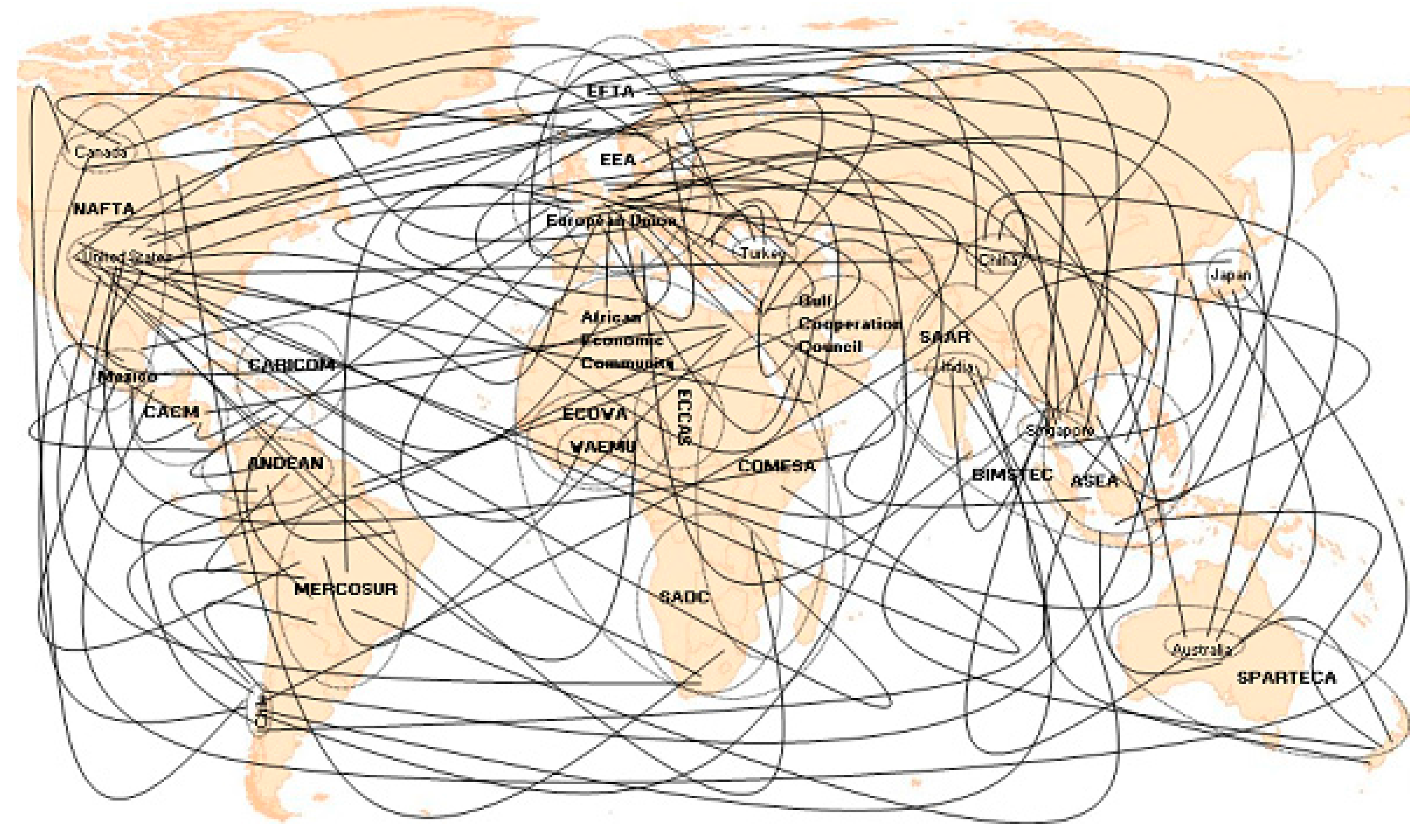
Bhagwati [17] drew an analogy between numerous trading relationship involving criss-crossing FTAs and tariff rates affected by multiple sources of origin and strands of spaghetti tangled in a bowl (see Figure 1) [23,24]. As is mentioned before, the Spaghetti Bowl Effect reduces the applicability of FTAs and increases the costs of participating firms, calling for due attention from both the academic and the practical sides.

While the Spaghetti Bowl Effect has been widely observed in many empirical studies, less is known about the exact mechanism of the Spaghetti Bowl Effect that affects a firm’s production and export decisions in the literature. As international trading has a close relationship with a global supply chain [26], we aim to fill this gap by providing analytical results of a firm’s production strategy under overlapping FTAs considering operational restrictions to meet different ROOs, in which upward or downward adjustment efforts of firms should be exerted to meet different environmental regulation conditions. In particular, we will show that adjusting a firm’s production capability to satisfy multiple ROOs can lead to the Spaghetti Bowl Effect, explicitly.

We consider a firm that currently exports its product to a country with an existing FTA and considers exporting to a new country under a different FTA. We show that a firm may strategically choose not to comply with the required ROO by the new FTA and pay the tariff instead, or choose to comply with a stricter ROO level than the level required by the new FTA. Such production decisions occur due to the costs associated with changing a firm’s production processes to meet different ROO requirements than required and different suppliers accordingly. We characterize these two unintended production decisions of the firm as two types of Spaghetti Bowl Effect. We also quantify the additional cost incurred from those two types of Spaghetti Bowl Effect.

To the best of our knowledge, the characterization and quantification of the Spaghetti Bowl Effect, in relation to a firm’s strategic production decisions, have not appeared in the literature as of yet, despite the considerable impact of ROO requirements on production costs and process adjustments of a firm, while stating that the minimum compliance to the rule is not the best strategy. We, thus, believe that our paper contributes to the literature by shedding light on this less explored issue of the Spaghetti Bowl Effect and its impact on a firm’s production decisions. We also believe that our paper contributes to the literature by extending our understanding the impact of multiple FTAs on firm’s global production and operations decisions.

The literature on global operations management that takes into account environmental issues related to an emission regulation (e.g., emission tax, emission cap-and-trade, etc.) is vast. Many operational factors have been discussed to investigate their impacts on the environment. We can take, as examples, compliance of regulation [27], supply chain design and procurement [28,29], product development [30], facility or retail store location [31,32], and choice and development of emission-reduction technology [33,34,35]. While these works mainly consider the impact of a specific regulations on each firm’s operational decisions, or compare multiple regulations on the same firm, we focus on the impact of multiple regulations imposed by overlapping FTAs on exporting firms. In particular, we investigate how a firm’s operational decisions change under multiple international regulations on environmental issues considering operational switching costs incurred by changing its production capability and suppliers to be in accordance with multiple ROOs. We, thus, believe that our paper contributes to the literature by extending our understanding of the impact of multiple FTAs on a firm’s global production and operations decisions.

The organization of this paper is as follows: in Section 2, we present our model; in Section 3, we provide the analysis of our model; we discuss policy implications in Section 4; and we conclude the paper in Section 5.

2. Model

We develop a model of a multinational firm which currently exports to one country (denoted by Country 1) under an FTA and considers exporting to a new country (denoted by Country 2) under a different FTA. The firm is assumed to act as a monopolist in Country 2. The inverse demand functions of the firm in Countries 1 and 2 are:

$${\mathrm{p}}_{\mathrm{k}}={\mathsf{\alpha }}_{\mathrm{k}}-{\mathrm{q}}_{\mathrm{k}}\mathrm{for}\mathrm{k}=1,2,$$

(1)

where ${\mathsf{\alpha }}_{\mathrm{k}}$ represents the potential market size and ${\mathrm{q}}_{\mathrm{k}}$ represents the exporting quantity to Country k (k = 1, 2). The inverse demand functions have been widely used in the literature; see, e.g., [3,36].

According to literature [37], ROOs are usually classified into types, such as (i) the value content rule (which should meet a minimum value ratio of corresponding local areas or regions); or (ii) the change in tariff classification (CTC) rule (which means the change in the Harmonized System (HS) Code of the raw material/components to the HS code of the final goods). Specifically, the ROO level in our paper represents the level of effort exerted to achieve a specific ROO requirement in an FTA.

We consider two categories of costs related to a firm’s production and export to the new country: the unit production cost and the conversion cost. First, we consider the unit production cost that increases with the required ROO levels. Let us denote the firm’s choice of compliance with the ROO level in country k by ${\mathrm{e}}_{\mathrm{k}}$, for k = 1, 2. Then, the unit production cost consists of the actual production cost, denoted by c, and the additional cost associated with the price of supplies used for production under the ROO level, denoted by ${\mathsf{\beta }\mathrm{e}}_{\mathrm{k}}$. Here, ${\mathsf{\beta }\mathrm{e}}_{\mathrm{k}}$ represents the additional unit production cost required to meet the ROO compliance level of ${\mathrm{e}}_{\mathrm{k}}$, because conforming to the given rule and utilizing the environmental components requires more effort and cost. Then, in Country 1, when the firm complies with an ROO level ${\mathrm{e}}_1$, the profit is given by:

$${\mathsf{\pi }}_1^{\mathrm{f}}\left({\mathrm{e}}_1,{\mathrm{q}}_1\right)={\mathrm{p}}_1{\mathrm{q}}_1-\left(\mathrm{c}+{\mathsf{\beta }\mathrm{e}}_1\right){\mathrm{q}}_1.$$

(2)

Second, we consider the cost of adjusting the firm’s current production capabilities to meet the new ROO level, which is referred to as the conversion cost. The conversion cost includes the costs associated with searching and managing qualified suppliers and changing product design and facilities under adjusting firms to new environmental standard or regulations. The conversion cost tends to increase as the difference in the two ROO levels under overlapping FTAs gets larger [38]. We consider this conversion cost to be the cost required to change the production process to comply with the new ROO requirement. Hence, this conversion cost is charged on the difference in ROO levels, independent of production quantities. This approach is observed in the literature [39]. We, thus, assume that the conversion cost increases, especially at an escalating rate, with the difference between two ROO levels in FTAs.

We model the conversion cost as follows. We represent the minimum ROO level required by the FTA in Country k as $\underset{\_}{{\mathrm{e}}_{\mathrm{k}}}$, which implies ${\mathrm{e}}_{\mathrm{k}}\ge \underset{\_}{{\mathrm{e}}_{\mathrm{k}}}$ under each FTA. If the firm currently complies with an ROO level $\underset{\_}{{\mathrm{e}}_1}$ in Country 1, and try to comply with an ROO level ${\mathrm{e}}_2$ in Country 2, the conversion cost is assumed to be in a convex relationship with the difference in the ROO levels between Country 1 and Country 2, represented by ${\mathrm{c}}_{\mathrm{con}}≔\mathsf{\gamma }{\left({\mathrm{e}}_2-\underset{\_}{{\mathrm{e}}_1}\right)}^2$. Here, $\mathsf{\gamma }$ denotes the cost coefficient to measure the efficiency in adjusting the firm’s production processes. Then, in Country 2, there should be two cost components incurred: the unit cost due to the given ROO level ${\mathrm{e}}_2$, and the cost incurred by changing the ROO level from $\underset{\_}{{\mathrm{e}}_1}$ in Country 1 to ${\mathrm{e}}_2$ in Country 2. The unit cost caused by the ROO level ${\mathrm{e}}_2$ is $\mathrm{c}+{\mathsf{\beta }\mathrm{e}}_2$, similarly to the situation in Country 1. The profit of the firm in Country 2 at the given ROO level ${\mathrm{e}}_2$, incorporating the conversion cost from $\underset{\_}{{\mathrm{e}}_1}$ to ${\mathrm{e}}_2$ is calculated as:

$${\mathsf{\pi }}_2^{\mathrm{f}}\left({\mathrm{e}}_2,{\mathrm{q}}_2\right)={\mathrm{p}}_2{\mathrm{q}}_2-\left(\mathrm{c}+{\mathsf{\beta }\mathrm{e}}_2\right){\mathrm{q}}_2-\mathsf{\gamma }{\left({\mathrm{e}}_2-\underset{\_}{{\mathrm{e}}_1}\right)}^2.$$

(3)

Then, the optimal exporting quantity of the firm under given compliance level ${\mathrm{e}}_1$ in Country 1 is:

$${\mathrm{q}}_1^{\mathrm{f}}\left({\mathrm{e}}_1\right):=\arg \underset{{\mathrm{q}}_1}{\max }{\mathsf{\pi }}_1^{\mathrm{f}}\left({\mathrm{e}}_1,{\mathrm{q}}_1\right)=\frac{{\mathsf{\alpha }}_1-\mathrm{c}-{\mathsf{\beta }\mathrm{e}}_1}{2},$$

(4)

and the corresponding profit is obtained by:

$${\Pi }_1^{\mathrm{f}}\left({\mathrm{e}}_1\right)≔{\mathsf{\pi }}_1^{\mathrm{f}}\left({\mathrm{e}}_1,{\mathrm{q}}_1^{\mathrm{f}}\left({\mathrm{e}}_1\right)\right)=\frac{{({\mathsf{\alpha }}_1-\left(\mathrm{c}+{\mathsf{\beta }\mathrm{e}}_1\right))}^2}{4}.$$

(5)

It is easy to show that Equation (5) is decreasing in ${\mathrm{e}}_1$ when Equation (4) is nonnegative. Since the firm is assumed to already comply with the ROO already Country 1, the firm’s optimal choice of compliance level is $\underset{\_}{{\mathrm{e}}_1}$ to minimize its unit production cost, which yields ${\Pi }_1^{\mathrm{f}}\left(\underset{\_}{{\mathrm{e}}_1}\right).$

Now we consider the firm’s decision in Country 2. The firm has two choices in Country 2. The firm can enjoy zero tariff by complying with the ROO of the FTA in Country 2, or, alternatively, may ignore the benefit of the FTA and pay the traditional tariff instead.

Firstly, we consider the decision of the firm when complying with the ROO of the FTA. The firm’s optimal production quantity for Country 2 under the given compliance level ${\mathrm{e}}_2$ is easily obtained by:

$${\mathrm{q}}_2^{\mathrm{f}}\left({\mathrm{e}}_2\right):=\arg \underset{{\mathrm{q}}_2}{\max }{\mathsf{\pi }}_2^{\mathrm{f}}\left({\mathrm{e}}_2,{\mathrm{q}}_2\right)=\frac{{\mathsf{\alpha }}_2-\mathrm{c}-{\mathsf{\beta }\mathrm{e}}_2}{2}.$$

(6)

Applying the quantity obtained, the firm’s profit in country 2 becomes:

$$\begin{gathered} {\Pi }_2^{\mathrm{f}}\left({\mathrm{e}}_2\right)≔{\mathsf{\pi }}_2^{\mathrm{f}}\left({\mathrm{e}}_2,{\mathrm{q}}_2^{\mathrm{f}}\left({\mathrm{e}}_2\right)\right) \\ =\frac{1}{4}({\left({\mathsf{\alpha }}_2-\mathrm{c}\right)}^2-4\mathsf{\gamma }{\underset{\_}{{\mathrm{e}}_1}}^2-{\mathrm{e}}_2\left(2\mathsf{\beta }\left({\mathsf{\alpha }}_2-\mathrm{c}\right)-8\mathsf{\gamma }\underset{\_}{{\mathrm{e}}_1}+\left(4\mathsf{\gamma }-{\mathsf{\beta }}^2\right){\mathrm{e}}_2\right)). \end{gathered}$$

(7)

In this situation, the firm’s choice of the ROO level ${\mathrm{e}}_2$ in Country 2 might not be $\underset{\_}{{\mathrm{e}}_2}$ due to the conversion cost, although $\underset{\_}{{\mathrm{e}}_2}$ provides the lowest unit production cost. The compliance level for Country 2 that maximizes (7), denoted by ${\mathrm{e}}_2^{*}$ is then obtained as:

$${\mathrm{e}}_2^{*}=\frac{\mathsf{\beta }\mathrm{c}+4\mathsf{\gamma }\underset{\_}{{\mathrm{e}}_1}-{\mathsf{\beta }\mathsf{\alpha }}_2}{4\mathsf{\gamma }-{\mathsf{\beta }}^2},$$

(8)

with the corresponding profit of ${\Pi }_2^{\mathrm{f}}\left({\mathrm{e}}_2^{*}\right)$.

Secondly, we consider the decision of the firm when the firm chooses to pay the traditional tariff instead of complying with the ROO of the FTA. Although eco-friendly contents preference is related with ROO (especially the case of exporting to high-regulating countries), complying with the environmental standards of Country 2 is required for both tariff and ROO selections [40]. We denote the tariff rate of Country 2 by ${\mathrm{t}}_2$. Without the FTA in Country 2, the firm that wishes to export to Country 2 should pay the tariff rate ${\mathrm{t}}_2$, which makes the unit cost $\mathrm{c}+{\mathrm{t}}_2$. Then the profit of the firm in Country 2 in this situation is given by:

$${\mathsf{\pi }}_2^{\mathrm{t}}\left({\mathrm{t}}_2,{\mathrm{q}}_2\right)={\mathrm{p}}_2{\mathrm{q}}_2-\left(\mathrm{c}+{\mathrm{t}}_2\right){\mathrm{q}}_2.$$

(9)

To avoid trivial results we assume $\mathrm{c}+{\mathsf{\beta }\mathrm{e}}_2<\mathrm{c}+{\mathrm{t}}_2$, since otherwise the tariff should be always chosen over the FTA. The optimal production quantity for Country 2 in this situation is:

$${\mathrm{q}}_2^{\mathrm{t}}\left({\mathrm{t}}_2\right):=\arg \underset{{\mathrm{q}}_2}{\max }{\mathsf{\pi }}_2^{\mathrm{t}}\left({\mathrm{t}}_2,{\mathrm{q}}_2\right)=\frac{{\mathsf{\alpha }}_2-\mathrm{c}-{\mathrm{t}}_2}{2}.$$

(10)

Applying this quantity, the profit of the firm in Country 2 when paying the tariff becomes:

$${\Pi }_2^{\mathrm{t}}\left({\mathrm{t}}_2\right)={\mathsf{\pi }}_2^{\mathrm{t}}\left({\mathrm{t}}_2,{\mathrm{q}}_2^{\mathrm{t}}\left({\mathrm{t}}_2\right)\right)=\frac{{\left({\mathsf{\alpha }}_2-\mathrm{c}-{\mathrm{t}}_2\right)}^2}{4}.$$

(11)

In the next section, we analyze the firm’s optimal choice in Country 2 based on the above models.

3. Analysis

In this section, we define and quantify the Spaghetti Bowl Effect by analyzing the firm’s decision in Country 2. The firm’s choice should be either to comply with the ROO required in the FTA of Country 2, or to pay the traditional tariff. When choosing to pay the traditional tariff, the corresponding profit of the firm is ${\Pi }_2^{\mathrm{t}}\left({\mathrm{t}}_2\right)$, as calculated in Equation (11).

On the other hand, when the firm chooses to comply with the ROO to get the tariff exemption provided by the FTA, it should compare ${\mathrm{e}}_2^{*}$ with $\underset{\_}{{\mathrm{e}}_2}$. If ${\mathrm{e}}_2^{*}\ge \underset{\_}{{\mathrm{e}}_2}$, the firm should choose the ROO level of ${\mathrm{e}}_2^{*}$, since it gives the lowest production cost as well as meets the required ROO level. However, if ${\mathrm{e}}_2^{*}<\underset{\_}{{\mathrm{e}}_2}$, ${\mathrm{e}}_2^{*}$ is no longer a feasible ROO level since it falls below the minimum required level; hence, the firm should be only able to consider $\underset{\_}{{\mathrm{e}}_2}$ for the FTA. Based on this consideration, we can classify the strategic decisions of the firm into the following three cases.

$$\mathrm{Case}1:{\mathrm{e}}_2^{*}\le \underset{\_}{{\mathrm{e}}_2}\mathrm{and}{\Pi }_2^{\mathrm{f}}\left(\underset{\_}{{\mathrm{e}}_2}\right)\ge {\Pi }_2^{\mathrm{t}}\left({\mathrm{t}}_2\right).$$

In this case, the minimum required ROO level $\left(\underset{\_}{{\mathrm{e}}_2}\right)$ to a firm is higher than the firm’s profit-maximizing ROO level $\left({\mathrm{e}}_2^{*}\right)$. The firm chooses to meet the minimum required ROO level to exploit the FTA conditions when it is more beneficial than paying the tariff. In this situation, the FTA works normally as intended.

$$\mathrm{Case}2:{\Pi }_2^{\mathrm{t}}\left({\mathrm{t}}_2\right)>{\Pi }_2^{\mathrm{f}}\left(\max \left\{\underset{\_}{{\mathrm{e}}_2},{\mathrm{e}}_2^{*}\right\}\right).$$

In Case 2, the firm strategically ignores the ROO requirements and chooses to pay the traditional tariff instead. Thus, the intended benefit of the FTA is not realized and the gap of profits achieved by the tariff in Country 2 (${\mathrm{t}}_2)$ and the minimum required ROO level $\left(\underset{\_}{{\mathrm{e}}_2}\right)$ explains one type of the Spaghetti Bowl Effect. This occurs when the conversion cost to change the firm’s process to reach the required ROO level in Country 2 is so high that it is outperformed by the profit gained by paying the tariff.

$$\mathrm{Case}3:{\mathrm{e}}_2^{*}>\underset{\_}{{\mathrm{e}}_2}{\mathrm{and}\Pi }_2^{\mathrm{f}}\left({\mathrm{e}}_2^{*}\right)\ge {\Pi }_2^{\mathrm{t}}\left({\mathrm{t}}_2\right).$$

In Case 3, the firm can further increase its profit by setting the compliance level higher than the minimum required ROO. As a result, the firm’s choice of ROO compliance level is different from the minimum required ROO level in the FTA. This situation occurs when Country 2’s required ROO level is lower than that of Country 1, and the conversion cost prohibits the firm from reaching Country 2’s ROO level. The gap of profits achieved by the profit-maximizing compliance level $\left({\mathrm{e}}_2^{*}\right)$ and the minimum ROO level $\left(\underset{\_}{{\mathrm{e}}_2}\right)$ quantifies another type of the Spaghetti Bowl Effect.

As shown in Case 1, the firm involved with overlapping multiple FTAs, most desirably may choose the ROO level as intended under each FTA. However, we observe that it is not always the case as shown in Case 2 and Case 3. The firm may strategically choose to pay the tariff instead of utilizing the FTA in country 2 (Case 2), or choose an ROO level that is stricter than the minimum required ROO level in the FTA for Country 2 (Case 3). These latter two cases characterize two different types of firm’s decisions under overlapping FTAs that deviate from complying with the minimum required ROOs as intended in these FTAs, i.e., the Spaghetti Bowl Effect.

In the following propositions, we identify the conditions when each type of the Spaghetti Bowl Effect occurs in terms of the trading environment (minimum required ROO level, tariff rate, and market size) and the production environment (production cost and conversion efficiency) of the firm. Proposition 1 represents the case where the FTA in Country 2 is not effective, which we refer to as Type I of the Spaghetti Bowl Effect. This corresponds to the situation described in Case 2. All proofs are located in Appendix A.

Proposition 1 (Type I of the Spaghetti Bowl Effect).

The firm chooses to pay the tariff in Country 2 if the tariff level $t_2$ and the minimum required ROOs for Country 1 and Country 2 satisfy either of the following conditions:

(i) 

$\underset{\_}{e_2}<e_2^{*}and\underset{\_}{e_1}\in \left({\psi }_{1a},{\psi }_{1b}\right),$ where

$${\psi }_{1a}=\frac{\left({\alpha }_2-c-t_2\right)\left(1-\sqrt{\frac{4\gamma -{\beta }^2}{4\gamma }}\right)+t_2}{\beta }and{\psi }_{1b}=\frac{\left({\alpha }_2-c-t_2\right)\left(1+\sqrt{\frac{4\gamma -{\beta }^2}{4\gamma }}\right)+t_2}{\beta }$$

(12)

(ii) 

$\underset{\_}{e_2}\ge e_2^{*}$ and $\underset{\_}{e_2}\notin \left[{\psi }_{2a},{\psi }_{2b}\right]$, where

• ${\psi }_{2a}=\frac{-\beta \left({\alpha }_2-c\right)+4\gamma \underset{\_}{e_1}-\sqrt{{\left(\beta \left({\alpha }_2-c\right)-4\gamma \underset{\_}{e_1}\right)}^2+\left(4\gamma -{\beta }^2\right)\left(t_2\left(2{\alpha }_2-2c-t_2\right)-4\gamma {\underset{\_}{e_1}}^2\right)}}{4\gamma -{\beta }^2}$ and
• ${\psi }_{2b}=\frac{-\beta \left({\alpha }_2-c\right)+4\gamma \underset{\_}{e_1}+\sqrt{{\left(\beta \left({\alpha }_2-c\right)-4\gamma \underset{\_}{e_1}\right)}^2+\left(4\gamma -{\beta }^2\right)\left(t_2\left(2{\alpha }_2-2c-t_2\right)-4\gamma {\underset{\_}{e_1}}^2\right)}}{4\gamma -{\beta }^2}$.

Then, Type I of the Spaghetti Bowl Effect is quantified by ${\Pi }_2^t\left(t_2\right)-{\Pi }_2^f\left(\underset{\_}{e_2}\right)$.

Proposition 2 represents the other situation where the firm chooses an ROO compliance level that is different from the minimum required ROO level in Country 2, which we refer to as Type II of the Spaghetti Bowl Effect. This corresponds to the situation described in Case 3.

Proposition 2 (Type II of the Spaghetti Bowl Effect).

The firm chooses the profit-maximizing ROO compliance level $e_2^{*}$ that is higher than the minimum ROO compliance level in Country 2 when the tariff level $t_2$ and the minimum required ROOs for Country 1 and Country 2 satisfies the following condition:

$e_2^{*}>\underset{\_}{e_2}$ and $\underset{\_}{e_1}\notin \left({\psi }_{1a},{\psi }_{1b}\right)$ where ${\psi }_{1a}and{\psi }_{1b}$ defined in (12).

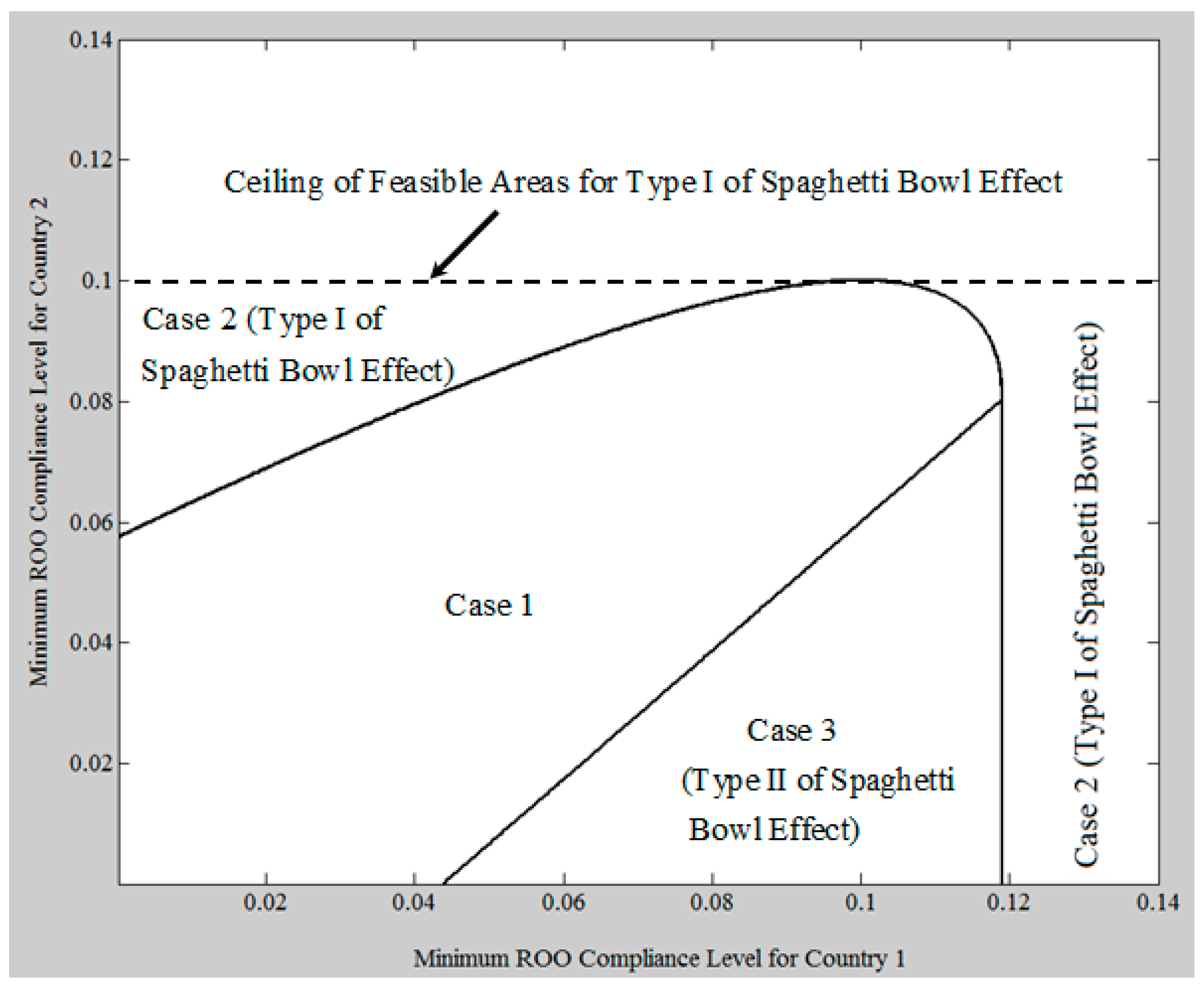
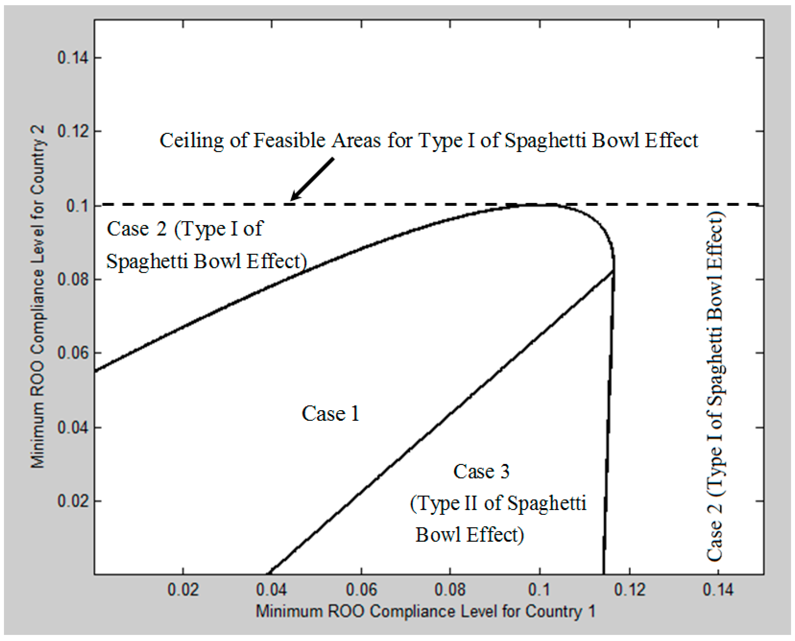
Figure 2 illustrates the firm’s decision in Country 2 for the three cases defined above. Note that Type I of the Spaghetti Bowl Effect occurs in Case 2 and Type II of the Spaghetti Bowl Effect occurs in Case 3. We observe from the figure that Type I of the Spaghetti Bowl Effect occurs when the minimum compliance levels of the two countries’ FTAs are highly deviated. In such situations, the conversion costs dominate the efficiency of FTAs, resulting in choosing the traditional tariff scheme. On the other hand, if the minimum required ROO level in Country 2 is significantly lower than that of Country 1, the conversion cost discourages the firm from choosing the minimum ROO level for Country 2, incurring Type II of the Spaghetti Bowl Effect. When the two minimum required ROOs in the two countries are not significantly different from each other, we observe that the intended outcome of FTAs, i.e., Case 1, is achieved. In Figure 2, we observe a ceiling of the feasible area for Type I of the Spaghetti Bowl Effect for Country 2. The ceiling is formed by the condition $\mathrm{c}+{\mathsf{\beta }\mathrm{e}}_2=\mathrm{c}+{\mathrm{t}}_2$, which is located below Equation (9). This condition is imposed to identify and exclude the trivial case in our analysis. When the minimum ROO compliance level for Country 2 falls above the ceiling, the tariff rate falls below the unit cost associated with achieving an ROO level with ${\mathsf{\beta }\mathrm{e}}_2$. In this situation, it is always more profitable for the firm to pay the tariff in Country 2 instead of complying with the minimum required ROO level in the FTA.

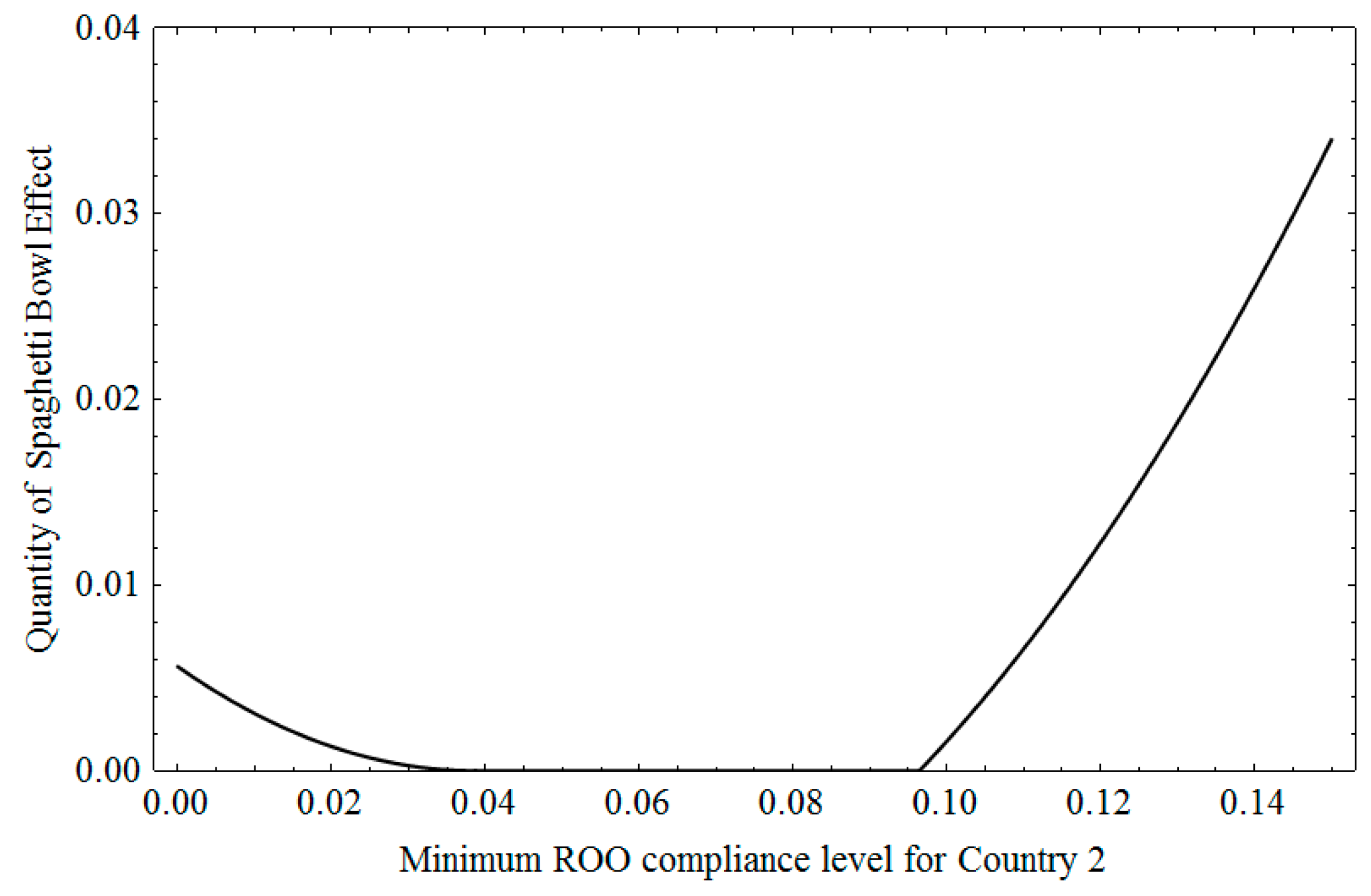
Recall that the amount of the Spaghetti Bowl effect is quantified by calculating the difference between the profit under complying with the minimum required ROO level and the profit under tariff or a higher ROO level than the minimum required one in Propositions 1 and 2. Figure 3 shows the quantity of the Spaghetti Bowl Effect in each type under a given $\underset{\_}{{\mathrm{e}}_1}$. We observe from the figure that the quantity of the Spaghetti Bowl Effect tends to increase when the difference between the ROO levels in the FTAs of Country 1 and Country 2 increases. This result also suggests that an effort to reduce the gap between the ROO levels in different FTAs would make the FTAs more effective and reduce the likelihood of an unintended Spaghetti Bowl Effect.

The next proposition shows that the Spaghetti Bowl Effect must occur as long as the conversion coefficient exceeds a certain level.

Proposition 3.

Unless $\underset{\_}{e_1}=\underset{\_}{e_2}$ the Spaghetti Bowl Effect always occurs when $\gamma$ exceeds

$$\chi =max\left\{\frac{{\beta }^2{\left({\alpha }_2-c-t_2\right)}^2}{4\left(\beta \underset{\_}{e_1}-t_2\right)\left(2{\alpha }_2-2c-t_2-\beta \underset{\_}{e_1}\right)},\frac{(t_2-\beta \underset{\_}{e_2})\left(2{\alpha }_2-2c-t_2-\beta \underset{\_}{e_2}\right)}{4{\left(\underset{\_}{e_1}-\underset{\_}{e_2}\right)}^2},\frac{\beta \left({\alpha }_2-c-\beta \underset{\_}{e_2}\right)}{4\left(\underset{\_}{e_1}-\underset{\_}{e_2}\right)}\right\}.$$

Proposition 3 shows that Spaghetti Bowl Effect always occurs if the firm’s conversion coefficient is sufficiently high such that it is too costly to change the firm’s production capability to meet a different ROO from the current level. The conversion cost tends to be high when the production system is highly sensitive to changes of suppliers. For example, the ROOs in the textile and apparel industry are more restrictive than other sectors [7] and, thus, the conversion costs are high, since the materials supplied to the industry are subject to tighter environmental regulations. For similar reasons, the agriculture industry also has a high conversion cost.

In the next proposition, we investigate the impact of conversion efficiency on the quantity of the Spaghetti Bowl Effect. Proposition 4 shows that the loss of firm’s profit due to the Spaghetti Bowl Effect amplifies with the decrease of the conversion efficiency.

Proposition 4.

• The amount for Type I of the Spaghetti Bowl Effect increases as the conversion efficiency of a firm decreases (i.e., as $\gamma$ increases) when $\underset{\_}{e_1}\ne \underset{\_}{e_2}$.
• The amount for Type II of the Spaghetti Bowl Effect increases as the conversion efficiency of a firm decreases (i.e., as $\gamma$ increases).

Since the conversion coefficient plays a significant role in the quantity of the Spaghetti Bowl Effect, Propositions 3 and 4 imply that the regulators of FTAs should consider firms’ overall conversion efficiency in determining the minimum required ROOs. In addition, it is recommended that the regulators seek for policies to help the firms invest in the conversion efficiency of production capabilities to reduce the likelihood of unintended outcomes under multiple overlapping FTAs.

The above analysis can be extended to more general cases with competing firms. In Appendix B, we added an investigation of the duopoly case, and find that our insights obtained under a monopoly market continue to hold under a duopoly market.

4. Policy Implications

In this section, we discuss how policy makers in one country may avoid the Spaghetti Bowl Effect when establishing FTAs with multiple countries.

We first consider an ROO level in an FTA. Our result obtained from Propositions 1 and 2 suggest that any type of the Spaghetti Bowl Effect may occur when the ROO levels of multiple FTAs are significantly different. This suggestion is in line with empirical research such as [20]. If an existing FTA and the newly-established FTA would have significantly different ROO levels, the tariff exemption from one country to the other is not effective as intended. Some firms choose to pay the tariff without taking advantage of tariff exemption from FTA and the others may choose to maintain an even stricter ROO level than that is required in the FTA. Either a firm pays the tariff or produces a product under a stricter ROO level than that is imposed in an FTA, one country is placed in a relatively inferior position in terms of benefits from an FTA than the other counterparty country.

Since ROO levels are involved with suppliers in one country and their materials, it is important to consider the impact of changing suppliers and their materials procured for multinational firm’s production of their products accordingly. This suggests the need for understanding a firm’s operational conditions carefully when negotiating an FTA. Such operational conditions include the types of materials supplied to a firm’s production process and their qualification to an ROO condition. Additionally, if some suppliers should be replaced with others by some ROO conditions, the impact of this change on a firm’s production process, i.e., how much of its process is affected by the change of suppliers and what are the associated costs in adjusting the production facilities, if any, to accommodate the new suppliers. Information on these operational conditions should be collected from individual firms who are intended to enter the market of the target country with the new FTA. Thus, operational conditions and production decisions should be properly considered when negotiating the required ROO levels in an FTA.

Propositions 3 and 4 suggest the need for an understanding of a firm’s conversion coefficient in its production. They show that when the conversion coefficient reaches a threshold, the Spaghetti Bowl Effect is more likely to occur for any ROO levels in multiple FTAs. This calls for policies to reduce firm’s conversion coefficient. Reduction of firm’s conversion coefficient can be achieved by developing R and D on technologies for a flexible production process. This includes developing new facilities or changing the sequence of production processes to make changes of suppliers easily accommodated. For example, a firm may adopt a production facility that can process various types of materials in its production system instead of maintaining a facility that is limited to a specific material [41]. In addition, a firm may change its production process such that a material-specific process is placed later in its process such that impact of materials changes is minimized. This is related to so-called delayed differentiating in operational strategy [42]. A policy that promotes these flexible production processes should be grounded on a careful understanding of firms’ production process. We, thus, emphasize the importance of operational considerations for policy- and decision-makers in establishing FTAs.

Note that we have analyzed the firm’s decisions when it operates in two countries. As more countries and FTAs are involved in a firm’s production decisions, the degree of required changes to meet different ROOs would not be the same. For example, one supplier may be qualified for more than two different ROOs at the same time. On the other hand, each ROO of an FTA may require a different supplier to be used in a firm’s production. Thus, in the case of multiple countries’ FTAs, it is important to identify how much of a firm’s production, capability, and supplier may be qualified for multiple ROOs and how much of them should change for each ROO and FTA. These would require a more complicated analysis, but we still believe that a firm’s production strategy falls into the three cases we have considered in our analysis.

5. Conclusions

This paper studies a multinational firm’s operational decision in the presence of multiple ROOs in FTAs. Especially, we investigate the unintended outcome of overlapping FTAs: an effect called the Spaghetti Bowl Effect. We developed a simple model of a multinational firm which currently exports to Country 1 under an FTA and considers exporting to Country 2 with a different FTA. We considered two different types of costs: the unit cost for production and the conversion cost of production capability to meet different ROO levels. Then we investigated the firm’s strategic production decision for Country 2. The firm may either pay the traditional tariff in Country 2 or take the advantage of tariff exemptions from complying with the required ROO level for the FTA in Country 2.

Our analysis shows that different ROO requirement levels across overlapping FTAs can cause a firm to choose not to comply with the ROO conditions and pay the tariff instead or it can cause the firm to choose a compliance level that is different from the minimum required ROO level under the FTA. These two situations are characterized by Type I and Type II of the Spaghetti Bowl Effect, respectively. We identify the conditions where these types of the Spaghetti Bowl Effect occur. Interestingly, we show that if the conversion efficiency is low enough, any type of the Spaghetti Bowl Effect should occur.

We extended previous Spaghetti Bowl Effect research by highlighting the new type which stemmed from the ROO disparity between two FTAs. The previous research focused on the effects of ROO in one country [1,2], however, we attempted to compare two ROOs, which have been applied to different countries.

The result suggests that the regulators should consider adopting measures to make ROO requirements across different FTAs more consistent. Our suggestion here is in line with the work of [7,20], which argued that dilution of rules of origin (ROOs) is required to minimize the Spaghetti Bowl Effect.

In addition, since the conversion efficiency affects the quantity of the Spaghetti Bowl Effect significantly, regulators should consider policies to motivate the firms to improving the conversion efficiency of their production systems. Our result also provides implications to the managers for the investment in the flexibility of the production capability to incorporate different ROO levels more efficiently across multiple countries.

Several future directions remain worthy of studying. First, we used a simplified inverse demand function where the price sensitivity is one. While we believe that our structural properties hold with a more general demand function, it would be interesting to investigate the impact of price sensitivity in future studies. Second, as discussed in Section 4, it would be important to investigate how a firm’s production strategy would change when more than three ROOs are involved. Lastly, the limitations of our work such as the linear demand function and standard rate based tariff scheme should be indicated. More realistic models can be developed by extending our work by incorporating more practical settings, such as a CES demand function and the ad-valorem tariff schemes.