
Characteristics of Suspended Sediment Loadings under Asian Summer Monsoon Climate Using the Hydrological Simulation Program-FORTRAN

Abstract
:1. Introduction
2. Materials and Methods
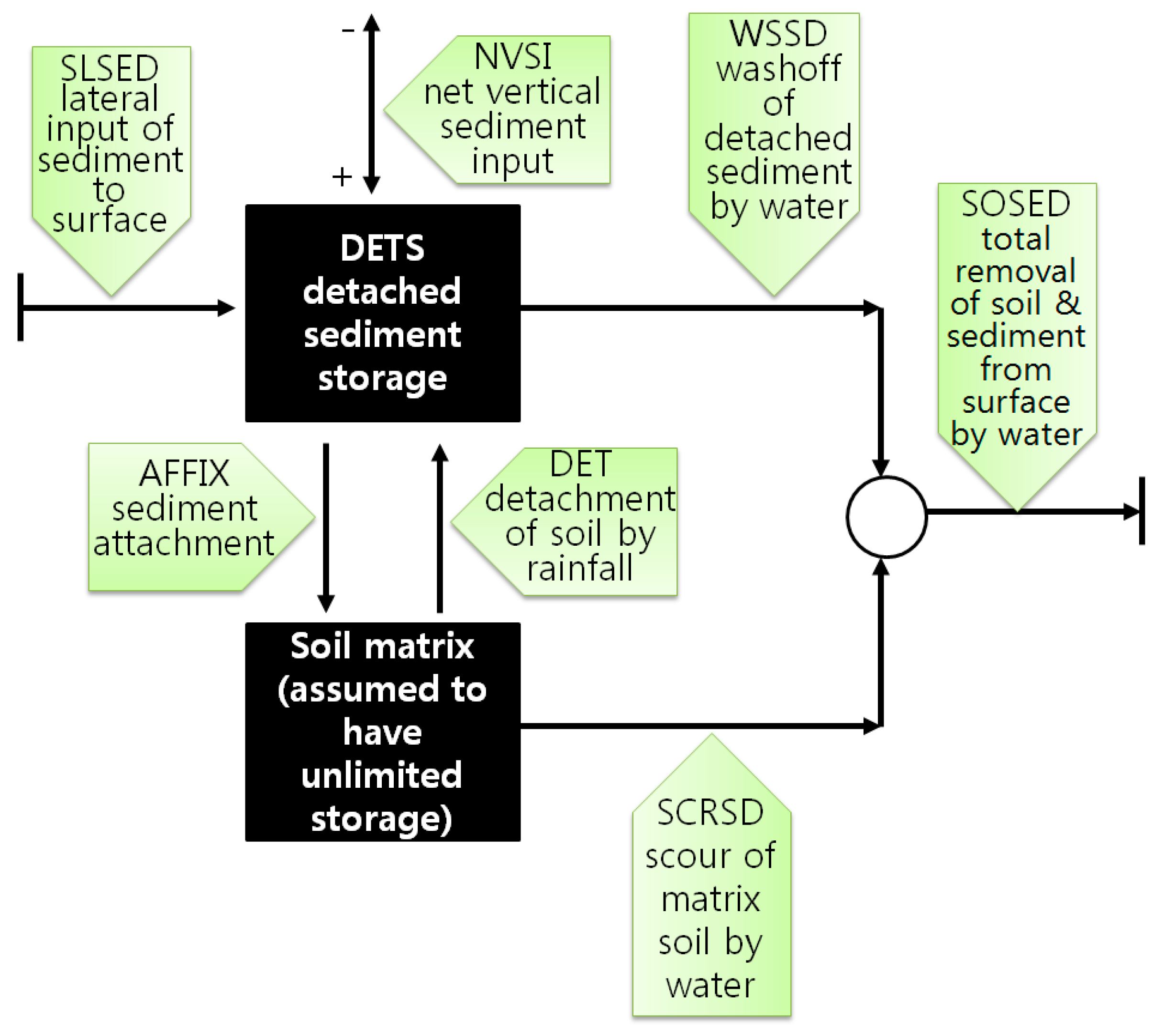
2.1. Overview of Hydrologic Simulation Program-FORTRAN (HSPF)
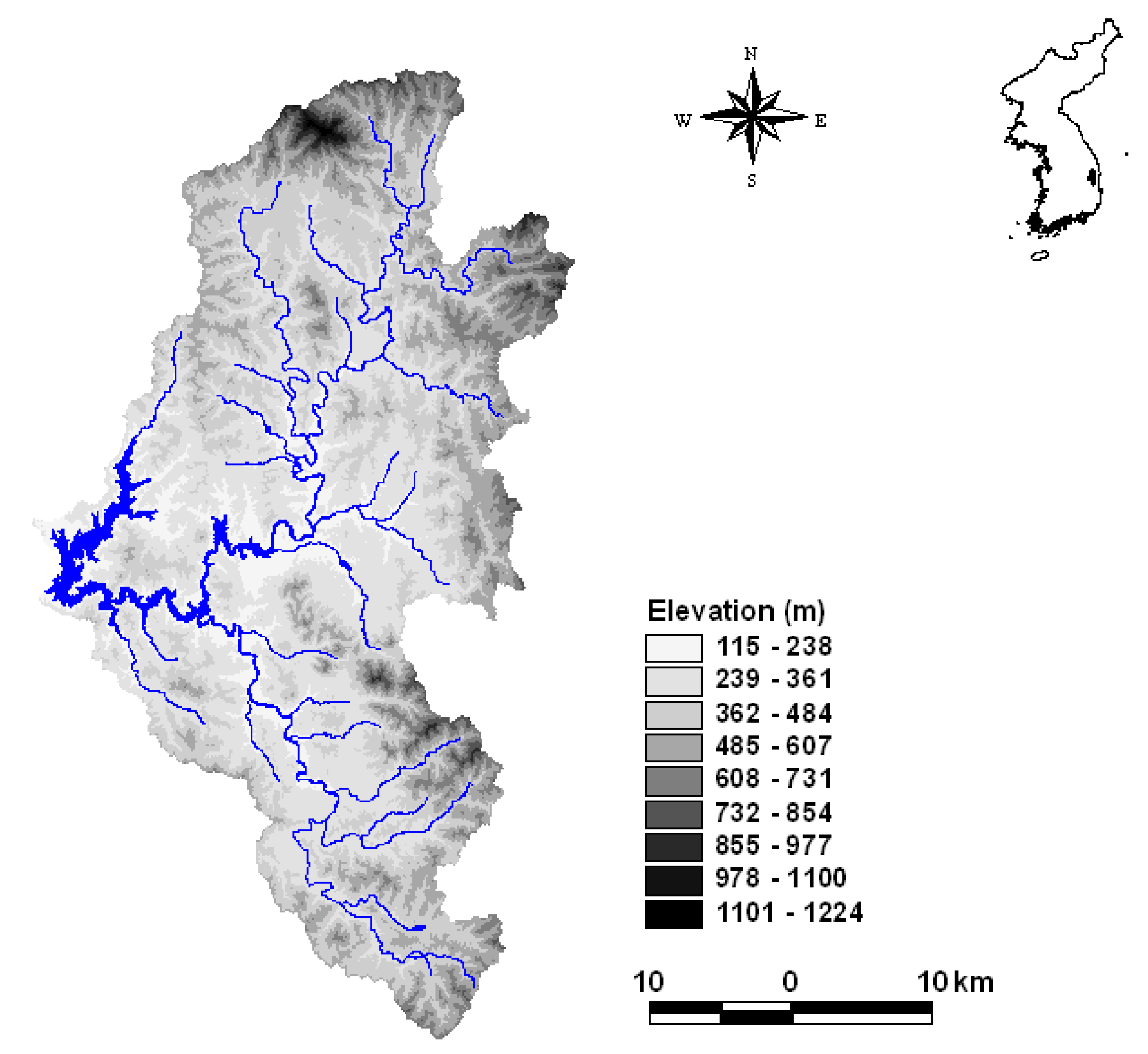
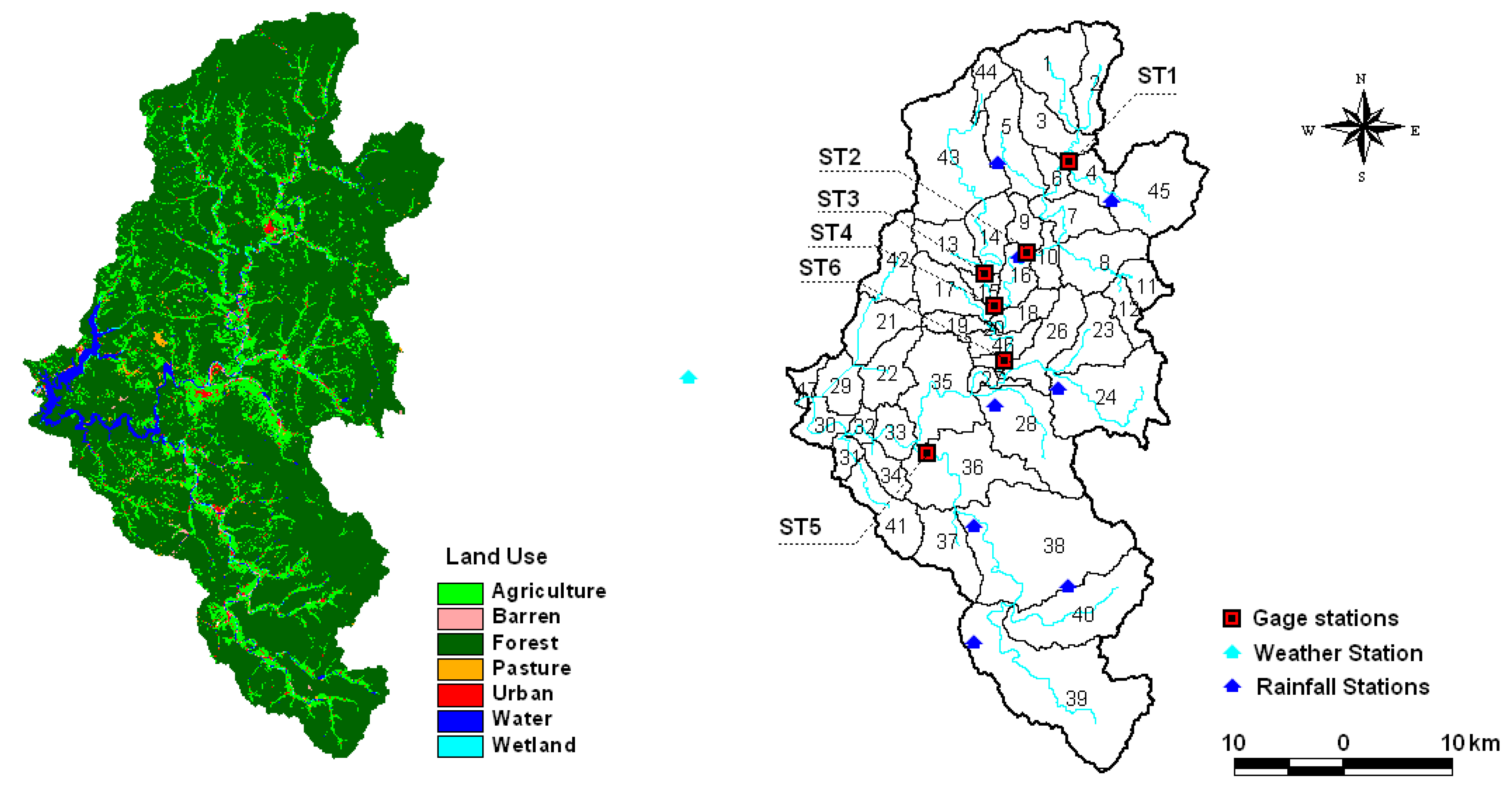
2.2. Study Area
2.3. Data Preparation
2.4. HSPF Calibration
3. Results and Discussion
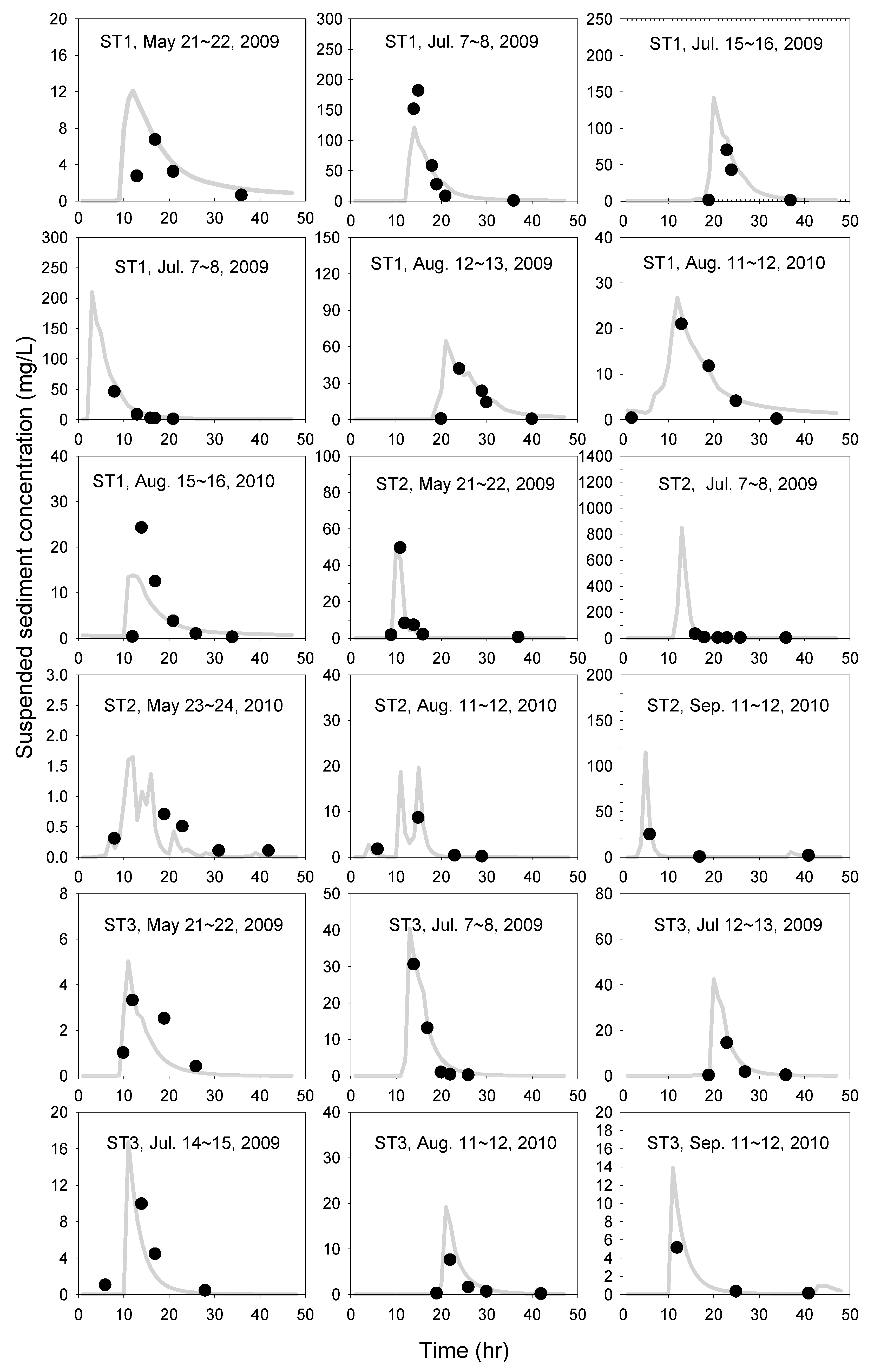
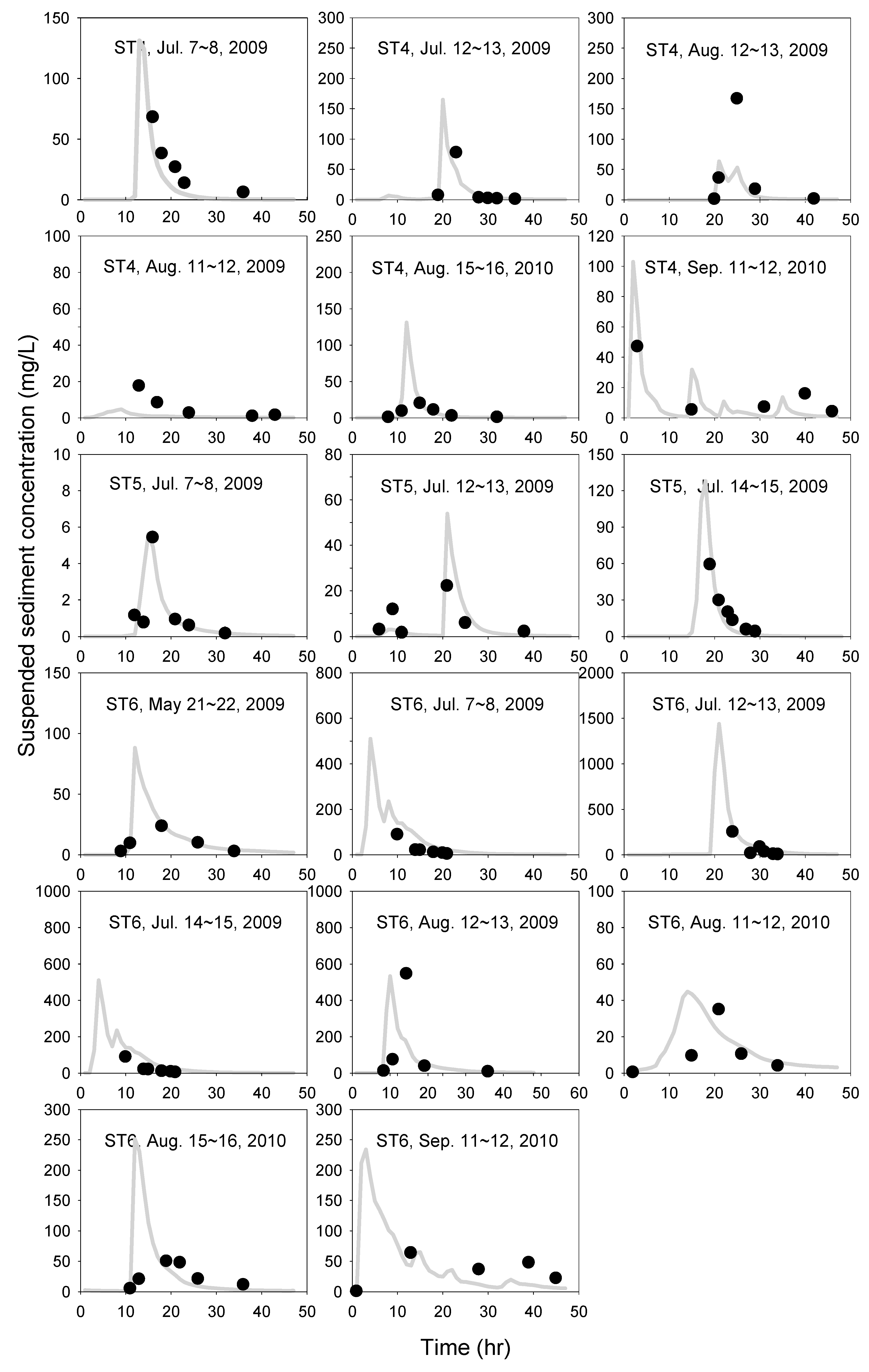
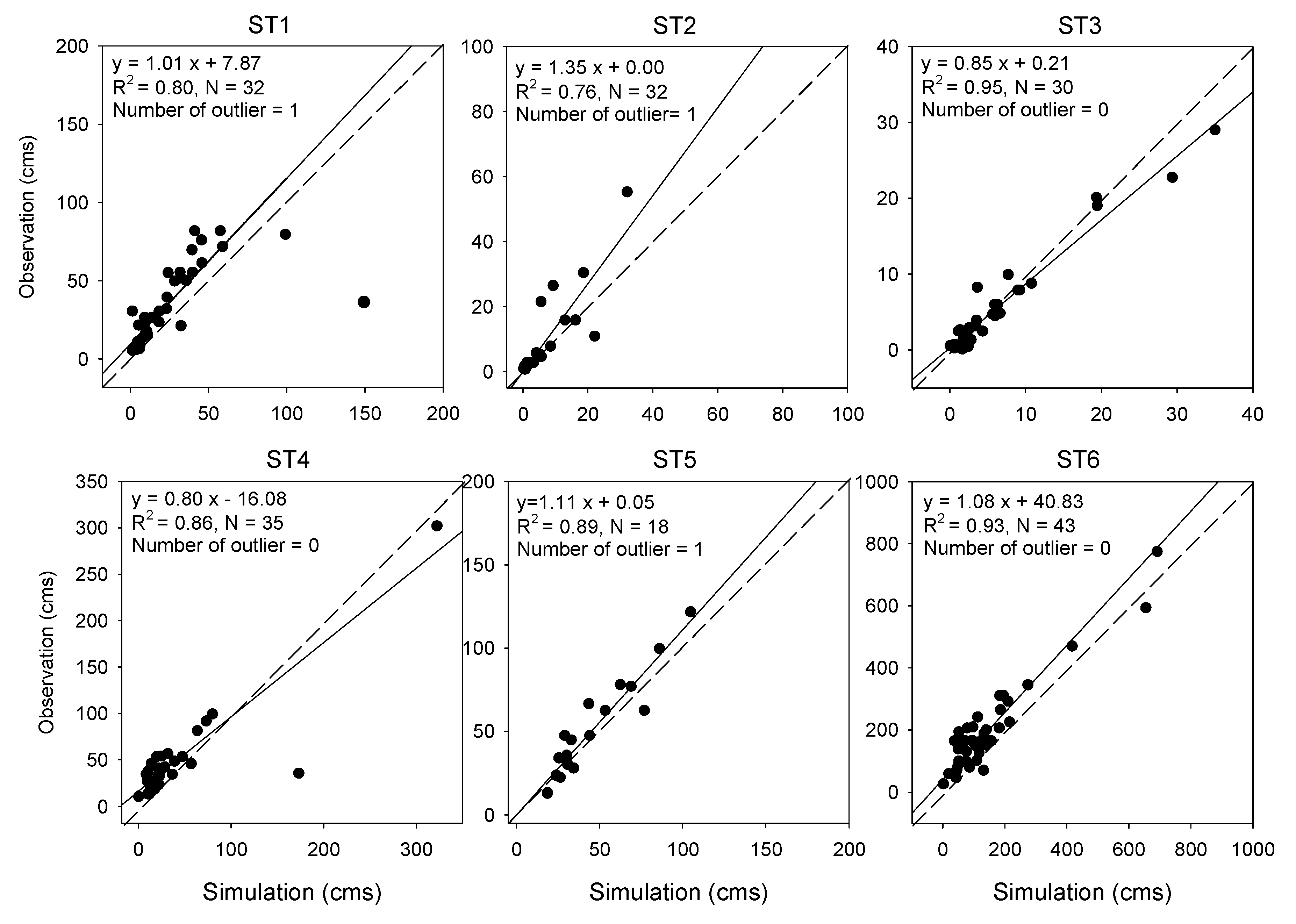
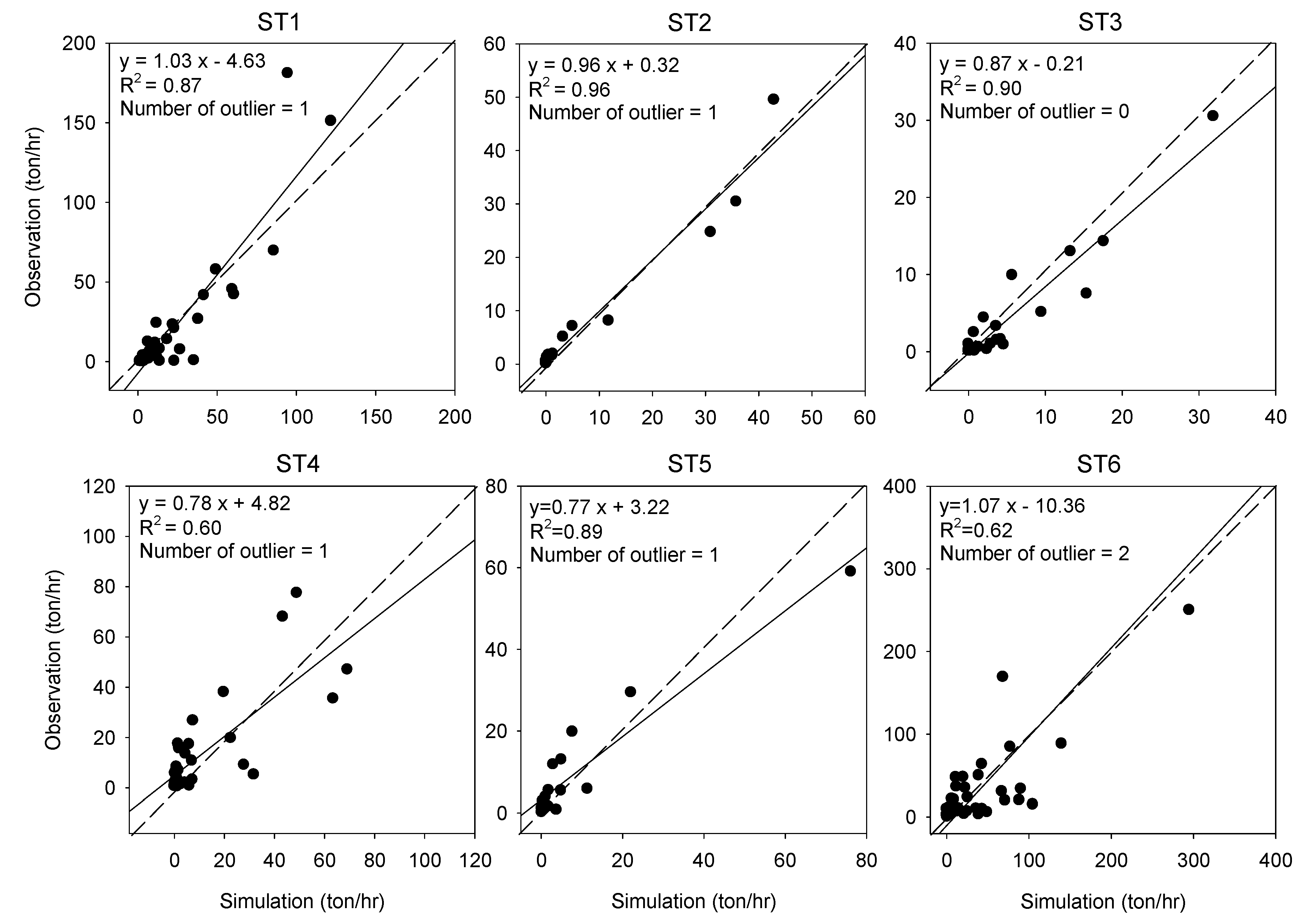
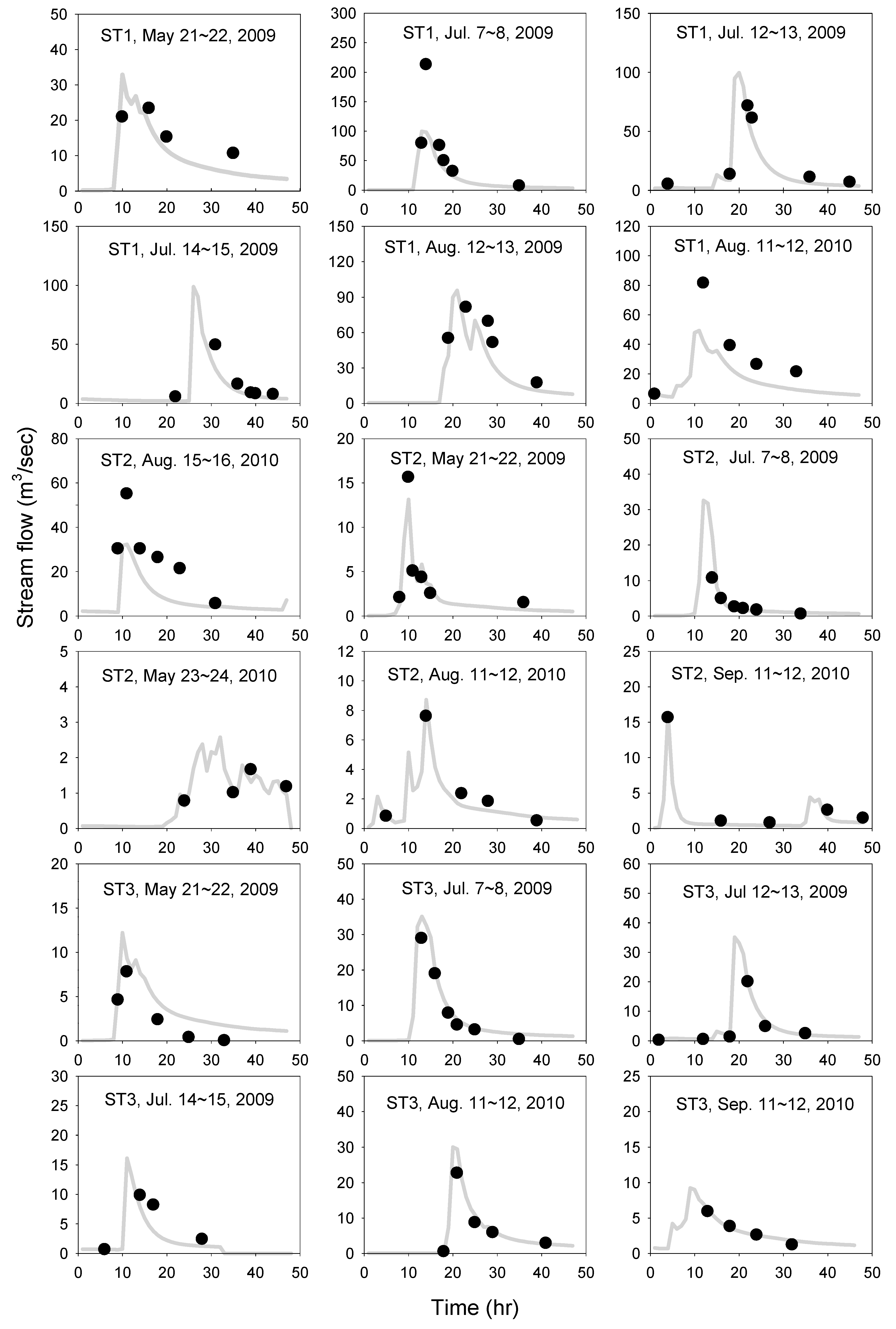
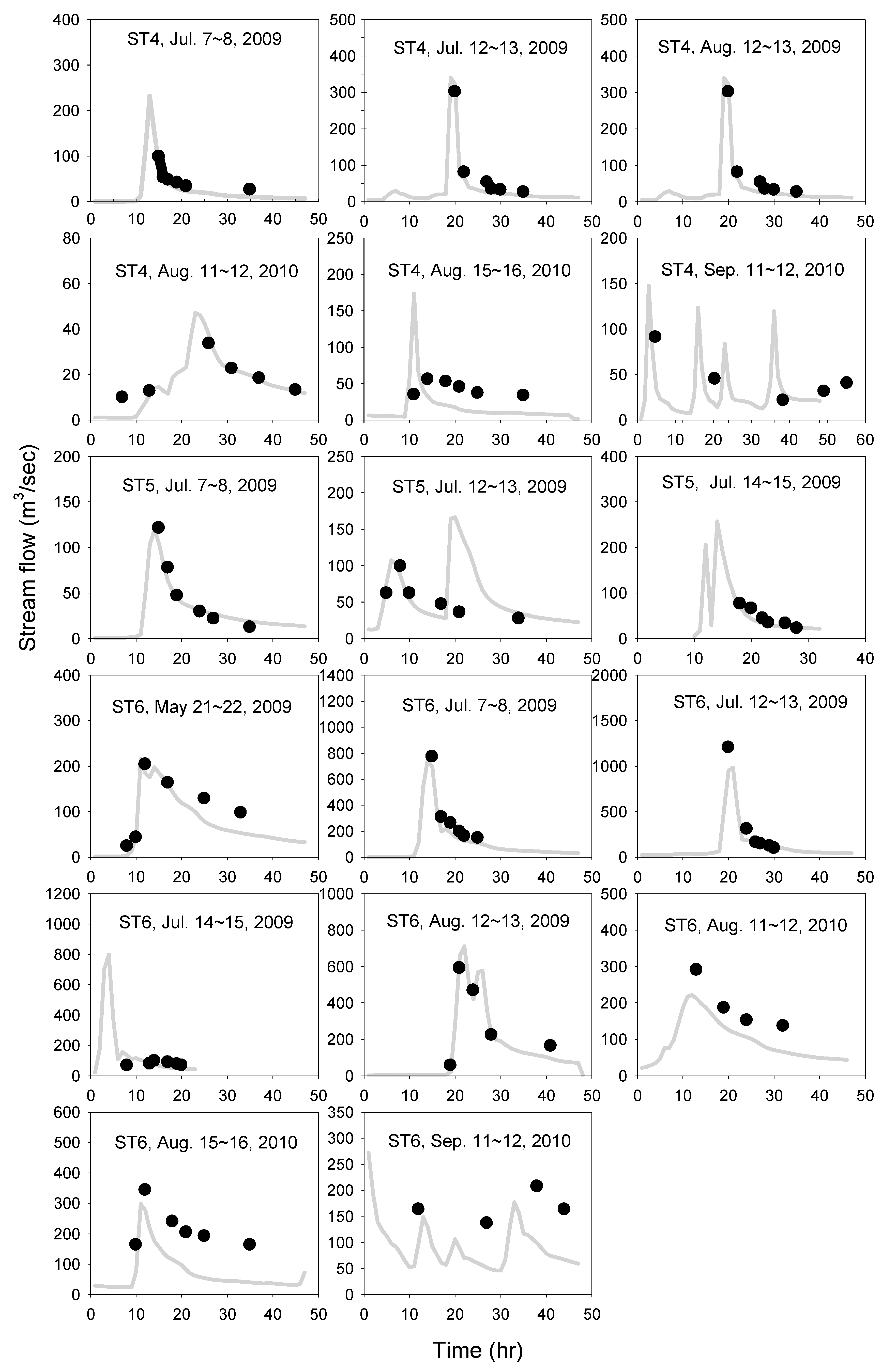
3.1. Calibration Results
3.2. Characteristics of Suspended Sediment Loadings under the East Asian Monsoon Climate
4. Conclusions
Acknowledgments
Author Contributions
Conflicts of Interest
References
- Park, S.; Oh, C.; Jeon, S.; Jung, H.; Choi, C. Soil erosion risk in Korea watersheds, assessed using the revised universal soil loss equation. J. Hydrol. 2011, 399, 263–273. [Google Scholar] [CrossRef]
- U.S. Environmental Protection Agency (EPA). EPA 841-B-99-004 Protocol for Developing Sediment TMDLs, 1st ed.U.S. EPA: Washington, DC, USA, 1999.
- Crabill, C.; Donald, R.; Snelling, J.; Foust, R.; Southam, G. The impact of sediment fecal coliform reservoirs on seasonal water quality in Oak Creek, Arizona. Water Res. 1999, 33, 2163–2171. [Google Scholar] [CrossRef]
- Somura, H.; Takeda, I.; Arnold, J.G.; Mori, Y.; Jeong, J.; Kannan, N.; Hoffman, D. Impact of suspended sediment and nutrient loading from land uses against water quality in the Hii River basin, Japan. J. Hydrol. 2012, 450–451, 25–35. [Google Scholar] [CrossRef]
- Renard, K.G.; Foster, G.R.; Weesies, G.A.; Porter, J.P. RUSLE: Revised universal soil loss equation. J. Soil Water Conserv. 1991, 46, 30–33. [Google Scholar]
- Meng, L.; Feng, Q.; Wu, K.; Meng, Q. Quantitave evalustion of soil erosion of land subsided by coal mining using RUSLE. Int. J. Min. Sci. Technol. 2012, 22, 7–11. [Google Scholar] [CrossRef]
- Nyakatawa, E.Z.; Jakkula, V.; Reddy, K.C.; Lemunyon, J.L.; Norris, B.E. Soil erosion estimation in conservation tillage systems with poultry litter application using RUSLE 2.0 model. Soil Tillage Res. 2007, 94, 410–419. [Google Scholar] [CrossRef]
- Fu, G.; Chen, S.; McCool, D.K. Modeling the impacts of no-till practice on soil erosion and sediment yield with RUSLE, SEDD, and ArcView GIS. Soil Tillage Res. 2006, 85, 38–49. [Google Scholar] [CrossRef]
- Neitsch, S.L.; Arnold, J.G.; Kiniry, J.R.; Williams, J.R. TR-406 Soil and Water Assessment Tool Theoretical Documentation Version 2009; Texas Water Resources Institute: College Station, TX, USA, 2011. [Google Scholar]
- Qiu, L.J.; Zheng, F.L.; Yin, R.S. SWAT-based runoff and sediment simulation in a small watershed, the loessial hilly-gullied region of China: Capabilities and challenges. Int. J. Sediment Res. 2012, 27, 226–234. [Google Scholar] [CrossRef]
- Oeurng, C.; Sauvage, S.; Sánchez-Pérez, J.M. Assessment of hydrology, sediment and particulate organic carbon yield in a large agricultural catchment using the SWAT model. J. Hydrol. 2011, 401, 145–153. [Google Scholar] [CrossRef] [Green Version]
- Sommerlot, A.R.; Nejadhashemi, A.P.; Woznicki, S.A.; Giri, S. Evaluating the capabilities of watershed-scale models in estimating sediment yield at field-scale. J. Environ. Manag. 2013, 127, 228–236. [Google Scholar] [CrossRef] [PubMed]
- U.S. Environmental Protection Agency (EPA). EAP841-B-97-006 Compendium of Tool for Watershed Assessment and TMDL Development; U.S. EPA: Washington, DC, USA, 1997.
- Ouyang, Y.; Leininger, T.D.; Moran, M. Impact of reforestation upon sediment load and water outflow in the Lower Yazoo River Watershed, Mississippi. Ecol. Eng. 2013, 61, 394–406. [Google Scholar] [CrossRef]
- Hunter, H.M.; Walton, R.S. Land-use effects on fluxes of suspended sediment, nitrogen and phosphorus from a river catchment of the Great Barrier Reef, Australia. J. Hydrol. 2008, 356, 131–146. [Google Scholar] [CrossRef]
- Benaman, J.; Shoemaker, C.A. An analysis of high-flow sediment event data for evaluating model performance. Hydrol. Process 2005, 19, 605–620. [Google Scholar] [CrossRef]
- Thompson, J.; Cassidy, R.; Doody, D.G.; Flynn, R. Assessing suspended sediment dynamics in relation to ecological thresholds and sampling strategies in two Irish headwater catchments. Sci. Total Environ. 2013, 468–469, 345–357. [Google Scholar] [CrossRef] [PubMed]
- Bicknell, B.R.; Imhoff, J.C.; Kittle, J.L.; Jobes, T.H.; Donigian, A.S. HSPF Version 12 User’s Manual; AQUA TERRA Consultants: Mountain View, CA, USA, 2004. [Google Scholar]
- Shin, M.J.; Eun, J.J.; Seo, E.W. Changes of gill structure and identification of genes by muddy water exposure in Cyprinus Carpio. Korean J. Limnol. 2011, 44, 95–101. [Google Scholar]
- Kim, S.H. Influence of Muddy Water in Imha Reservoir on the Community Fluctuation of Benthic Macroinvertebrates and Food Selection of Fishes. Master’s Thesis, Andong National University, Andong, Korea, 2009. [Google Scholar]
- U.S. Environmental Protection Agency (EPA). Basins Technical Note 6: Estimating Hydrology and Hydraulic Parameters for HSPF; U.S. EPA: Washington, DC, USA, 2000.
- U.S. Environmental Protection Agency (EPA). Basins Technical Note 8: Sediment Parameter and Calibration Guidance for HSPF; U.S. EPA: Washington, DC, USA, 2006.
- Donigian, A.S. Watershed Model Calibration and Validation: The HSPF Experience. In Proceedings of the National TMDL Science and Policy Specialty Conference 2002, Phoenix, AR, USA, 13–16 November 2002.
- Nash, J.E.; Sutcliffe, J.V. Reiver flow forecasting through conceptual model. Part 1. A discussion of principles. J. Hydrol. 1970, 10, 282–290. [Google Scholar] [CrossRef]
- Hsu, S.M.; Wen, H.Y.; Chen, N.C.; Hsu, S.Y.; Chi, S.Y. Using an integrated method to estimate watershed sediment yield during heavy rain period: A case study in Hualien County, Taiwan. Nat. Hazards Earth Syst. Sci. 2012, 12, 1949–1960. [Google Scholar] [CrossRef]
- Betrie, G.D.; Mohamed, Y.A.; van Griensven, A.; Srinivasan, R. Sediment management modeling in the Blue Nile Basin using SWAT model. Hydrol. Earth Syst. Sci. 2011, 15, 807–818. [Google Scholar] [CrossRef]
- Lenzi, M.A.; Marchi, L. Suspended sediment load during floods in a small stream of the Dolomites (northeastern Italy). CATENA 2000, 39, 267–282. [Google Scholar] [CrossRef]
- Saleh, A.; Du, B. Evaluation of SWAT and HSPF within BASINS program for the Upper North Bosque River Watershed in Central Texas. Trans. ASAE 2004, 47, 1039–1049. [Google Scholar]
- Lau, K.-M.; Yang, G.J.; Shen, S.H. Seasonal and intraseasonal climatology of summer monsoon rainfall over East Asia. Mon. Weather Rev. 1987, 116, 18–37. [Google Scholar] [CrossRef]
- Heo, S.G.; Kim, K.S.; Sagong, M.; Ahn, J.H.; Lim, K.J. Evaluation of SWAT applicability to simulate soil erosion at highland agricultural lands. J. Korean Soc. Rural Plan. 2005, 11, 67–74. [Google Scholar]


| Station ID | Area (km2) | Land Use (%) | ||||||
|---|---|---|---|---|---|---|---|---|
| Urban | Wetland | Agriculture | Forest | Water | Barren | Pasture | ||
| ST1 | 70.9 | 0.4 | 1.1 | 4.3 | 92.8 | 0.8 | 0.5 | 0.1 |
| ST2 | 11.4 | 8.5 | 5.4 | 26.2 | 58.2 | 0.8 | 0.5 | 0.4 |
| ST3 | 21.3 | 1.0 | 2.7 | 11.3 | 83.2 | 1.3 | 0.4 | 0.1 |
| ST4 | 144.3 | 1.0 | 3.4 | 10.6 | 83.2 | 1.3 | 0.4 | 0.1 |
| ST5 | 397.4 | 1.3 | 2.8 | 10.5 | 83.2 | 1.4 | 0.6 | 0.2 |
| ST6 | 537.9 | 1.6 | 2.8 | 11.3 | 81.4 | 1.5 | 0.9 | 0.5 |
| Date | Rainfall (mm) | Duration (h) | Maximum Rainfall Intensity (mm/h) | Calibrated Watershed |
|---|---|---|---|---|
| 21 May 2009 | 50.9 | 11 | 9.0 | ST1, ST2, ST3, ST6 |
| 2 July 2009 | 59.0 | 10 | 24.0 | ST1, ST2, ST3, ST4, ST5, ST6 |
| 12 July 2009 | 67.9 | 19 | 20.0 | ST1, ST3, ST4, ST5, ST6 |
| 15 July 2009 | 41.9 | 10 | 20.0 | ST1, ST3, ST5, ST6 |
| 11 August 2009 | 72.9 | 14 | 16.0 | ST1, ST4, ST6 |
| 23 May 2010 | 59.8 | 44 | 6.0 | ST2 |
| 12 August 2010 | 28.0 | 4 | 16.0 | ST1, ST2, ST3, ST4, ST6 |
| 15 August 2010 | 31.0 | 5 | 20.0 | ST1, ST4, ST5, ST6 |
| 11 September 2010 | 68.9 | 40 | 21.0 | ST2, ST3, ST4, ST6 |
| Parameter | Ranges | |||||
|---|---|---|---|---|---|---|
| Upland | Forest | Pasture | Barren | Urban | ||
| Water budget | LZSN (cm) | 4.1–20.3 | 3.8–18.8 | 4.1–20.3 | 3.8–18.8 | |
| INFILT (cm/h) | 2.0–13.0 | 1.4–9.2 | 2.0–13.6 | 2.5–23.4 | ||
| UZSN (cm) | 0.2–4.1 | 0.2–5.1 | 0.2–4.1 | 0.1–3.0 | ||
| NSUR | 0.03–0.3 | 0.04–0.5 | 0.03–0.3 | 0.02–0.3 | 0.01–0.1 | |
| AGWRC (/day) | 0.833–0.999 | |||||
| IRC (/day) | 0.3–0.85 | |||||
| INTFW (/day) | 1.0–10.0 | |||||
| DEEPER | 0.0–0.5 | |||||
| BASETP | 0.0–0.05 | |||||
| Sediment | KRER | 0.05–0.75 | ||||
| JRER | 1.0–3.0 | |||||
| AFFIX | 0.01–0.50 | |||||
| KSER | 0.1–10.0 | |||||
| JSER | 1.0–3.0 | |||||
| KGER | 0.0–10.0 | |||||
| JGER | 1.0–5.0 | |||||
| Calibration Item | Very Good | Good | Fair | Poor | |
|---|---|---|---|---|---|
| Daily Stream flow | R2 | >0.8 | 0.7–0.8 | 0.6–0.7 | <0.6 |
| Sediment | RE (%) | <20 | 20–30 | 30–45 | >45 |
| Calibration Item | ST1 | ST2 | ST3 | ST4 | ST5 | ST6 | |
|---|---|---|---|---|---|---|---|
| Stream flow | R2 | 0.80 | 0.76 | 0.95 | 0.86 | 0.89 | 0.93 |
| NS | 0.88 | 0.78 | 0.95 | 0.89 | 0.96 | 0.86 | |
| Suspended Sediment yields | R2 | 0.87 | 0.96 | 0.90 | 0.60 | 0.89 | 0.62 |
| RE (%) | 23 | −1 | 22 | −14 | −13 | 16 | |
| Parameter | Ranges | |||||
|---|---|---|---|---|---|---|
| Upland | Forest | Pasture | Barren | Urban | ||
| Water budget | LZSN (cm) | 7.7–16.1 | 7.58–8.96 | 5.08–13.83 | 7.19–18.75 | |
| INFILT (cm/h) | 0.18–0.20 | 0.13 | 0.04–0.54 | 0.22–0.46 | ||
| UZSN (cm) | 0.19–0.23 | 0.25–0.26 | 0.17–0.26 | 0.13–0.26 | ||
| NSUR | 0.21–0.34 | 0.37 | 0.11–0.25 | 0.05–0.27 | 0.05 | |
| AGWRC (/day) | 0.88–0.91 | |||||
| IRC (/day) | 0.40 | |||||
| INTFW | 1.97–2.01 | |||||
| DEEPER | 0.45 | |||||
| BASETP | 0.02 | |||||
| Sediment | KRER | 0.05–0.40 | ||||
| JRER | 1.00–2.57 | |||||
| KSER | 0.10–2.00 | |||||
| JSER | 2.00–3.00 | |||||
| KGER | 0.0001–1.70 | |||||
| JGER | 2.50–5.00 | |||||
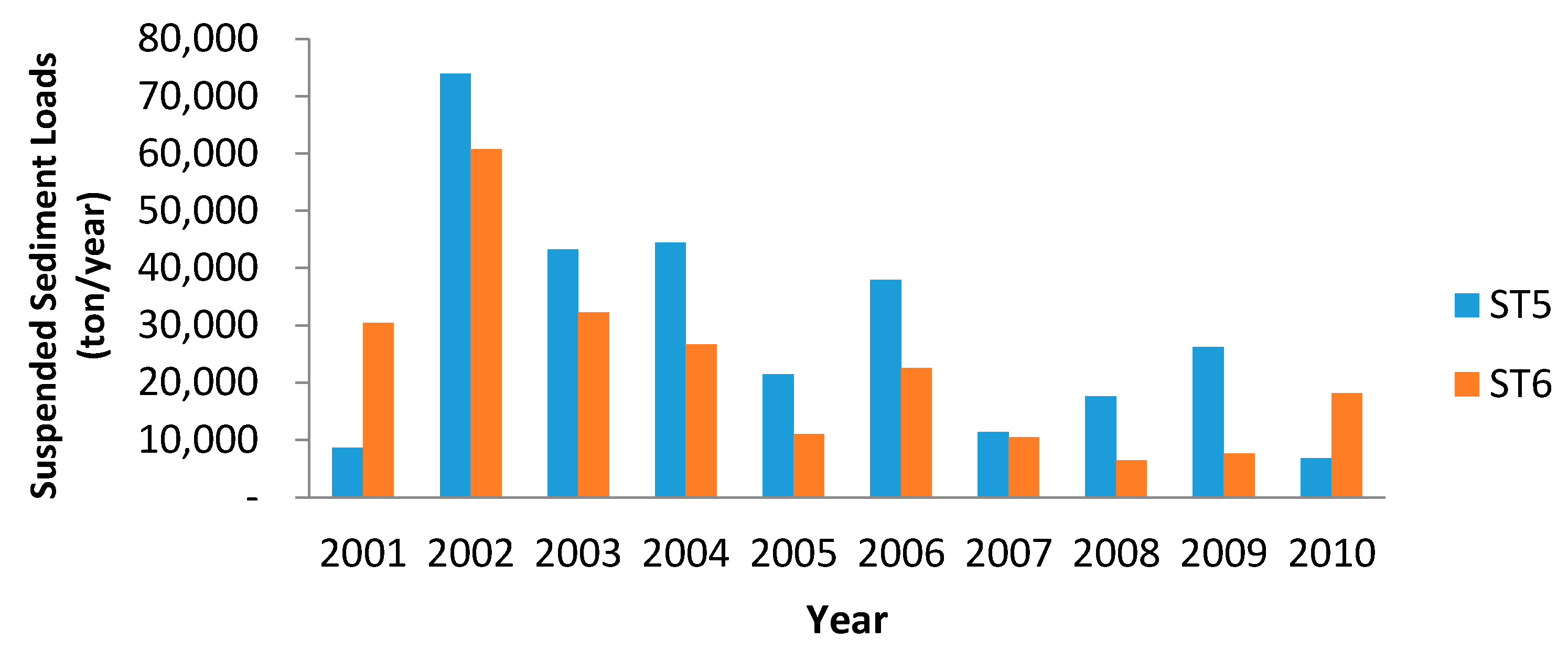
| Station ID | Average | Maximium | Minimum | Max/Min * | STD ** |
|---|---|---|---|---|---|
| ST5 | 29,187 | 73,955 | 6873 | 11 | 19,869 |
| ST6 | 22,646 | 60,787 | 6454 | 9 | 15,527 |
| Year | ST5 | ST6 | ||||
|---|---|---|---|---|---|---|
| Yearly * | Event ** | Ratio *** | Yearly | Event | Ratio | |
| 2001 | 8711 | 4090 | 0.47 | 30,398 | 20,205 | 0.66 |
| 2002 | 73,955 | 37,283 | 0.50 | 60,787 | 25,202 | 0.41 |
| 2003 | 43,284 | 11,085 | 0.26 | 32,210 | 10,233 | 0.32 |
| 2004 | 44,412 | 16,575 | 0.37 | 26,666 | 9714 | 0.36 |
| 2005 | 21,473 | 17,076 | 0.80 | 11,038 | 5420 | 0.49 |
| 2006 | 37,953 | 29,353 | 0.77 | 22,554 | 20,260 | 0.90 |
| 2007 | 11,409 | 5339 | 0.47 | 10,537 | 3019 | 0.29 |
| 2008 | 17,579 | 16,465 | 0.94 | 6454 | 3676 | 0.57 |
| 2009 | 26,222 | 18,213 | 0.69 | 7661 | 4447 | 0.58 |
| 2010 | 6873 | 2922 | 0.43 | 18,149 | 12,504 | 0.69 |
| Average | 29,187 | 15,840 | 0.54 | 22,646 | 11,468 | 0.51 |
© 2016 by the authors; licensee MDPI, Basel, Switzerland. This article is an open access article distributed under the terms and conditions of the Creative Commons Attribution (CC-BY) license (http://creativecommons.org/licenses/by/4.0/).
Share and Cite
Jeon, J.-H.; Park, C.-G.; Choi, D.; Kim, T. Characteristics of Suspended Sediment Loadings under Asian Summer Monsoon Climate Using the Hydrological Simulation Program-FORTRAN. Sustainability 2017, 9, 44. https://doi.org/10.3390/su9010044
Jeon J-H, Park C-G, Choi D, Kim T. Characteristics of Suspended Sediment Loadings under Asian Summer Monsoon Climate Using the Hydrological Simulation Program-FORTRAN. Sustainability. 2017; 9(1):44. https://doi.org/10.3390/su9010044
Chicago/Turabian StyleJeon, Ji-Hong, Chan-Gi Park, Donghyuk Choi, and Taedong Kim. 2017. "Characteristics of Suspended Sediment Loadings under Asian Summer Monsoon Climate Using the Hydrological Simulation Program-FORTRAN" Sustainability 9, no. 1: 44. https://doi.org/10.3390/su9010044