Electricity Consumption and Economic Growth: Evidence from 17 Taiwanese Industries

Abstract

The current paper investigates the existence and nature of the Granger causality between electricity consumption and economic growth for 17 industries in Taiwan. Empirical results over the period 1998–2014 suggest that a panel cointegration test shows a long-run equilibrium relationship and a bi-directional Granger causality between electricity and economic growth has been found. The result indicates that a 1% increase in electricity consumption boosts the real GDP by 1.72%. The government can pursue energy conservation and carbon reduction policy in some industries without impeding the economic growth for adjusting the industrial structure.

1. Introduction

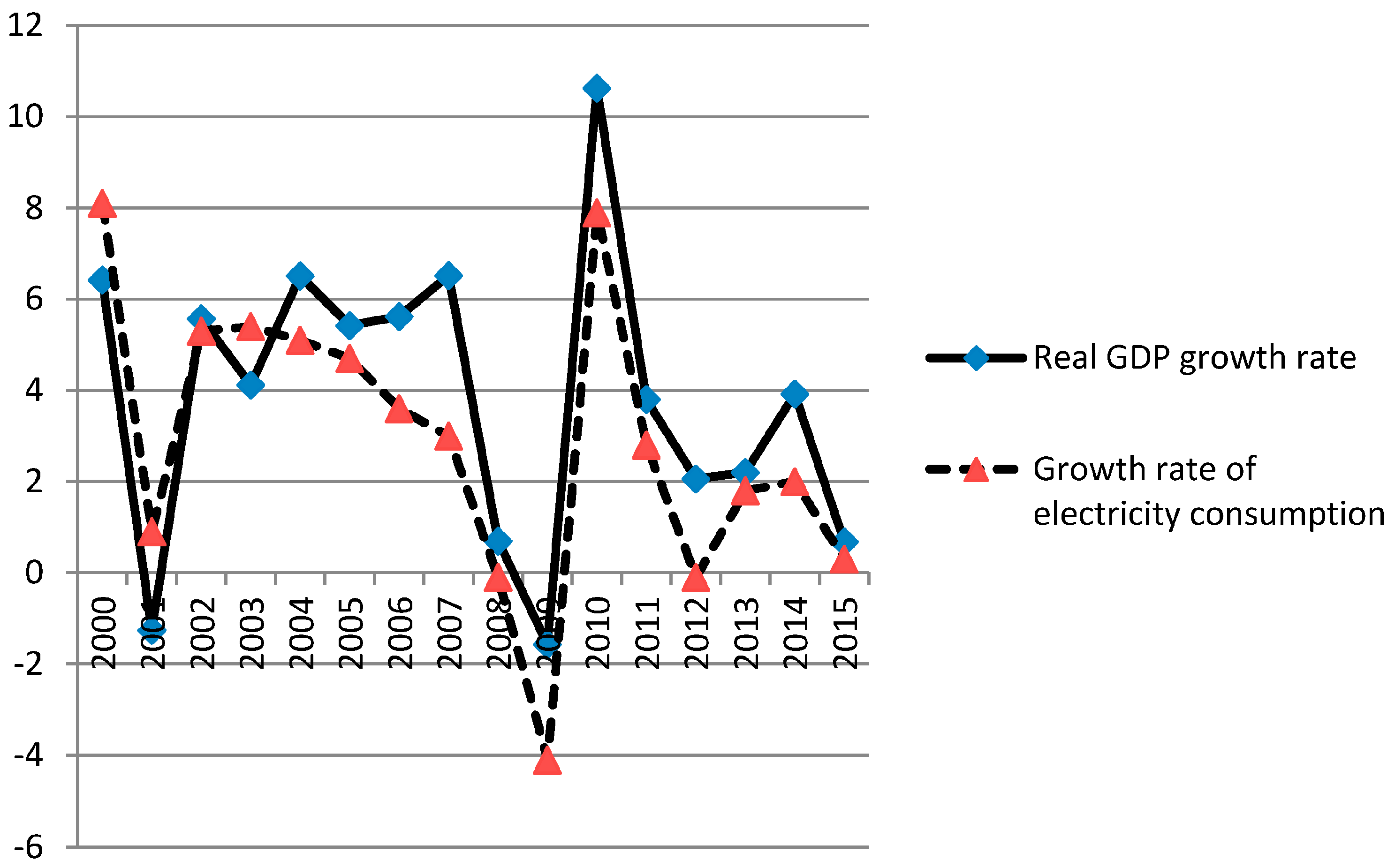
In the recent decades policymakers have been mitigating global warming and climate change. Paris climate conference (COP21) was held in December 2015, the goal of which was to affirm the goal of limiting global temperature increase below 2 degrees Celsius above the pre-industrial levels. Parties of the Paris climate conference also ascertained the need to report how well they are doing in terms of implementing their targets and tracking their progress toward the long-term goal through a robust, transparent, and accountable system. However, the design of such energy-saving policies has a significant impact on economic growth. Since the seminal work of Kraft and Kraft [1], many studies have investigated the causal relationship between energy or electricity consumption and economic growth. On an aggregate or national level, electricity consumption is strongly related with economic growth (see, for example, [2,3,4,5,6,7,8,9,10,11,12,13,14,15,16,17,18,19,20]). As previous studies have suggested, economic growth depends highly on energy inputs. Taiwan is a developing country whose manufacturing industry relies heavily on energy consumption. In Figure 1, the dotted line represents the growth rate of electricity consumption and the solid line represents the real GDP growth rate in Taiwan. Clearly, electricity consumption is highly correlated with the growth of real GDP. Therefore, the relationship between electricity consumption and GDP growth is worth investigating.

Most existing studies have investigated the relationship between electricity consumption and economic growth using national or aggregate data. However, support for the energy–growth nexus does not imply the existence of this relationship at the industrial level, even though some industries may exhibit intensive use of energy. It would, thus, be worthwhile to study the link between electricity consumption and economic growth at the industry level. Such an analysis could help us identify specific energy conservation policy and carbon reduction techniques for energy intensive industries. This paper explores the relationship between the real GDP growth and electricity consumption at the industry level during the time period 1998–2014.

This paper also distinctly contributes to the existing literature. First of all, this research sheds new light on the electricity consumption and real GDP growth at an industrial level. Reviewing the existing literature, most studies focus on the energy–growth dynamics using aggregate or national-level data that led to conflicting results. As Soytas et al. [21] argued, disaggregated level data may provide further insight regarding the link between real GDP and energy consumption. Thus, we feel the use of industrial data may elicit the correct diagnosis of the energy–GDP nexus. Second, the relationship between electricity consumption and the real GDP growth may differ from industry to industry. We can observe the heterogeneous effects of energy policy on various industries.

In this paper, we extend research in this field by using data from 17 Taiwanese industries for the years 1998–2014. The results can be summarized as follows:

(1)

We find that electricity consumption and real industrial GDP are both integrated of order one. The findings of the Westerlund [22] cointegration test reveal that the two variables are cointegrated.

(2)

Applying the dynamic ordinary least squares method (hereafter, DOLS) to estimate the long-run equilibrium equation, we found that, in the mining and quarrying and wholesale trade industries, electricity consumption has a negative impact on GDP growth. Hence, the energy policy makers can safely adopt the energy (electricity) conservation policy without hindering the GDP growth. However, most of the panel DOLS test results in the current research indicate that electricity consumption has a positive impact on economic growth. A 1% increase in electricity consumption leads to a 1.72% increase in economic growth. The long-run relationship suggests the existence of a positive relationship between the two variables.

(3)

The short- and long-run Granger causality tests were examined and we discovered the existence of a bidirectional causal relationship between the real GDP growth and electricity consumption in the short- and long-run. The results imply that the reduction in energy or electricity consumption may adversely affect economic growth.

The remaining paper is organized as follows: Section 2 gives an overview of the existing literature; Section 3 discusses the proposed econometric model; Section 4 lists the empirical results; Section 5 concludes the research and provides policy implications.

2. Literature Review

Energy consumption plays an important role in economic growth. Kraft and Kraft [1] were the first ones to investigate the relationship between energy consumption and economic growth by using various econometric methods for different time periods. From an economist’s perspective, energy is an input for production but empirical evidence suggests that the energy-growth nexus is complicated. Most empirical studies employ the cointegration and Granger causality model (summarized in

Table 1. Summary of empirical results.

Authors	Method	Data Period	Results	Countries or Industries
Abdoli et al. [2]	Panel cointegration and FMOLS estimation	1980–2011	Energy consumption$\to$GDP (short-run causality) Electricity$\leftrightarrow$GDP (long-run causality)	OECD countries
Apergis and Payne [16]	Dynamic panel data model and causality test	1990–2007	In the short-run: Electricity$\leftrightarrow$GDP (in high- and upper-middle-income countries); Electricity$\to$GDP (in low-income countries. In the long-run: Electricity$\leftrightarrow$GDP (in lower-middle, high- and upper-middle-income states)	Four types countries: High-income countries, upper-middle-income countries, lower-middle countries, and low-income countries
Aslan [3]	ARDL bound test and Granger causality test	1968–2008	Electricity$\leftrightarrow$GDP	Turkey
Bayar [4]	Panel cointegration and a Granger causality test	1970–2011	Electricity$\leftrightarrow$GDP	21 emerging countries
Chang [5]	VECM, Cointegration and Granger Causality test	1981–2006	Electricity$\leftrightarrow$GDP	China
Chen et al. [6]	Johansen’s cointegration test and panel causality test	1971–2001	GDP$\to$Energy consumption (in the short-run causality); Electricity$\leftrightarrow$GDP (in the long-run causality)	10 developing Asian countries
Jumbe [12]	Granger causality and Error-correction model	1970–1999	Electricity$\leftrightarrow$GDP	Malawi
Li et al. [29]	Cointegration and DOLS estimation	1985–2007	Electricity$\leftrightarrow$GDP	30 provinces in China
Nazlioglu et al. [8]	Bound testing, Cointegration, linear and nonlinear Granger causality test	1967–2007	Electricity$\leftrightarrow$GDP (linear Granger causality); There was no causality between electricity and GDP (nonlinear Granger causality)	Turkey
Ogundipe and Apata [10]	Johansen Cointegration test and Granger causality test	1980–2008	Electricity$\leftrightarrow$GDP	Nigeria
Shahbaz and Feridun [11]	ARDL bounds test and Toda Yamamoto causality test	1971–2008	GDP$\to$Electricity	Pakistan
Wolde-Rufael [9]	Granger causality test (Toda and Yamamoto’s method) and cointegration test	1971–2001	Electricity$\to$GDP (Benin, Congo, Egypt, Morocco, Gabon, Tunisia); GDP$\to$Electricity (Cameroon, Ghana, Zimbabwe, Zambia, Nigeria, Senegal); No causality (Algeria, Kenya, South Africa, Sudan)	17 African countries
Yuan et al. [19]	VECM, Cointegration and Granger Causality test	1990–2005	Electricity$\to$GDP Oi consumption$\leftrightarrow$GDP; GDP$\to$Coal consumption	China
Yoo [17]	Error-correction model	1970–2002	Electricity$\leftrightarrow$GDP	Korea
Yoo [18]	Hsiao’s Granger causality test	1971–2002	Electricity$\leftrightarrow$GDP (Malaysia and Singapore); $\mathrm{GDP}\to$Electricity (Thailand and Indonesia)	ASEAN 4 countries
Zhang and Cheng [20]	VAR and Granger Causality test	1960–2007	GDP$\to$Energy consumption	China

Note: A$\to$B, and A$\leftrightarrow$B denote causality runs from A to B and a bi-directional causality runs between A and B, respectively.

). The previous test results are based on the time series economic analysis and dynamic panel data approach. Electricity consumption and the real GDP are often non-stationary and take some cointegration tests into account. However, the two variables reveal conflicting results on the issue at hand because the estimation results are very sensitive to the time period considered and the methodology employed. Another factor contributing to the complications of the energy-growth nexus is the difference in the region where the study was conducted (see, for example, [2,3,4,5,6,7,8,9,10,11,12,13,14,15,16,17,18,19,20]). These studies mostly focus on the developed and developing countries; however, they do not reach a consensus on the role of energy in economic development. Turning to different data sets, it is important to take data properties into consideration as methods and empirical results depend on whether the data is suitable for conducting an empirical analysis. Most of the empirical research has used aggregated or national-level data to analyze this issue. Soytas and Sari [23] argued that many works suffer from aggregate bias. Campbell and Perron [24] reported that the relatively short time span may substantially weaken the power of statistics test, thereby producing distorted and mixed results. National-level data fails to address the heterogeneous effects of the issue. In this paper, we investigate the industrial nexus and address the abovementioned effects for different industries.

To the best of our knowledge, few empirical studies study the energy-GDP issue based on industry-level data. Xu and Pan [25], Zhang and Xu [26] and Hu and Wang [27] examined the relationship between energy consumption and economic growth in sectors and regions in China. Hamit-Haggar [28] applied time series econometric analysis and dynamic panel data methods to investigate the relationship between energy consumption and economic growth for Canadian industrial sectors. Xu and Pan [25] discovered a long-term equilibrium relationship between the energy consumption of the six big industries and their industrial growth. Zhang and Xu [26] found that economic growth involves more energy consumption at the sectoral levels. The industries in the eastern region of China showcase a bidirectional causality relationship between energy consumption and economic growth. Hamit-Haggar [28] showed that there exists a short-run Granger causality running from energy consumption to economic growth and that the environmental Kuznets curve holds. Hu and Wang [27] revealed that a 1% increase in energy consumption increases the real value added of industrial sectors by 0.871% and a 1% increase in value added of industrial sectors boosts energy consumption by 1.103%. They found a unidirectional causation from economic growth to energy consumption. However, energy consumption is found to cause economic growth in the long run.

Due to great differences in energy consumption observed across industries, it would be worthwhile to study the relationship between energy consumption and economic growth at the industry level. Conducting this research will be helpful in designing a more efficient energy conservation, emission reduction policy and in making adjustment for the industrial structure. In this paper, we focus on this issue in the context of 17 industries by employing empirical analysis.

3. Econometric Analysis

In an attempt to give clear proof of the short-run and long-run link between electricity consumption and economic growth, the paper makes use of the Taiwanese annual panel data from 1998 to 2014. The data used in the study includes electricity consumption and real GDP at the industry level. These variables are then expressed in a natural logarithmic form. Many previous empirical studies used aggregated data and measures focused on the relation between energy (electricity) consumption and economic growth both in the developed and developing countries. Soytas and Sari [23] pointed out that many issues might suffer from aggregation bias. A few studies shed light on disaggregate or section-specific energy/electricity consumption and its contribution to GDP. Sector-specific data can address the heterogeneous effects of energy conservation policies on different sectors with different energy usage intensities. For the purpose of investigating the link between industrial electricity consumption and growth, the study uses the following procedures. First, the unit root test is carried out by employing the Im, Pesaran, and Shin unit root test [30]. The results of the test determine the stationarity properties and the order of integration. Second, we adopted Westlung [22] panel cointegration tests to examine the cointegration relationship between sector-specific energy consumption and economic growth. Finally, we examine the short- and long-run causal relation between energy consumption and economic growth.

3.1. Panel Unit Root Test

To confirm the integration order of variables, we start by performing a unit root test. The traditional univariate unit-root tests, initiated by Dickey and Fuller, have low power problems and it becomes difficult to reject the null hypothesis. Because of the weakness of the univariate unit root test, we conduct the Im, Pesaran and Shin [30] unit root test (hereafter, IPS) (Pesaren [31] have detailed discussed in detail the IPS standardized statistics and asymptotical distribution.) which is based on panel data. The IPS test is less restrictive and more powerful compared to the traditional ADF test (for a useful survey on panel unit root test, see Hurlin and Mignon [32]). The basic equation for the panel unit root tests for IPS is as follows:

$$\Delta y_{i,t}={\alpha }_i+{\rho }_i{y}_{i,t}+{\sum }_{j=1}^p{\phi }_{ij}\Delta y_{i,t-j}+{\epsilon }_{i,t};i=1,2,\dots ,N;t=1,2,\dots ,T$$

(1)

where $y_{i,t}$ represents each variable under consideration in our model, ${\alpha }_i$ is the individual fixed effect, and $p$ is selected to make the residuals uncorrelated over time. The null hypothesis is that all panels contain unit roots (${\rho }_i=0,\forall alli$) versus the alternative hypothesis that at least one panel is stationary (${\rho }_i<0$ for some $i=1,2,\dots ,N_1$ and ${\rho }_i=0$ for $i=N_1+1,\dots ,N$). The IPS statistic is based on averaging individual ADF statistics and can be written as $\overline{t}=\frac{1}{N}{\sum }_{i=1}^N{t}_{i,T}$, where $t_{i,T}$ is the ADF t-statistic for industry $i$ based on the sector-specific ADF regression. IPS shows that under the null hypothesis of non-stationary, the $\overline{t}$ statistic follows the standard normal distribution asymptotically. The standardized statistic $t_{IPS}$ is expressed as:

$$t_{IPS}=\frac{\sqrt{N\left[\overline{t}-E\left(t_i\right)\right]}}{\sqrt{Var\left(t_i\right)}}$$

(2)

The limitation of the IPS test is that it is cross-section-dependent, potentially because of unobserved common factors and externalities, as well as regional and macroeconomic linkages. Thus, some new panel unit root tests, addressing cross-section dependence, have been reported. A well-known test, considering cross-section dependence, is the CIPS test of Pesaran [33], where the following cross-sectional augmented Dickey-Fuller (CADF) regression is considered and the OLS method for the ith cross-section in the panel is estimated:

$$\Delta y_{i,t}={\alpha }_i+{\rho }_i{y}_{i,t}+{\delta }_i{\overline{y}}_{t-1}+{\sum }_{j=0}^k{\delta }_{ij}\Delta {\overline{y}}_{i,t-j}+{\sum }_{j=0}^k{\phi }_{ij}\Delta y_{i,t-j}+{ϵ}_{i,t}$$

(3)

where ${\overline{y}}_{t-1}=\frac{1}{N}{\sum }_{i=1}^N{y}_{i,t-1}$ and $\Delta {\overline{y}}_t=\frac{1}{N}{\sum }_{i=1}^N\Delta y_{i,t}$. Pesaran [33] proposes a cross-sectional augmented version of the IPS test:

$$\mathrm{CIPS}=\frac{1}{N}{\sum }_{i=1}^{N}CAD{F}_i$$

(4)

where $CAD{F}_i$ is the CADF statistic for the ith cross-sectional unit given by the t statistic of the estimate of ${\rho }_i$.

These results strongly suggest that the variables are nonstationary and level but stationary in first differences; they may be integrated of the first order $\mathrm{I}\left(1\right)$. In such cases, the presence of a cointegration relationship between the series can be examined because the considered integrated series are of the same order. Thus, the results of the CIPS test, considering cross-sectional dependence, are similar to those of the IPS test.

3.2. Panel Co-Integration Test

In recent years, it has become increasingly popular to use panel data sets for carrying out an econometric analysis. The long-run dimension in panel time series allows us to estimate the long-run relationship between variables by exploring regular time series analytical tools, such as the cointegration test and the causality relationship. In spite of this, we apply four panel cointegration tests developed by Westerlund [22] to test the cointegration relationship. (Banerjee, Dolado, and Mestre [34] and Kremers, Ericsson and Dolado [35] mentioned that, due to common-factor restriction low power problems for residual-based cointegration tests, many studies fail to reject the no-cointegration null, even in cases where cointegration is strongly suggested by theory. Westerlund [22] provided four new panel cointegration tests that are based on structural rather than residual dynamics and, therefore, do not impose any common-factor restriction.) The four tests are all normally distributed, while also being general enough to accommodate unit-specific short-run dynamics, unit-specific trends, and cross-sectional dependence.

The relationship between energy consumption and economic growth is as follows:

$$G_{i,t}={\mu }_i+{\beta }_i{E}_{i,t}+{\epsilon }_{i,t}$$

(5)

where $G_{i,t}$ is real GDP and $E_{i,t}$ is electricity consumption by industries. All series are transformed into logarithms. Based on Equation (5), the error correct model can be presented as follows:

$$\Delta G_{i,t}={\delta }_i^{\prime }{d}_t+{\alpha }_i\left(G_{i,t-1}-{\beta }_i^{\prime }{E}_{i,t-1}\right)+{\sum }_{j=1}^{p_i}{\phi }_{ij}\Delta G_{i.t-j}+{\sum }_{j=-q_i}^{p_i}{\gamma }_{ij}\Delta E_{i,t-j}+e_{i,t}$$

(6)

where $d_t={(1,t)}^{\prime }$, the parameter ${\alpha }_i$ provide estimates of the speed of error-correction toward the long-run equilibrium. ${\alpha }_i<0$ implies that $G_{i,t}$ and $E_{i,t}$ are cointegrated; if ${\alpha }_i=0$, then there is no error correction. We can depict the null hypothesis of no cointegration as $H_0:{\alpha }_i=0$ for all i. The alternative hypothesis depends on what is being assumed about the homogeneity of ${\alpha }_i$. According to Westerlund [22] and Persyn and Westerlund [36], group-mean tests, which do not require the ${\alpha }_i$s to be equal, imply that $H_0$ is tested versus $H_1^g:{\alpha }_i<0$ for at least one i. The statistic of group-mean tests can be computed in the following way:

$$D_{\tau }=\frac{1}{N}{\sum }_{i=1}^N\frac{\widehat{{\alpha }_i}}{SE\left({\widehat{\alpha }}_i\right)}$$

(7)

$$D_{\alpha }=\frac{1}{N}{\sum }_{i=1}^N\frac{T\widehat{{\alpha }_i}}{{\widehat{\alpha }}_i^{*}}$$

(8)

The other pair of tests of Westerlund [22] and Persyn and Westerlund [36] are called panel tests, and they assume that ${\alpha }_i$ is equal for all i, and are designed to test $H_0$ versus $H_1^p:{\alpha }_i=\alpha <0$ for all i. The panel statistics are as follows:

$$P_{\tau }=\frac{\widehat{\alpha }}{SE\left(\widehat{{\alpha }_i}\right)}$$

(9)

$$P_{\alpha }=\mathrm{T}\widehat{\mathsf{\alpha }}$$

(10)

By applying an error-correction model in which all variables are assumed to be I(1), the four tests proposed by Westerlund [22] examine whether cointegration is present or not by determining whether error-correction is present for individual panel members and for the panel as a whole.

3.3. Panel Dynamic Ordinary Least Squares

The DOLS method of Stock and Watson [37] is widely used to estimate and test hypotheses about a cointegrating vector to panel data. Kao and Chiang [38] and McCoskey and Kao [39] have precisely discussed the DOLS estimators. These authors note that the panel DOLS is less biased compared with other estimators in small samples that use Monte Carlo simulations. The panel DOLS estimators have better sample properties than the panel ordinary least squared estimators. The DOLS is obtained from the following equation:

$$G_{i,t}=d_i+E_{i,t}{\beta }_i+{\sum }_{j=-q}^q{C}_{i,j}\Delta E_{i,t+j}+{\epsilon }_{i,t}$$

(11)

where $C_{ij}$ is the coefficient of a lead or lag of first differenced explanatory variables. The estimated coefficient of DOLS is given by:

$${\widehat{\beta }}_{DOLS}={\sum }_{i=1}^N{\left({\sum }_{t=1}^T{Z}_{i,t}{Z}_{i,t}^{\prime }\right)}^{-1}\left({\sum }_{t=1}^T{Z}_{i,t}{\widehat{y}}_{i,t}^{+}\right)$$

(12)

where $Z_{i,t}=\left[\begin{array}{ccc}{E}_{i,t}-\overline{E_i},& \Delta E_{i,t-q},\dots ,& \Delta E_{i,t+q}\end{array}\right]$, ${\widehat{y}}_{i,t}^{+}$ is the transformed variable of $y_{i,t}$ to achieve the endogeneity correction. Kao and Chiang [38] show that the limited distribution of the DOLS estimators in cointegrated regressions are asymptotically normal.

We employ the panel DOLS method to estimate coefficients of the long-run relationship between electricity consumption and economic growth. Economists have long been interested in understanding the link between electricity consumption and economic growth for at least two reasons. First, knowing the relationship between electricity consumption and economic growth helps in determining the energy and economic development policy. The government can account for the different electricity consumption and needs to forecast future business conditions and uplift the status. Second, knowing the relation between electricity consumption and economic growth assists in identifying their causal relationship and establishing tax policy. For example, if electricity consumption would leave economic growth unaffected, increasing energy tax rate would not hurt economic growth.

3.4. Panel Granger Causality Tests

After examining the existences of cointegration, the direction of the causality relationship between the variables needs to be identified. The panel cointegration test confirms the long-run relationship exists between the variables. We test for causality relationship of the two variables. According to the Granger representation theorem, the panel vector error correction model can be constructed as follows:

$$\Delta G_{i,t}={\mu }_{1i}+{\sum }_{j=1}^p\Delta G_{i,t-j}{\beta }_{1j}+{\sum }_{j=1}^q\Delta E_{i,t-j}{\gamma }_{1j}+{\tau }_{1}EC{T}_{1,it-1}+{\epsilon }_{1,it}$$

(13)

$$\Delta E_{i,t}={\mu }_{1i}+{\sum }_{j=1}^p\Delta G_{i,t-j}{\beta }_{2j}+{\sum }_{j=1}^q\Delta E_{i,t-j}{\gamma }_{2j}+{\tau }_{2}EC{T}_{2,it-1}+{\epsilon }_{2,it}$$

(14)

in which, $\Delta$ denotes first differencing, and $EC{T}_{1,it-1}$ and $EC{T}_{2,it-1}$ are error correction terms. The lag length is chosen optimally using the AIC criterion. The error-correction model to be estimated by the pooled mean-group method (PMG) was suggested by Pesaran, Shin, and Smith [40,41]; here, we use the PMG estimator to estimate Equations (13) and (14) and evaluate two Granger causality relationships.

The researchers can test the significance of coefficients in Equations (13) and (14) to identified the sources of causation. In short-run causality, the significance of the coefficients related to the lagged difference of electricity consumption in Equation (13), and the real GDP in Equation (14) is evaluated. Long-run causality is related to the coefficient of ECT. The null hypothesis for short- and long-run Granger causality tests can be presented as follows:

(1)

Short-run Granger causality:

$H_0:{\gamma }_{1j}=0,\forall j=1,\dots ,q,\mathrm{in}\mathrm{Equation}\left(13\right)$

$H_0:{\beta }_{2j}=0,\forall j=1,\dots ,p,\mathrm{in}\mathrm{Equation}\left(14\right)$

(2)

Long-run Granger causality:

$H_0:{\tau }_1=0,\forall j=1,\dots ,q,\mathrm{in}\mathrm{Equation}\left(13\right)$

$H_0:{\tau }_2=0,\forall j=1,\dots ,q,\mathrm{in}\mathrm{Equation}\left(14\right)$

The panel causality test results will discuss in next section. We inferred a bidirectional causal relation between real GDP growth and electricity consumption in the short-run. The coefficient of ECT was significant in both Equations (13) and (14), suggesting bidirectional causality between electricity consumption and real GDP growth in the long-run.

4. Data and Empirical Results

4.1. Data

The electricity consumption data of 17 industries is taken from the industrial energy consumption of Taiwan Power Company [42] for the period 1998–2014. The Directorate General of Budget Accounting and Statistics in Taiwan annually publishes a National Accounts Yearbook and provides statistics data for the annual balance of real gross domestic products categorized according to the type of industrial activity since 1981. The real gross domestic products for all kinds of industries have been measured at 2006 constant prices and taken from the Directorate General of Budget Accounting and Statistics in Taiwan. Following the previous studies, we use industry level real gross domestic product to calculate the economic growth rate. All variables are expressed in the form of natural logarithms.

Table 2. Basic statistics.

Variables	Real GDP (${\mathit{G}}_{\mathit{i}}$)				Energy Consumption (${\mathit{E}}_{\mathit{i}}$)
	Mean	Standard Deviation	Maximum	Minimum	Mean	Standard Deviation	Maximum	Minimum
Mining and Quarry	9.93	0.35	10.55	9.43	19.80	0.15	20.02	19.50
Beverages, and Tobacco Manufacturing	12.01	0.08	12.12	11.89	21.92	0.09	22.06	21.77
Textiles Mills Manufacturing	10.59	0.37	11.24	10.16	20.17	0.12	20.34	19.99
Wearing Apparel and Clothing Accessories Manufacturing	9.83	0.12	10.01	9.63	19.43	0.12	19.59	19.20
Wood and Bamboo Products Manufacturing	9.31	0.11	9.47	9.06	19.59	0.13	19.82	19.41
Pulp, Paper and Paper Products Manufacturing	10.79	0.11	10.95	10.57	21.47	0.06	21.57	21.35
Chemical Material Manufacturing	12.34	0.31	12.77	11.78	22.67	0.03	22.70	22.61
Chemical Products Manufacturing	10.67	0.27	11.08	10.31	21.72	0.15	21.94	21.36
Non-metallic Mineral Products Manufacturing	11.32	0.38	11.93	10.91	22.24	0.14	22.44	22.04
Basic Metal Manufacturing	12.22	0.23	12.69	11.89	23.12	0.13	23.28	22.89
Electronic Parts and Components Manufacturing	13.16	0.82	14.29	11.71	23.51	0.52	24.13	22.44
Water Supply	9.99	0.05	10.08	9.91	20.91	0.08	20.99	20.71
Construction	12.85	0.07	12.96	12.72	20.09	0.08	20.25	19.97
Wholesale Trade	13.97	0.24	14.27	13.52	20.48	0.14	20.60	20.09
Food and Beverage Services	11.96	0.15	12.20	11.73	20.84	0.10	20.96	20.63
Accommodation	12.27	0.21	12.58	11.94	20.93	0.22	21.24	20.57
Telcommunications	12.11	0.40	13.13	11.21	20.94	1.30	21.05	20.62

Note: All variables are in natural logarithms.

shows the descriptive analysis of data.

4.2. The Unit Root Tests

To test the stationarity of the data, we carry out the CIPS panel unit root test. The results for panel unit root test are presented in

Table 3. Panel unit root test results.

All Industries	CIPS Test
	Statistic	5% Critical Values
$G_{i,t}$	$-1.66$	−2.21
$E_{i,t}$	$-1.99$	−2.21
$\Delta G_{i,t}$	$-2.91$ ***	−2.21
$\Delta E_{i,t}$	$-3.03$ ***	−2.21

Note: *** rejects the null hypothesis of unit roots for series at the 1% level.

. We can conclude that the null hypothesis of the unit roots test for the panel data for energy consumption and GDP series cannot be rejected in level. However, the null hypothesis of a unit root is rejected when those series are in first-differences. These results strongly suggest that the variables are non-stationary in level but stationary in first-differences. This results show that two variables are integrated on order one. In such a case, it can be concluded that the existence of the cointegration relationship between these series can be examined because series under consideration are integrated of the same order.

4.3. Panel Cointegration Estimation

In the next step, we performed the approach of Westerlund [22] to examine whether a long-run equilibrium relationship exists between the vaiables.

Table 4. Panel cointegration test results.

	Westerlund Panel Cointegration Test
	Statistic	p-Values
$D_t$	$-2.93$ ***	$0.000$
$D_a$	$-7.37$	$0.450$
$P_t$	$-10.34$ ***	$0.000$
$P_a$	$-7.94$ ***	$0.001$

Note: *** rejects the null hypothesis of no cointegration at the 1% level.

presents the results of the cointegration analysis. We found evidence in support of cointegration for all of the 17 industries, with the null hypothesis of no cointegration relationship being rejected at a 5% level of significance. Such empirical results indicate that there is a long-run relationship between electricity consumption and GDP growth in our 17 industries.

4.4. Cointegration Coefficient Results of DOLS

Using the DOLS technique developed by Pedroni [43,44,45] for estimating final unbiased coefficients of the energy–growth relationship, we verify and test the long-run equilibrium relationship between energy consumption and growth. A great advantage of using DOLS estimators is that it corrects for endogeneity bias and serial correlation. DOLS provides the consistent and efficient estimators of the long-run relationship. The DOLS estimation results are presented in

Table 5. DOLS estimation results.

Industries	DOLS
	Coefficient	t-Statistics
Panel	$1.72$ ***	$2.64$ ***
Mining and Quarrying	$-2.17$ ***	$-6.84$
Beverages, and Tobacco Manufacturing	$0.41$ *	$1.65$
Textiles Mills Manufacturing	$3.33$ ***	$5.56$
Wearing Apparel and Clothing Accessories Manufactring	$1.05$	$0.50$
Wood and Bamboo Products Manufactring	$0.92$	$0.58$
Pulp, Paper and Paper Products Manufacturing	$0.98$	$0.03$
Chemical Material Manufacturing	$2.61$ **	$2.08$
Chemical Products Manufacturing	$2.24$ ***	$19.64$
Non-Metallic Mineral Product Manufacturing	$2.92$ ***	$4.73$
Basic Metal Manufacturing	$1.46$ ***	$2.31$
Electronic Parts and Components Manufacturing	$1.54$ ***	$3.71$
Water Supply	$0.85$	$1.04$
Construction	$0.62$	$1.51$
Wholesale Trade	$-0.67$ ***	$-7.08$
Food and Beverage Services	$1.40$	$1.08$
Accommodation	$0.77$ **	$1.90$
Telcommunications	$0.96$	$0.04$

Note: ***, ** and * rejects the null hypothesis of no cointegration at the 1%, 5% and 10% level, respectively.

. The DOLS estimates of energy consumption range from −2.17 to 3.33. The impact of electricity consumption on GDP is very different across different industries. The mining and quarrying and wholesale trade industries show that electricity consumption has a negative impact on the GDP. In other words, the government can carry out carbon reduction or energy conservation policy without impeding GDP growth. The panel DOLS test results indicate that electricity consumption has a positive impact on economic growth in our sample. A 1% increase in electricity consumption leads to a 1.72% increase in economic growth. The long-run relation shows the existence of a positive relationship between the variables.

4.5. Panel Causality Analysis

The results of a panel causality test between electricity consumption and the GDP are listed in

Table 6. Panel causality tests.

	Source of Causation
	Short-Run		Long-Run
Dependent Variable	$\Delta \mathrm{G}$	$\Delta \mathrm{E}$	$\mathrm{ECT}$
$\Delta \mathrm{G}$	$-$	$0.40$ *** $\left(0.00\right)$	$-0.19$ *** $\left(0.00\right)$
$\Delta \mathrm{E}$	$0.15$ *** $\left(0.00\right)$	$-$	$-0.04$ * $\left(0.00\right)$

Note: The p-values are in parentheses; *** and * stand for statistical significance at 1% and 10% level.

. The optimal lag structure is 1, which is obtained by using the AIC. The coefficient of electricity consumption is significant in Equation (11) and the coefficient of real GDP growth is significant in Equation (12), respectively. Hence, we infer that a bidirectional causal relationship exists between the real GDP growth and electricity consumption in the short-run. The coefficient of ECT is significant both in Equations (11) and (12), which means that there is evidence of bidirectional causality between electricity consumption and the real GDP growth in the long-run.

5. Conclusions and Policy Implications

This paper contributes to the existing area of research by using industrial data on electricity consumption and real GDP. Previous empirical studies, which are mostly based on nation-level data or aggregated data, produce outcomes that could potentially conceal vital information or causalities. The different industries may have varying total electricity consumption. For example, the electricity consumption for different sectors in 2015 are as follows: 7.65% of the electricity was consumed by the energy sector itself; 53.35% by industry; 0.54% by transportation; 1.17% by agriculture, forestry and fishery; 19.34% by services; and 17.96% by residences. When compared with 2014, energy sector’s own usage increased by 0.23%; industry’s by 2.29%; transportation’s by 1.97%; agriculture, forestry and fishery’s decreased by 1.31%; service’s increased by 1.50% and residences decreased by 0.65%. Total energy consumption in Taiwan decreased by 0.75% from 2014 to 2015. However, some sectors and industries boosted their electricity consumption. As noted above, when we only consider aggregate data or national data, we do not find any difference across industries. When industrial data is considered, the policy makers are able to target specific industries to successfully design and implement efficient energy policies.

The effect of electricity consumption on GDP was analyzed using the sample of 17 industries. According to previous empirical findings, the relationship between these terms can be categorized into four groups; while the first group indicates that energy consumption is essential for growth and there is a one-way relationship, the second group finds that energy consumption affects economic growth, the third group argues that there is bidirectional causality between them, and the last group finds that there is no causality relationship between energy consumption and economic growth. The findings of this paper are consistent with the third group’s findings in both the short- and long-run. In other words, electricity consumption and economic growth influence each other. The expansion in GDP and increase in the energy usage are happening simultaneously, which implies that productive activities in most of the industrial sectors need energy as an input and energy acts as an engine for economic growth. The industrial real GDP depends highly on energy supply. However, the mining and quarrying industry and the wholesale trade industry show a reduction in electricity consumption without a simultaneous decline in the economic growth. Energy conservation policy should be considered and carried out in the mining and quarrying and wholesale trade industries. These conclusions violate the neo-classical argument that energy is neutral to economic growth.

To sum up, the empirical results of the study suggest the following policy implications: first, the policy makers may set and limit energy usage for industries whose electricity consumption does not impede economic growth. Second, electricity consumption in most industries is an indispensable factor for economic growth, so energy saving and conservation or carbon emission reduction may rely on industrial promotion or technological upgrades of the production process. Government should aim to design a sustainable policy for economic growth by encouraging industrial adjustment and a low energy intensity production process.

In Taiwan, the price of residential electricity is higher than that of industrial electricity because the government subsidizes industrial electricity costs to stimulate economic growth and development. For instance, in 2015, the per-kilowatt-hour cost was NT$2.76 for industrial electricity but NT$2.84 for residential electricity. Consequently, larger industrial users and some other industries or companies are consuming electricity at a markedly cheaper rate. The electricity tariff concessions are viewed as subsidies to large electricity consumers (or high-energy-consuming industries) such as the steel industry. However, year after year, this disparity in the residential and industrial electricity costs has been gradually diminishing because of public pressure. The discrimination of electricity costs is a research limitation and, because of different electricity schedules, the relationship of electricity consumption with different electricity costs may vary. The disparity in the electricity costs may increase electricity consumption. Therefore, further research regarding the relationships among electricity costs, electricity consumption, and economic growth is warranted.

References

- Kraft, J.; Kraft, A. Relationship between energy and GNP. J. Energy Dev. 1978, 3, 401–403. [Google Scholar]
- Abdoli, G.; Farahani, Y.G.; Dastan, S. Electricity consumption and economic growth in OPEC countries: A cointegrated panel analysis. OPEC Energy Rev. 2015, 39, 1–16. [Google Scholar] [CrossRef]
- Aslan, A. Causality between electricity consumption and economic growth in Turkey: An ARDL bounds testing approach. Energy Source Part B 2014, 9, 25–31. [Google Scholar] [CrossRef]
- Bayar, Y. Electricity consumption and economic growth in energing economies. J. Knowl. Manag. Econom. Inf. Technol. 2014, 4, 1–18. [Google Scholar]
- Chang, C.C. A multivariate causality test of carbon dioxide emissions, energy consumption and economic growth in China. Appl. Energy 2010, 87, 3533–3537. [Google Scholar] [CrossRef]
- Chen, S.T.; Kuo, H.I.; Chen, C.C. The relationship between GDP and electricity consumption in 10 Asian countries. Energy Policy 2007, 35, 2611–2621. [Google Scholar] [CrossRef]
- Sadorsky, P. Renewable energy consumption, CO2 emissions and oil prices in the G7 countries. Energy Econ. 2009, 31, 456–462. [Google Scholar] [CrossRef]
- Nazlioglu, S.; Kayhan, S.; Adiguzel, U. Electricity consumption and economic growth in Turkey: Cointegration, linear and nonlinear Granger causality. Energy Source Part B 2014, 9, 315–324. [Google Scholar] [CrossRef]
- Wolde-Rufael, Y. Electricity consumption and economic growth: A time series experience for 17 African countries. Energy Policy 2006, 34, 1106–1114. [Google Scholar] [CrossRef]
- Ogundipe, A.A.; Apata, A. Electricity consumption and economic growth in Nigeria. J. Bus. Manag. Appl. Econ. 2013, 2, 1–14. [Google Scholar]
- Shahbaz, M.; Feridum, M. Electricity consumption and economic growth empirical evidence from Pakistan. Qual. Quant. 2012, 46, 1583–1599. [Google Scholar] [CrossRef]
- Jumbe, C.B.L. Cointegration and causality between electricity consumption and GDP: Empirical evidence from Malawi. Energy Econ. 2004, 26, 61–68. [Google Scholar] [CrossRef]
- Narayan, P.K.; Smyth, R. A panel cointegration analysis of the demand for oil in the Middle East. Energy Policy 2008, 35, 6258–6265. [Google Scholar] [CrossRef]
- Narayan, P.K.; Smyth, R.; Prasad, A. Electricity consumption in G7 countries: A panel cointegrating analysis of residential demand elasticities. Energy Policy 2007, 35, 4485–4494. [Google Scholar] [CrossRef]
- Apergis, N.; Payne, J.E. Energy consumption and economic growth in Central America: Evidence form a panel cointegration and error correction model. Energy Econ. 2009, 31, 211–216. [Google Scholar] [CrossRef]
- Apergis, N.; Payne, J.E. A dynamic panel study of economic development and the electricity consumption-growth nexus. Energy Econ. 2011, 33, 770–781. [Google Scholar] [CrossRef]
- Yoo, S.H. Electricity consumption and economic growth: Evidence from Korea. Energy Policy 2005, 33, 1627–1632. [Google Scholar] [CrossRef]
- Yoo, S.H. The causal relationship between electricity consumption and economic growth in the ASEAN countries. Energy Policy 2006, 34, 3573–3582. [Google Scholar] [CrossRef]
- Yuan, J.H.; Kang, J.G.; Zhao, C.H.; Hu, Z.G. Energy consumption and economic growth: Evidence from China at both aggregate and disaggregate levels. Energy Econ. 2008, 30, 3077–3094. [Google Scholar] [CrossRef]
- Zhang, X.P.; Cheng, X.M. Energy consumption, carbon emissions, and economic growth in China. Ecol. Econ. 2009, 68, 2706–2712. [Google Scholar] [CrossRef]
- Soytas, U.; Sari, R.; Ewing, B.T. Energy consumption, income, and carbon emissions in United States. Ecol. Econ. 2007, 62, 482–489. [Google Scholar] [CrossRef]
- Westerlund, J. Test for error correction in panel data. Oxf. Bull. Econ. Stat. 2007, 69, 709–748. [Google Scholar] [CrossRef]
- Soytas, U.; Sari, R. The relationship between energy and production: Evidence from Turkish manufacturing industry. Energy Econ. 2007, 29, 1151–1165. [Google Scholar] [CrossRef]
- Campbell, J.Y.; Perron, P. Pitfalls and Opportunities: What macroeconomists NBER Macroeconomic Annual; Blanchard, O.J., Fischer, S., Eds.; MIT Press: Cambridge, MA, USA, 1991. [Google Scholar]
- Xu, G.; Pan, Q.Z. The empirical study among energy consumption, economic growth and energy efficiency-based on 6 industries panel cointegration model and parsimonious vector error correction model. J. Cent. Univ. Financ. Econ. 2009, 5, 63–68. [Google Scholar]
- Zhang, C.; Xu, J. Retesting the causality between energy consumption and GDP in China: Evidence from sectoral and regional analyses using dynamic panel data. Energy Econ. 2012, 34, 1782–1789. [Google Scholar] [CrossRef]
- Hu, Y.; Wang, S.Y. The relationship between Energy consumption and Economic Grwoth: Evidence from China’s Industrial Sectors. Energies 2015, 8, 9392–9406. [Google Scholar] [CrossRef]
- Hamit-Haggar, M. Greenhouse gas emissions, energy consumption and economic growth: A panel cointegration analysis from Canadian industrial sector perspective. Energy Econ. 2012, 112, 1483–1492. [Google Scholar] [CrossRef]
- Li, F.; Dong, S.; Li, X.; Liang, Q.; Yang, W. Energy consumption-economic growth relationship and carbon dioxide emissions in China. Energy Policy 2011, 29, 568–574. [Google Scholar]
- Im, K.S.; Pesaran, M.H.; Shin, Y. Testing for unit roots in heterogeneous panels. J. Econom. 2003, 115, 53–74. [Google Scholar] [CrossRef]
- Pesaren, M.H. Time Series and Panel Data Econometrics; Oxford University Press: Oxford, UK, 2015. [Google Scholar]
- Hurlin, C.; Mignon, V. Une Synthèse des Tests de Cointégration sur Données de Panel. Écon. Prévis. 2007, 180, 241–265. [Google Scholar]
- Pesaran, M.H. A simple panel unit root test in the presence of cross-section dependence. J. Appl. Econ. 2007, 22, 265–312. [Google Scholar] [CrossRef]
- Banerjee, A.; Dolado, J.; Mestre, R. Error-correction mechanism tests for cointegration in a single-equation framework. J. Time Ser. Anal. 1998, 19, 267–283. [Google Scholar] [CrossRef] [Green Version]
- Kremers, J.J.M.; Ericsson, N.R.; Dolado, J.J. The power of cointegration tests. Oxf. Bull. Econ. Stat. 1992, 54, 325–348. [Google Scholar] [CrossRef]
- Persyn, D.; Westerlund, J. Error-correction-based cointegration tests for panel data. Stata J. 2008, 8, 232–241. [Google Scholar]
- Stock, J.; Watson, M. A simple estimator of cointegrating vectors in higher order integrated systems. Econometrica 1993, 61, 783–820. [Google Scholar] [CrossRef]
- Kao, C.; Chiang, M.H. On the estimation and inference of a cointegrated regression in panel data. Adv. Econom. 2000, 15, 179–222. [Google Scholar]
- McCoskey, S.; Kao, C. A residual-based test of the null of cointegration in panel data. Econ. Rev. 1998, 17, 57–84. [Google Scholar] [CrossRef]
- Pesaran, M.H.; Shin, Y.; Smith, R.P. Estimating Long-Run Relationships in Dynamic Heterogeneous Panels; DAE Working Papers Amalgamated Series 9721; University of Cambridge: Cambridge, UK, 1997. [Google Scholar]
- Pesaran, M.H.; Shin, Y.; Smith, R.P. Pooled mean group estimation of dynamic heterogeneous panels. J. Am. Stat. Assoc. 1999, 94, 621–634. [Google Scholar] [CrossRef]
- Taiwan Power Company. Electricity Sales and Production. Available online: http://www.taipower.com.tw/e_content/index.aspx (accessed on 7 April 2015).
- Pedroni, P. Critical Values for cointegration tests in heterogeneous panels with multiple regressors. Oxf. Bull. Econ. Stat. 1999, 61, 653–670. [Google Scholar] [CrossRef]
- Pedroni, P. Fully Modified OLS for Heterogeneous cointegrated panels. Adv. Econom. 2000, 15, 93–130. [Google Scholar]
- Pedroni, P. Panel cointegration: Asymptotic and finite sample properties of pooled time series tests with an application to the PPP hypothesis. Econom. Theor. 2004, 20, 597–625. [Google Scholar] [CrossRef]
Figure 1.
Electricity consumption and real GDP growth. Sources: by author, the data sources obtained from Taiwan Power Company (http://www.taipower.com.tw/).