Economic Assessment of Overtopping BReakwater for Energy Conversion (OBREC): A Case Study in Western Australia

Abstract

This paper constructs an optimal configuration assessment, in terms of the financial returns, of the Overtopping BReakwater for wave Energy Conversion (OBREC). This technology represents a hybrid wave energy harvester, totally embedded in traditional rubble mound breakwaters. Nine case studies along the southern coast of Western Australia have been analysed. The technique provides tips on how to estimate the quality of the investments, for benchmarking with different turbine strategy layouts and overlapping with the costs of traditional rubble mound breakwaters. Analyses of the offshore and nearshore wave climate have been studied by a high resolution coastal propagation model, forced with wave data from the European Centre for Medium-Range Weather Forecasts (ECMWF). Inshore wave conditions have been used to quantify the exploitable resources. It has been demonstrated that the optimal investment strategy is nonlinearly dependent on potential electricity production due to outer technical constraints. The work emphasizes the importance of integrating energy production predictions in an economic decision framework for prioritizing adaptation investments.

1. Introduction

A great number of wave energy converters (WECs hereinafter) have been developed over the last twenty years in order to transform wave energy into electrical energy (e.g., [1,2,3,4,5,6,7,8,9,10,11,12]). Despite large efforts made by several countries, none of these innovative technologies is ready for the commercial stage. The reason can be mostly attributed to the high production costs, compared to other renewable energies technologies, as result of the large environmental forces to which WECs are exposed. Several studies have been carried out regarding the economic analysis of these devices, which is one of the main fields of research in marine renewable energy (e.g., [13,14,15,16,17,18,19,20,21,22,23]). Both the social acceptance of a WEC and the economic appeal for investors and utility providers remain heavily dependent on costs vs. payback analysis, that means competitively priced electricity supplies and reliability. A solution to significantly decrease the production costs would be to develop hybrid technologies, i.e., a device embedded within coastal or offshore infrastructures [9]. Especially for the case of shoreline devices, the construction techniques to be adopted are similar to those used for traditional maritime and coastal structures.

A distinguishing feature of WECs embedded in coastal defence structures is their low marginal costs and zero marginal environmental impact coupled with very high potential for electricity production.

The first caisson breakwater capable of converting wave energy into electricity was installed in Sakata Port, Japan in 1992 [24]. This caisson had an innovative design enabling the accommodation of an Oscillation Water Columns (OWC) and a machine room with turbines coupled to a 60 KW-generator. The first European multi-turbine facility embedded into a breakwater was installed in 2008 at the port of Mutriku in Spain [25]. It consists of 16 chambers, each connected to a turbo-generator, with a total capacity of 296 kW. A new kind of OWC embedded into a caisson breakwater, named REsonant Wave Energy Converter 3 (REWEC3), is under construction at the harbour of Civitavecchia in Italy. The REWEC3 prototype is the first full-scale WEC incorporated into a caisson breakwater in the Mediterranean Sea and one of the biggest in the world [11]. The cost is funded by the Port Authority of Civitavecchia and by the Italian Government. The annual average electrical power delivered has been estimated to be more than 2.8 GWh/year.

The Overtopping BReakwater for Energy Conversion (OBREC) full-scale prototype at Naples harbour represents the world’s first overtopping wave energy converter totally integrated into an existing breakwater [26]. The prototype has been installed replacing part of the rubble mound armour layer with a front reservoir designed with the aim of capturing the overtopping waves in order to produce electricity (Figure 1). A specially designed concrete structure, consisting of a sloping impermeable front ramp, leads the overtopping waves into a reservoir located immediately behind it. Energy is extracted via low head turbines, using the difference in water levels between the reservoir and the mean sea water level. The total cost of the prototype was covered by the European Structural Funds of the National Operational Programme for “Research and Competitiveness” 2007–2013, by the Italian Ministry of Education, University and Research (MIUR).

WECs embedded in breakwater will provide a new form of energy source in the core of coastal cities, contributing to the reduction of the city pollution. Especially for a harbour serving remote small islands, these technologies could realistically represent a promising solution to substitute the diesel generators. Obviously, high conversion performance and competitive costs are a fundamental prerequisite. Therefore, WECs need a design optimization procedure to work under specific wave climates.

The key steps in the optimization process are the geometry tuning procedure and the Power Take Off control [27,28,29,30,31,32,33]. However, after that, a production efficiency-based design is proposed; a second stage of design for Reliability, Availability, and Maintainability (RAM) is required [34]. A RAM study models the impact of operations and maintenance activities on power production availability and costs. For any WEC, this second stage represents a critical point, since the device is exposed to large environmental forces which could be catastrophic in economic terms. In particular, for devices built that are integrated in rubble mound or caisson breakwater, the concept of RAM engineering blends with Safety issues (RAMS). This work examines the potential of OBREC technology, presenting an economic assessment able to maximize profit, combining both power efficiency aspects and coastal engineering issues.

This paper is organized as follows: first, a brief description of the area of interest, OBREC working principles and objectives of this study are presented. Then, the hindcast and numerical model used, and the underpinning assumptions for economic analysis are described. In Section 3, the results of wave climate assessment and geometrical optimization of the OBREC are reported. In particular, the results of two different options are analysed in terms of Net Present Value. Section 4 is devoted to a discussion on a sensitivity analysis on Payback Period. Finally, some conclusions are drawn.

2. Material and Methods

2.1. Case Study

2.1.1. Coastal Area

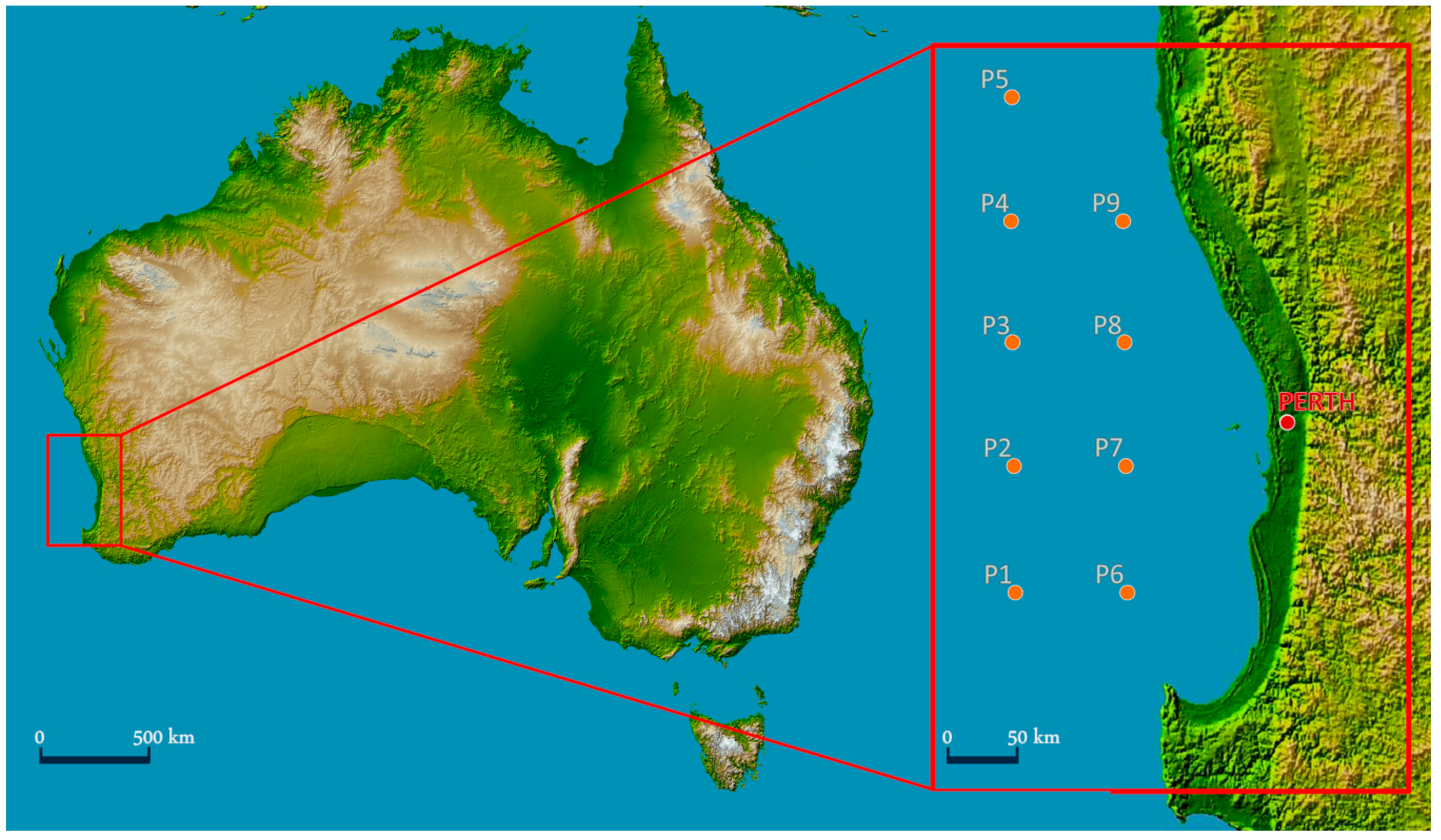
The southwest coast of Australia provides a good case study to illustrate the assessment method. A detailed wave energy assessment is outlined, covering the coastline in one of the most favourable locations in the world for harvesting wave energy. The following summarizes the analysis of offshore and onshore wave power assessment of the Western Australia coasts. The region here considered is the NS oriented coastline, moving from Port Kennedy (45 km south of Perth) to Jurien Bay (about 195 km north of Perth). This coastal area has been chosen for several reasons:

(1)

It represents one of the most energetic regions worldwide [35], although only national-scale wave energy assessments are available [36,37,38,39,40,41,42,43,44,45];

(2)

high seasonal stability level is registered;

(3)

wave climate is characterized by a narrow wave directional sector;

(4)

low tidal excursions, making possible the use of the OBREC technology;

(5)

many harbours, marinas and other coastal defences are present, ensuring high realistic perspectives for OBREC installations (new breakwaters or integrated within existing coastal structures or their upgrades).

Hence, the coastline here analysed can be considered as one of the most favourable regions in the world for harvesting wave energy.

2.1.2. OBREC Technology

Any industrial and/or commercial harbour is a very high energy demanding system: traditional port construction, energy supply and consumption are no longer sustainable. It is necessary to innovate the way we conceive and design the port infrastructure through integration with elements of technological innovation. Within this framework, considerable R&D efforts have been dedicated to evolve from the traditional design concept of coastal structures “dissipating incoming wave energy by wave breaking/absorption” to a new concept of coastal structures “capturing the wave energy”. The breakwater becomes a Wave Energy Converter (WEC). In doing so, unlike all the other WEC installation which are “dedicated” and have an inherently environmental impact (foundations, interaction with wave, currents, sediment transport and vegetation), the WEC functionality of a coastal structure has null relative environmental impact.

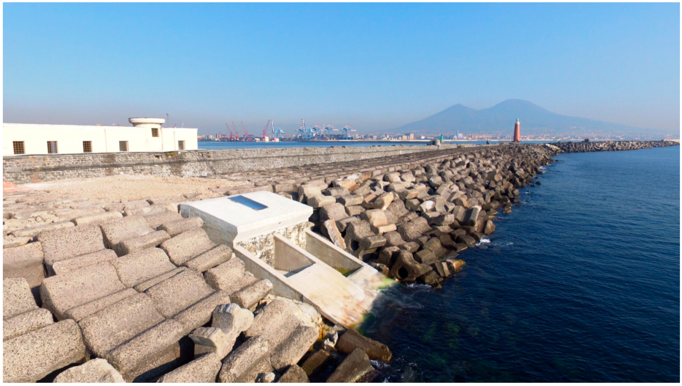
Moving from experience on Sea-wave Slot-cone Generator [4,7,8,46,47], an innovative built integrated device called the OBREC [9] has been developed by the Research team from Second University of Naples. The peculiarities of the OBREC are the easier and less expensive operation and maintenance activities. In fact, it is built as a robust concrete structure with the turbine shaft and the gates controlling the water flow as virtually the only moving part in the mechanical system and the structure is safe even with malfunctioning of these moving parts (Figure 2). Further, thanks to the sharing of the infrastructures and their construction costs (for the function of coastal defence), they tend to be more economically viable than offshore floating WECs, such as Wave Dragon [2] and WaveCat [3].

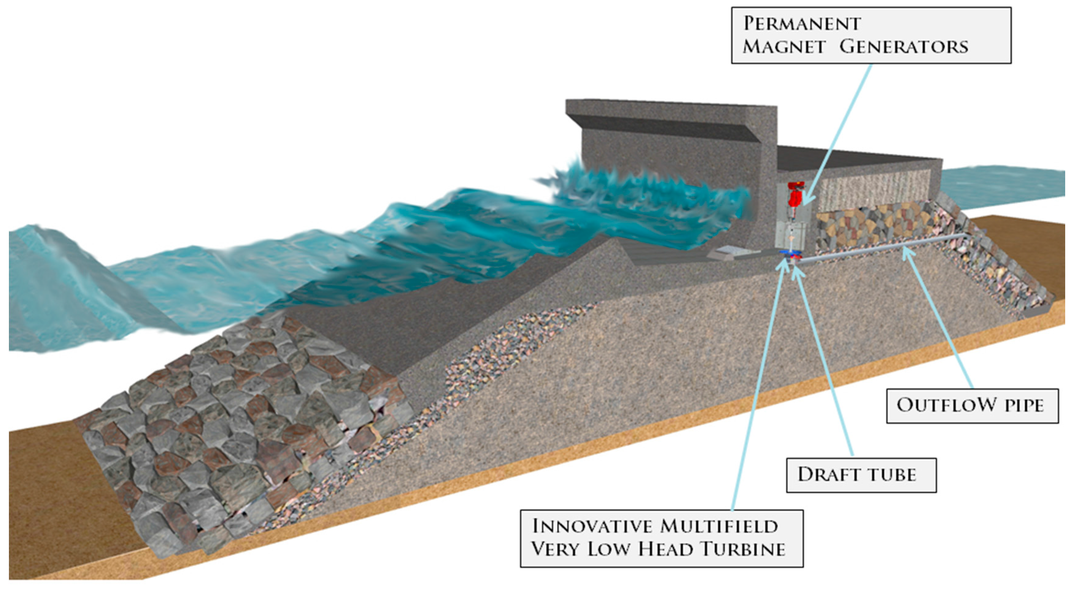
In the machine room, a set of low head turbines convert potential energy (water stored in the reservoirs) into kinetic energy and then into electrical energy by mean generators.

The OBREC prototype at Naples harbour hosts up to five turbines, three of which are already installed. These are low head fixed-Kaplan (propeller) turbines with a permanent magnet generator and a maximum power-point-tracking charge controller. An innovative hybrid “multi-field turbine”, obtained by coupling different kinds of turbine, is currently under development. For upcoming commercial applications, the traditional Archimedean screw turbine could be safely used, which is one of the oldest and most efficient very low head turbines. This screw turbine works on very low head (starting from 1 m or less) and requires relatively less flow rates for generating electricity at a significant level. Its main characteristics are mainly the low initial and maintenance costs and no fine water screening is required. High quality Archimedean screws exceed a design life of 25 years, as experienced worldwide.

2.1.3. Objectives and Approach

The energy production and efficiency of a WEC are always related to the local wave climate. Furthermore, water depths, geotechnical conditions and wave loading on the structure are significant, demanding a site-specific design. The identification of a site-specific design is a very complex process, involving:

• the hydrodynamic performance, such as geometric optimization for energy flux harvesting and reduction of wave loading;
• structural behaviour and fatigue analysis;
• mooring/substructure/structure engineering;
• preliminary environmental constrains;
• inclusion of power absorption;
• electrical cabling and secondary hydro-electrical equipment engineering;
• power take-off, power smoothing and conditioning equipment project;
• control system and strategy;
• transportation feasibility analysis;
• operation and maintenance optimization;
• life cycle assessment and decommissioning.

After a proper site-specific device is designed, the Environmental Impact Assessment analysis must be carried out. This is a very multidisciplinary phase where potential impacts to be considered are [48,49,50]: avoidance of shipping lanes, areas of military importance, marine archaeological sites and other special protection areas:

• landscape and visual impact;
• impacts on marine life and interaction with the marine environment including colonization patterns;
• impact on recreation and other social activities (e.g., industrial fisheries, offshore/onshore platform etc.);
• impact on local marine hydrodynamics;
• sedimentary flow patterns (coastal erosion);
• avoidance of areas of military importance, and marine archaeological sites;
• navigation hazard;
• acoustic noise and bioacoustics;
• electromagnetic impact;
• construction of temporary sites;
• maintains operation impact.

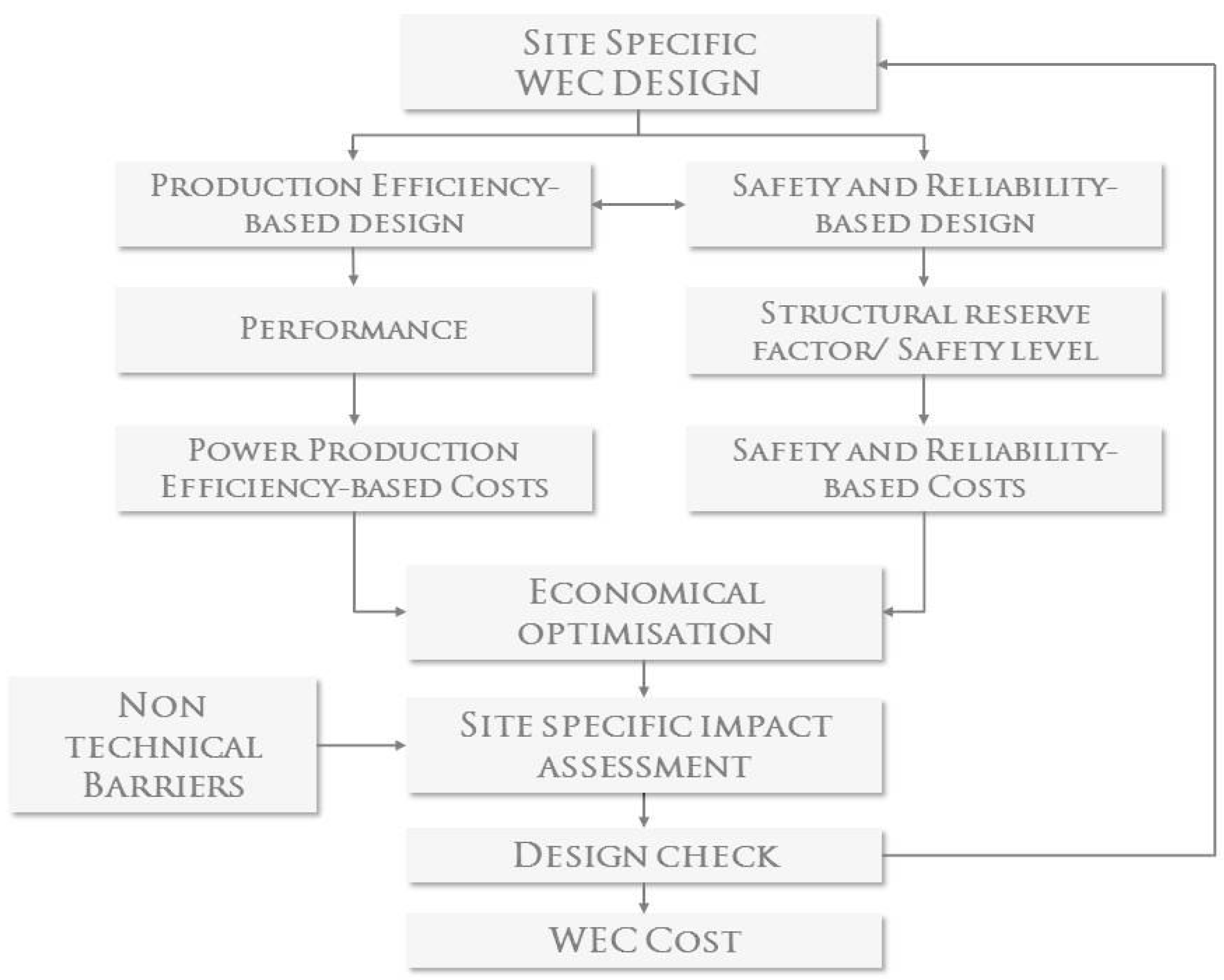
It is well known that the executive WEC design is an outcome of improving a number of intermediate project ideas, satisfying a set of technical and non-technical requirements and subject to constraints. The technical design of a WEC could be synthesized in Figure 3.

The study here presented focuses on the economic feasibility of OBREC installations, disregarding the nature conservation aspects, non-technical barriers and other matters included in the Environmental Impact Assessments related to wave energy conversion.

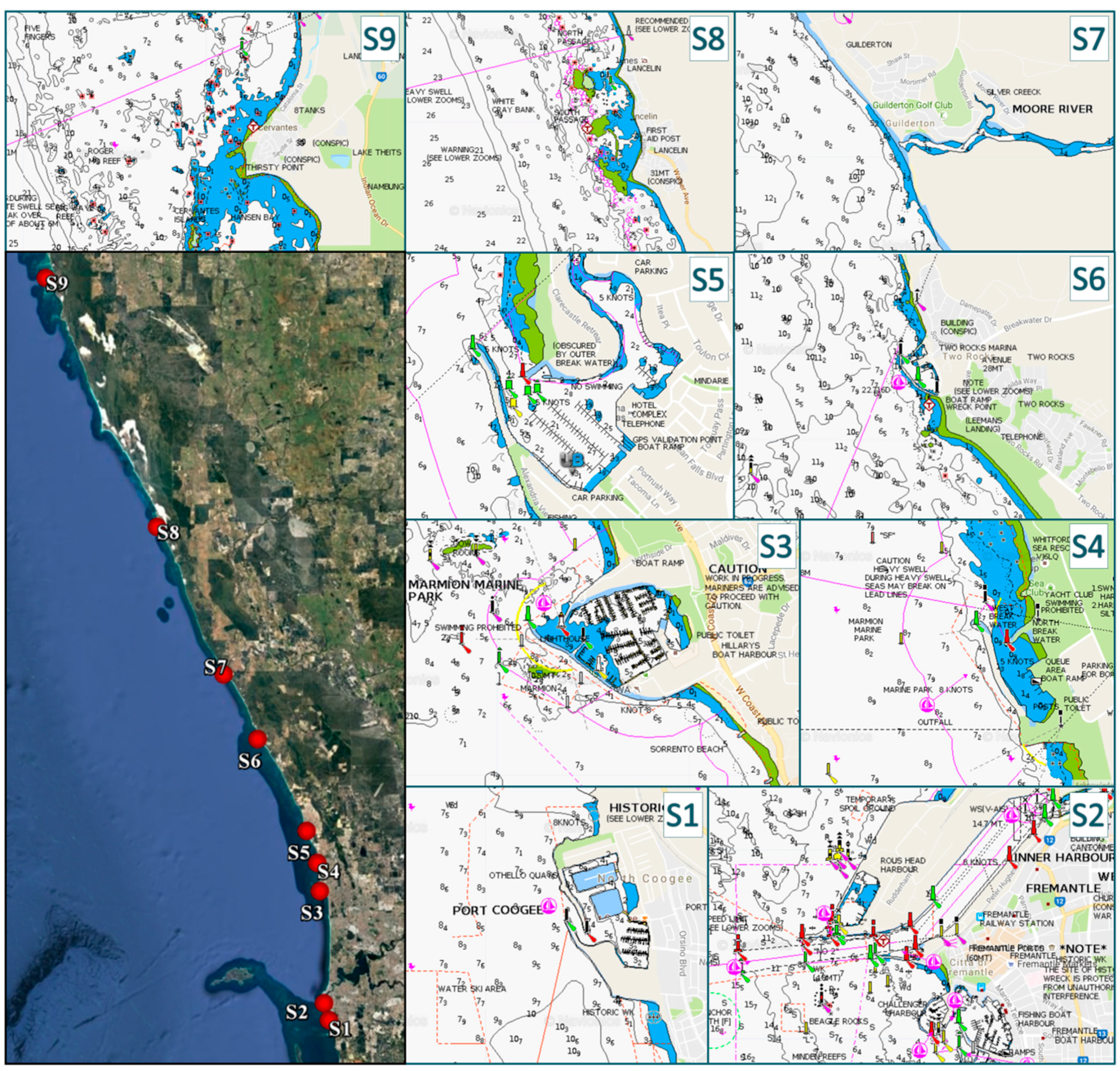
The proposed method works as a comparison analysis under functional, technological and economic constrains between a traditional rubble mound breakwater and the OBREC breakwater. The comparison is applied for 300 m of new main breakwater at each inshore study site described in the following section.

The work hypotheses for the structural design are:

• mean overtopping at the rear of the structures lower than 0.050 m³/s per meter must be ensured;
• foundation design aspects are neglected since geotechnical investigations are not available in the present analysis;
• simple trapezoidal cross-sections (without berm) are considered for the rubble mound substructure;
• armour layer (double layer) consists of sufficiently sized natural stone. In the case of very large stones (>10 tons) resulting from calculus, artificial concrete blocks (e.g., tetrapod) are used.
• Rock slope stability for both types of breakwater; the Van der Meer formulae [51,52,53] has been applied, assuming the fixed parameters reported in

  Table 1. Design parameters used.

  Design Parameters
  slope seaside	1:2
  landward slope	2:3
  initial damage	2
  relative buoyant density	1.65
  notional permeability factor	0.5
  number of waves in the considered sea state	7500

  .

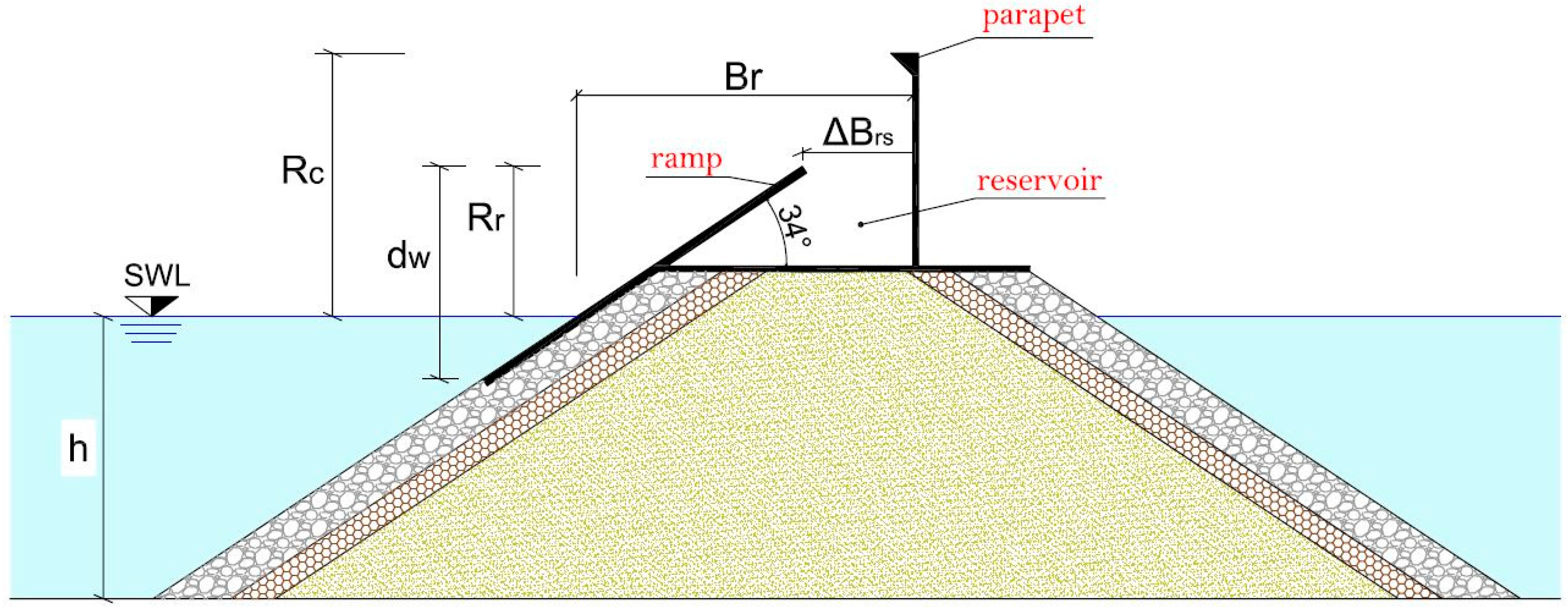
The overtopping at the rear of the structure for traditional breakwater has been estimated with the formula proposed by [54] using parameters proposed by [55]. Once the crown wall crest level is known, Pedersen formulae [56] have been applied in order to estimate wave loadings acting on the structure. For each OBREC, optimal geometry investigated all study sites; the overtopping flow rate at the rear side and the wave loading acting on the device have been estimated using equations proposed by [9]. These formulas have been derived after two complementary model test campaigns were carried out in 2012 and 2014 at the Department of Civil Engineering at the Aalborg University (AAU) in Denmark.

In order to define the turbine strategy, an integrated technical/economic modelling approach has been applied. The purpose is to couple technical and economic parameters that influence the economic profitability of the OBREC technology. Moving from a detailed wave energy resource assessment, an estimation of the energy production of the OBREC at each specific site has been provided. Then, an economic study has been carried out in order to maximize the financial return on investments. The methodology has been applied with the data and procedure described below.

2.2. Wave Propagation

2.2.1. Offshore Wave Energy

The offshore analysis is carried out using the hindcast wave data provided by the European Centre for Medium-Range Weather Forecasts (ECMWF) [57]. The dataset used is a global atmospheric reanalysis from 1979 termed ERA-Interim. The ECMWF internal WAve Model (WAM) covers the Indian Ocean by a base model grid with a resolution of 0.75° × 0.75°. Nine ECMWF grid points (P1–P9), covering a latitude from 30°S to 33°S with a longitude ranging between 114°E to 114.75°E, have been selected to characterize the offshore energetic patterns (Figure 4). Geographical information of ECMWF grid points are reported in

Table 2. Geographical information of ECMWF grid points P1–P9.

Point	Depth (m)	Lat	Lon
P1	1939	33°00′0.00″S	114°00′0.00″E
P2	4289	32°15′0.00″S	114°00′0.00″E
P3	4738	31°30′0.00″S	114°00′0.00″E
P4	4549	30°45′0.00″S	114°00′0.00″E
P5	1652	30°00′0.00″S	114°00′0.00″E
P6	513	33°00′0.00″S	114°45′0.00″E
P7	572	32°15′0.00″S	114°45′0.00″E
P8	559	31°30′0.00″S	114°45′0.00″E
P9	369	30°45′0.00″S	114°45′0.00″E

. The WAM provides 6-h values of significant wave height (H_s), mean wave period (T_m) and mean wave direction (θ_m). From a 6-h triple (H_s, T_m, θ_m) dataset, ranging from January 2005 to December 2014, the average wave power has been computed for P1–P9. Operatively, the approximate deep water expression for the wave energy flux, P, has been applied

$$P=\frac{\mathsf{\rho }\times g^2\times H_{mo}^2\times T_e}{64\times \mathsf{\pi }}$$

(1)

where $\mathsf{\rho }$ is the sea water density, g is the gravity acceleration, $H_{mo}$ is the wave height computed on the zero-order moment of spectral function and T_e is the wave energy period. Following a conservative approach, according to [58], the energy period has been assumed as 1.14 T_m.

2.2.2. Nearshore Wave Energy

The nearshore wave energy patterns have been determined applying the MIKE 21 SW model for wave propagation in nearshore regions. The model used is MIKE 21 SW, developed by DHI (Danish Hydraulic Institute) Water and Environment. The basic equations in the model are derived from the conservation equation for the spectral wave action density, based on the approach proposed by the authors of [59]. The computational domain was discretized using an unstructured grid with meshes based on linear triangular elements (Figure 5). The domain boundary was chosen to coincide with a polyline passing through five ECMWF points: P1, P2, P3, P4 and P5. The seabed was performed by interpolating at the grid nodes the information provided by the General Bathymetric Chart of the Oceans (GEBCO) database [60] (Figure 5). The grid resolution has been assumed to be variable linearly between 1000 m to 150 m for the depth in the range 500 m to 100 m. Constant values of 150 m and 1000 m of the grid resolution have been assumed respectively for water depth shallower than 100 m and deeper than 500 m respectively. Although the latest release of the 30 arc-second global bathymetric grid has been used, the GEBCO database could not be of good attainability in very shallow water. Hence, the offshore dataset of waves has been propagated to depths of 20 m, as representative of the nearshore wave power. The 20 m-isobath seems very significant considering that several moored and founded WECs installations could be installed at that depth [61,62].

2.2.3. Inshore Wave Energy

In order to envisage potential locations for the OBREC in correspondence of urban coastal defences, commercial harbours and marinas along the coastline, nine study sites (S1–S9) have been investigated in detail (Figure 6). In

Table 3. Geographical l information of nearshore study sites.

Point	Locality	Lat	Lon	Depth (m)
S1	Port Coogee	32°6′8.67″S	115°45′2.64″E	9
S2	Fremantle	32°3′56.95″S	115°44′19.95″E	7
S3	Hillarys boat harbour	31°49′23.58″S	115°43′53.06″E	7.5
S4	Ocean reef boat harbour	31°45′45.27″S	115°43′32.49″E	7.5
S5	Mindarie	31°41′35.79′′ S	115°41′58.46″E	7.5
S6	Two rocks	31°29′43.00″S	115°34′38.66″E	7.5
S7	Guilderton	31°21′17.34″S	115°29′35.26″E	7.5
S8	Lancelin	31°2′2.61″S	115°19′42.57″E	7.5
S9	Cervantes	30°29′21.02″S	115°3′9.53″E	7

, the approximate water depth and other geographical information for each specific site are reported. Therefore, according to the previous nearshore wave propagation analysis, the wave characteristics at the points S1–S9 have been derived through a process of wave transformation mostly performed manually. This study takes into account refraction, shoaling and wave-breaking moving from wave patterns analysed on a 20 m-isobath. For S1 and S2, a directional analysis has also been carried out, considering that waves from directions below 235° and 220° respectively are hindered, due to the presence of Garden Island. The energy diffraction around Carnac Island (at a distance of about 10 km) is also considered, implying about a 30% loss of the energy coming from the angular sector covered. The general approach in this shallow water analysis can be considered a conservative estimation of wave energy.

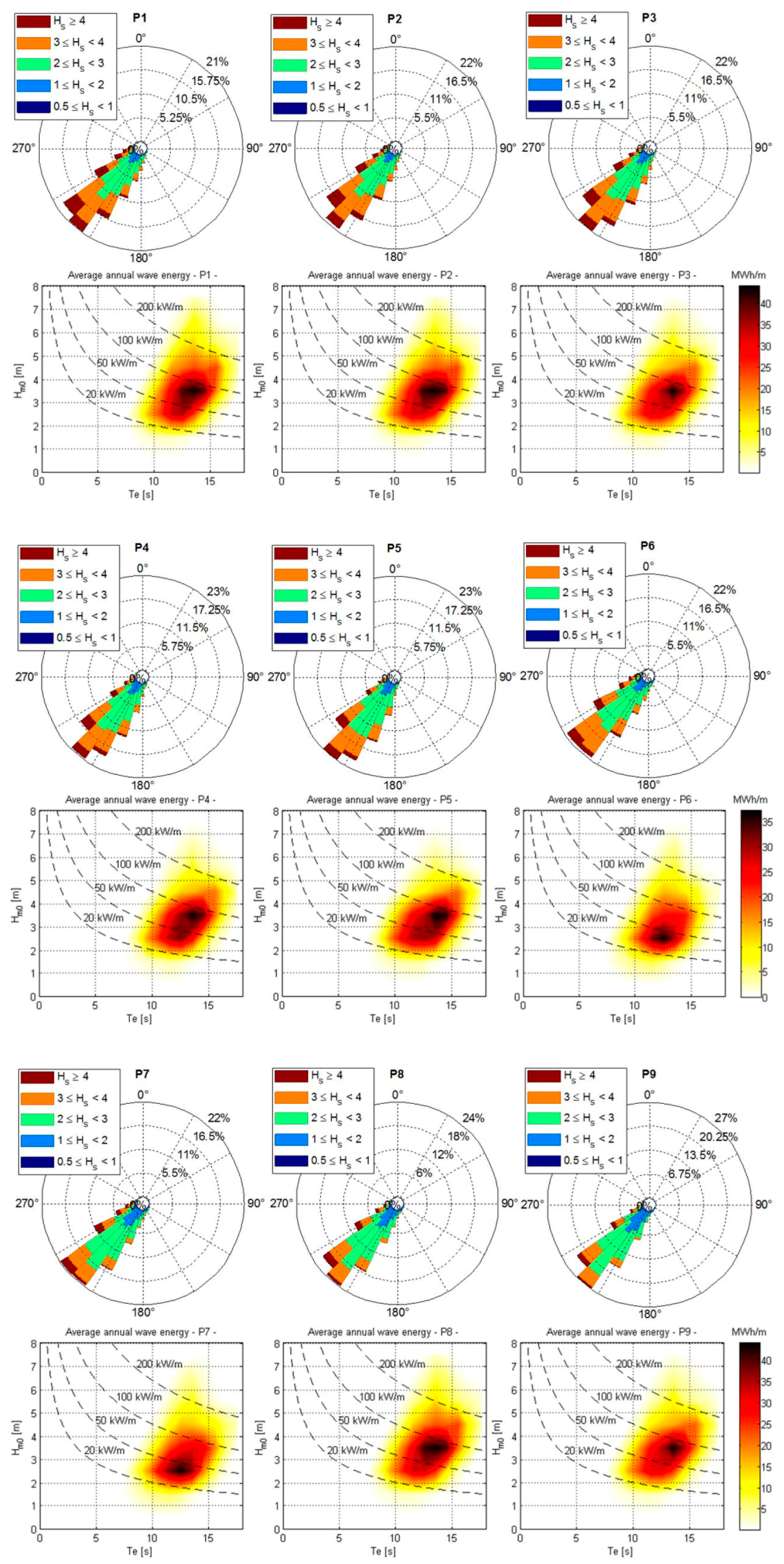
2.3. Resource Analysis

The expected energy production of a WEC can be estimated crossing the power matrix with the incident wave conditions (e.g., [20,27]. The OBREC prototype at Naples harbour (Italy), in operation since January 2016, represents the world’s first overtopping WEC totally integrated into an existing breakwater. As the monitoring has just begun, no definitive power matrix is available. For that reason, conservative values for power efficiency parameters are adopted in the present study. Considering the multiple interdependencies between the parameters involved, the only practical approach to solve the complexity of the optimisation task is represented by a software simulation of the system behaviour combined with a systematic parameter variation. A specially designed numerical model (OBRECsim) has been used to simulate energy production. The aim of the simulation is to determine the optimal geometry of the device and turbine strategy for which the energy production is maximized. The input parameters are:

• wave characteristic of sea states;
• tentative geometry of the device;
• tentative turbine configuration.

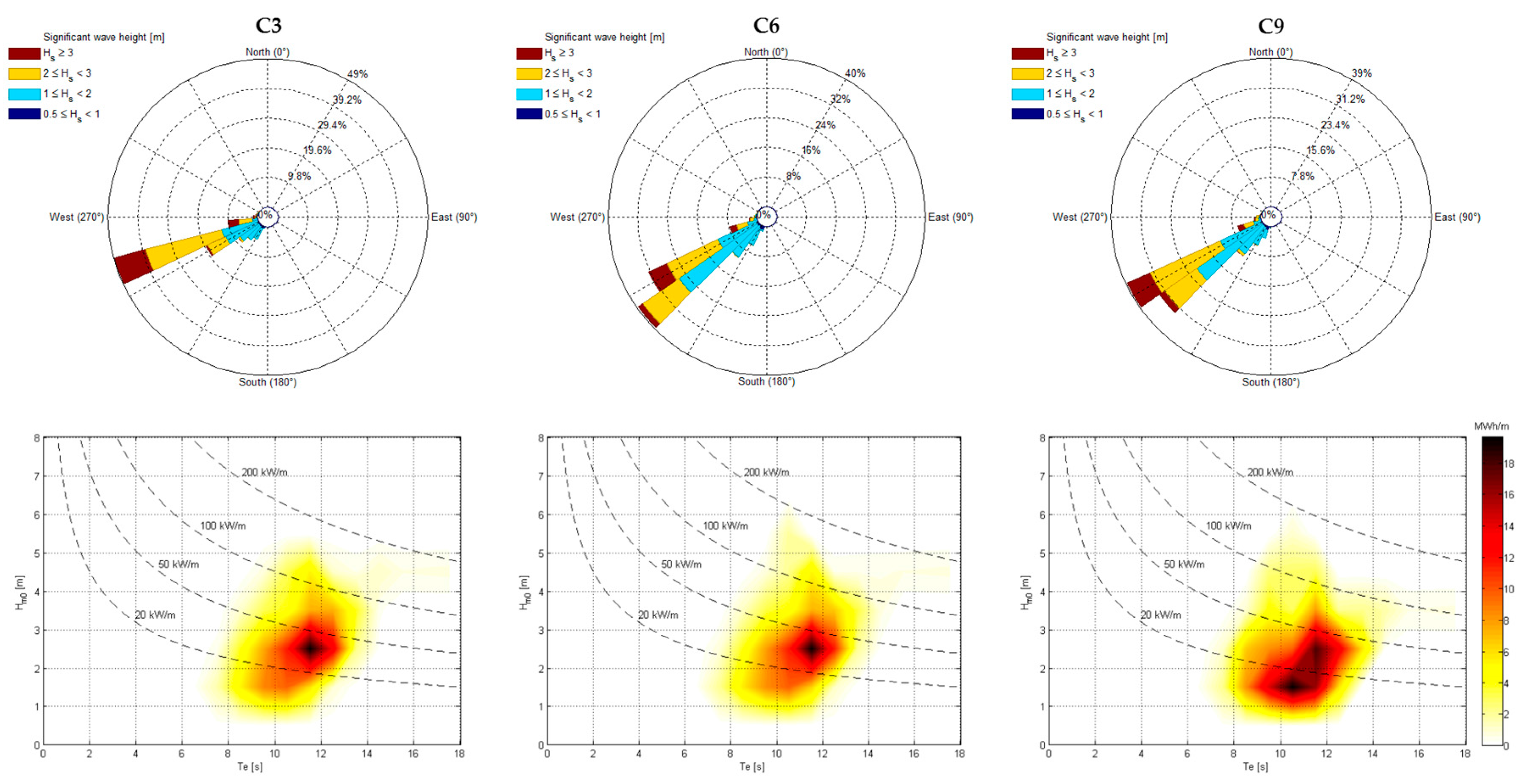
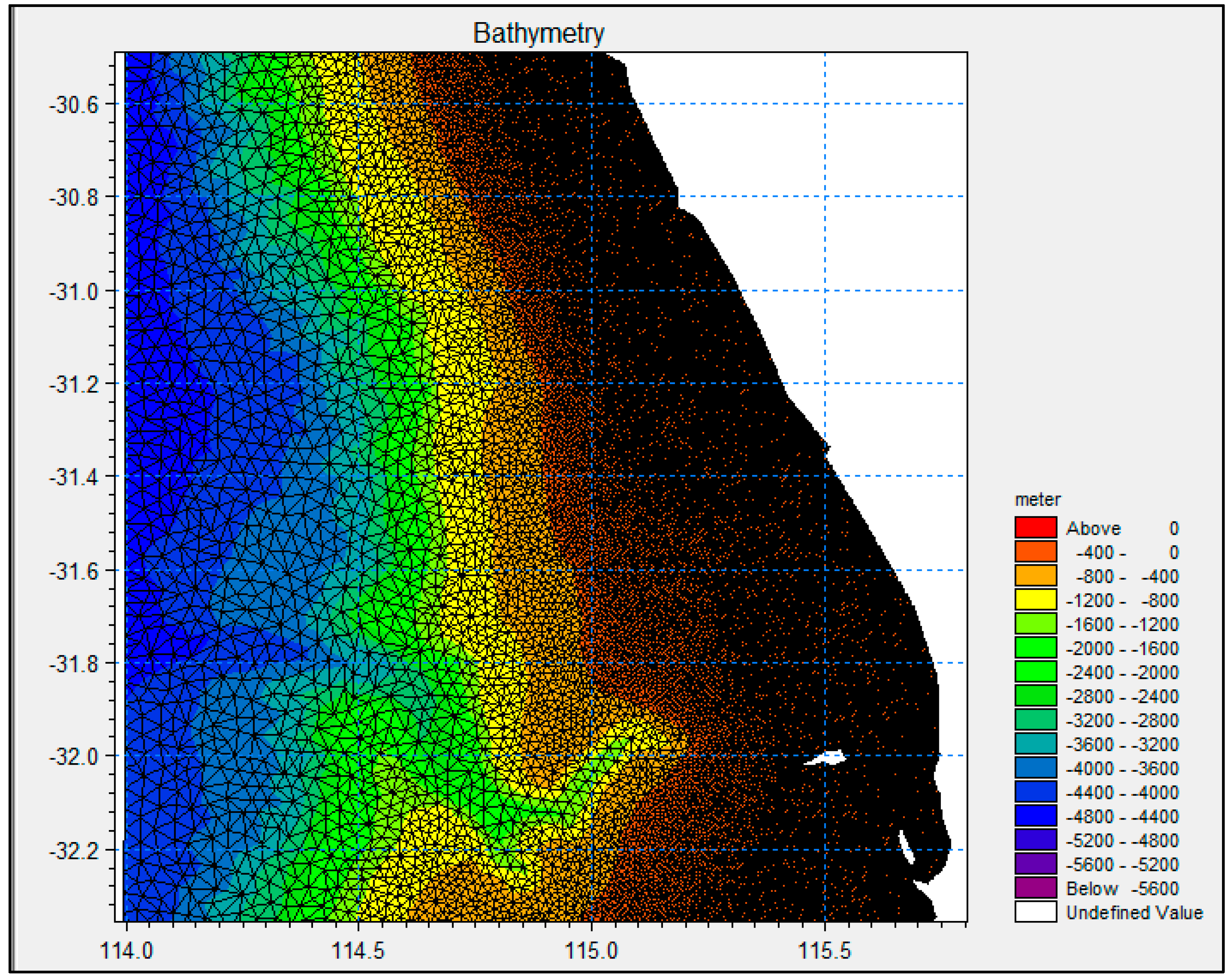
Operatively, the waves from 10 year averaged 6 h triple dataset for S1–S9 were grouped by classes of H_s–T_p−θ_m. The code simulates a time series of the mean water flow into the reservoir. The latter is found using the overtopping formula provided by [9]. The numerical model is based on the continuity equation:

Qin = Qreservoir + Qrear + Qoverflow

(2)

where Q_reservoir is the flow through turbines, Q_rear is the overtopping flow rate at the rear side of the structure and Q_overflow is the reflected flow outgoing when the reservoir is saturated. In order to estimate electricity production, four levels of efficiency are taken into account:

-

efficiency of the ramp, i.e., rate of total incident power overtopping the crests;

-

efficiency of the reservoir, in terms of potential energy stored or lost for overflow in the reservoirs;

-

turbines efficiency, as potential energy transformed into kinetic energy by turbines and related to start/stop penalties;

-

electromechanical efficiency, as power take-off and generator efficiency and inverter losses.

In order to estimate the energy production, the efficiency curve of traditional turbines has been used in the present analysis. For each study site, different number and types of turbines are taken into account for optimisation analysis.

2.4. Economic Analysis

The so-called payback period method has been selected in this research as the economic analysis technique. This payback period is defined as the time required to completely recover the initial investment. It can be considered a significant determinant in a capital budgeting decision framework, as longer payback periods are typically not desirable for investment positions. Unlike other methods of capital budgeting, the method ignores the benefits that occur after the investment is repaid, while it could be effective in measuring investment risk. The formula to calculate payback period (PBP) expressed in years, is:

$$PBP=\frac{CAPEX}{C_i-C_o}$$

(3)

where:

-

CAPEX (Capital expenditures) represents the initial investment assumed to be paid at time t = 0;

-

C_i is the cash inflow, i.e., the annual revenue (AR) generated by incentive on renewable energy and/or electricity sales;

-

C_o is the annual cash outflow, due to operational and maintenance costs for the power system of OBREC (OPEX).

Due to the complex analysis of the OBREC financial performance, a second indicator is also chosen. This is the Net Present Value (NPV), by which the profitability of a project could be easily quantified along its lifetime (LT). It is expressed as:

$$NPV=-CAPEX+{{\displaystyle \sum }}_{t=1}^{LT}\frac{AR-OPEX}{{\left(1+r\right)}^t}$$

(4)

CAPEX are calculated as:

$$CAPEX=CAPE{X}_{EM}+CAPE{X}_{MW,trad}-CAPE{X}_{MW,OBREC}$$

(5)

where CAPEX_EM is the cost of electro-mechanical equipment, which is added to extra cost (or cost saving) related to Maritime Works necessary to build the OBREC breakwater instead of a traditional breakwater (CAPEX_MW,OBREC and CAPEX_MW,trad respectively) with the same overall safety performance.

Cable costs are mainly estimated on the basis of the number of turbines or modules’ length, assuming that the point of connection of the OBREC breakwater is electrified. The value of the discount rate, r, largely affects the financial analysis. The indicative discount range for fixed WEC was 10%–14% [63,64,65]. For comparison, traditional hydroelectric power generation had the discount rate 6%–9% [65]. As known, the uncertainty about the specific value of r increases with risk perception, often leading to internal inconsistencies in the mechanism used to estimate it. In this vein, the OBREC shows a less relative immaturity compared to other WEC technologies, being a fixed breakwater where waves operate on a quasi-traditional hydroelectric power system. For this reason, a nominal annual discount rate of 9% is fixed. According to the approach used by [20], considering expected inflation of 1.3% [66], a resulting real interest rate of 7.7% is assumed.

Policy mechanisms (e.g., feed-in-tariff) designed to accelerate investment in the wave energy sector in Western Australia are not yet defined, as is the case in several countries. For this reason, a probable socioeconomic scenario has been here defined, based on the feed-in tariff scheme applied in Western Australia to encourage the expansion of a residential solar energy system [67]. Hence, the following assumptions have been made:

(1)

a net feed-in-tariff of 40 cents per Kilowatt-hour over the next ten years, complementary to 8.4 cents currently paid under the Renewable Energy Buyback Scheme within the South West Interconnected System;

(2)

the energy produced is not consumed by the producer (the Port Authority) during the first ten years, meaning a total of 48.4 cents for each unit of electricity exported to the grid;

(3)

starting from the eleventh year, an average quote of 43% of electricity produced is directly consumed by the producer (reducing or helping meet peak demand);

(4)

considering energy saving due to the self-production (with a mean electricity cost of 35.35 AUD/KWh) and the buyback excess electricity rate of 8.4094c per kWh (on 57% of total production) the effective value of electricity produced after this can be estimated as 20 cents per KWh.

For the calculation of CAPEX_EM and OPEX, two options (Option 1 and 2) have been applied (see

Table 4. Proposed option on turbine architecture for the study.

Characteristic/Option	Option 1	Option2
Turbine architecture	Propeller	Screw/low head Kaplan turbines
Turbine strategy	Several (>200) pico turbines	Some (5–13) micro/mini turbines
Turbine lifetime (years)	6	24
Yearly OPEX costs (per cent of initial equipment cost)	0.055	A 0.2% annual raise level, from 2.8% to 7.4%

). In Option 1, power production optimization was made using a large number of very economic propeller turbines. These turbines dominate the low head sector of the hydroelectric market. The model here used is one of the cheapest pico-turbines (ex-works price is AUD 1177.72 [68]), with nominal power of 1.5 kW at 3 m head and a flow rate of 0.045 m³/s. Its ex-works price is AUD 1177.72 [68] and Based on the field experience made on the OBREC prototype, to that price the costs for an inox runner (AUD 400.00), plastic shaft (AUD 260.00), filter (AUD 140.00) and shipping (AUD 430.00) should be added. The cost of civil works that need to be completed to allow the scheme to run, broken down into intake, turbine mounting, outflow requirements and powerhouse is estimated at AUD 865. Therefore, the expected cost of the whole hydro-electromechanical system was fixed at AUD 2185.00 per kW.

The yearly operational and maintenance costs (OPEX) for pico-propellers are estimated as 5.5% of the initial cost, based on a conservative approach and experience gained from the OBREC prototype. A conservative equipment life of only 6 years has been selected. Hence, a complete replacement of pico turbines (and its inox runners), at least four times over a range of system lifetimes (24 years), is taken into account.

In Option 2, larger turbines are considered. In the first instance, the selected turbine architecture was the screw turbine, which works on low head and requires less flow rates that can be used for generating electricity at micro level. However, when the optimization procedure leads to flow rates greater than 5–6 mc/s, due to size problems (i.e., very large machine rooms are required, clearly in opposition with the confined space behind the crown wall), very low head (VLH) Kaplan turbines were used. Based on literature data and personal communication of a quote for the OBREC prototype, the costs of electro-mechanical equipment (including rotor, power train, generator and other equipment, cable costs, installation costs and grid connection costs) and related civil works (CAPEX_EM) can be estimated using the following expressions:

For screw turbine

$$CAPE{X}_{EM}=3550P+75,600[\mathrm{A}\$]$$

(6)

For Kaplan turbine

$$CAPE{X}_{EM}=4000P+105,000[\mathrm{A}\$]$$

(7)

where P is the rated power (KW). Both equations have been calibrated on turbine size range and other technical specifications for OBREC operability (e.g., seawater corrosion inhibitors or cathodic protection, special hydraulic works, etc.). A 24 year technical and economic lifetime was assumed, although it is thought that the quality equipment used could reasonably last 25–27 years. The OPEX cost for screw and VLH Kaplan turbines in available projects suggested values ranging between 1.5% and 7% of the total project initial cost. In this study, an initial value of 2.8% with an annual raise level of 0.2% (i.e., a value of 7.4% at the 24th year of operative life) is assumed.

3. Results

3.1. Wave Energy Resource

3.1.1. Offshore Wave Energy

In

Table 5. Main wave climate parameters (based on 10 year average) at ECMWF grid points.

Point	Hs,mean	Hs,max	Hs,min	σH	Tm,mean	Tm,max	σT	Te,mean	θm
	(m)	(m)	(m)	(m)	(s)	(s)	(s)	(s)	(°)
P1	3	8.82	0.95	0.9	10.63	16.77	2.78	12.12	218.12
P2	2.98	8.68	1.01	0.85	10.63	16.78	2.85	12.12	216.3
P3	2.91	8.44	1.02	0.78	10.64	16.76	2.87	12.13	215.61
P4	2.83	8.01	1.02	0.71	10.64	16.85	2.87	12.13	215.06
P5	2.79	7.54	1.01	0.66	10.62	16.85	2.92	12.11	214.12
P6	2.58	7.58	0.83	0.7	10.39	16.55	2.65	11.84	221.81
P7	2.62	7.92	0.9	0.7	10.46	16.72	2.77	11.92	219.77
P8	2.59	7.79	0.88	0.66	10.58	16.79	2.76	12.06	219.32
P9	2.46	7.3	0.78	0.59	10.68	16.79	2.7	12.17	220.55
Mean	2.75	8.01	0.93	0.73	10.59	16.76	2.80	12.07	217.85
σ	0.18	0.53	0.09	0.1	0.09	0.09	0.09	0.11	2.71

and

Table 6. Monthly and yearly wave power (based on 10 year average) at ECMWF grid points.

Point	Average Monthly Power (kW/m)												Yearly Average
	January	February	March	April	May	June	July	August	September	October	November	December
P1	41.8	37.9	45.6	57.0	66.4	77.0	89.7	87.0	97.1	63.3	43.4	37.4	62.0
P2	42.1	37.8	45.3	55.9	65.2	74.9	87.6	84.7	94.5	62.4	42.9	37.4	60.9
P3	44.2	36.5	43.4	53.0	62.0	70.6	82.8	79.9	89.1	59.6	41.2	36.1	58.2
P4	39.6	34.8	41.1	49.8	58.4	66.1	77.7	74.9	83.4	56.6	39.3	34.6	54.7
P5	38.9	33.8	39.7	47.8	56.2	63.2	74.1	71.6	79.6	54.8	38.2	33.8	52.6
P6	31.3	27.7	33.4	41.6	49.8	58.0	68.2	65.7	73.5	47.9	33.0	27.8	46.5
P7	33.9	27.6	33.1	41.0	49.2	56.6	66.8	64.4	71.9	47.7	32.9	27.8	46.5
P8	30.8	24.9	30.0	37.3	45.0	51.2	60.7	58.7	65.5	44.0	30.3	25.4	46.1
P9	39.3	32.5	38.3	46.4	54.8	61.7	72.4	69.9	77.8	53.5	37.2	32.8	42.0
Mean	38.0	32.6	38.9	47.8	56.3	64.4	75.5	73.0	81.4	54.4	37.6	32.6	52.7

, the main parameters of wave climate and the assessment of the monthly and yearly mean wave power have been summarised at ECMWF grid points, P1–P9. Results are based on 10 year average. The annual wave power was found to range between 42 kW/m (P9) and 62 kW/m (P1), the bulk of which is provided by south-easterly waves. A tentative contour map of wave power isolines, spacing 5 kW/m, is reported in Figure 7. The results are graphically represented with polar diagrams assembled in Figure 8. Moreover, characterization of the yearly average wave energy in terms of significant wave height (Hm0) and energy period (Te) is also reported. The colour scale represents annual energy per meter of wave front (in MWh/m). The numbers within the graphs indicate the occurrence of sea states and the isolines refer to wave power.

3.1.2. Nearshore Wave Energy

To enable an immediate visual identification of the energy flux variation, also in the perspective to better visualize potential locations for offshore WEC farms, an energy flux density contour on 20 m-isobaths was computed. The relative colour band is shown along the analysed coastline in Figure 9. Ten control points (C1–C10) are also indicated.

Table 7. Geographical information and main wave climate parameters (based on 10 year average) at points C1–C10.

Point	Lat	Lon	Depth (m)	Hs,mean	Hs,max	σH	Tm,mean	σT	Te,mean	θm	Power,mean
				(m)	(m)	(m)	(s)	(s)	(s)	(°)	(KW/m)
C1	32°23′60.00″S	115°35′60.00″E	−19.99	1.68	4.73	0.36	9.84	2.05	10.2	247.46	17.65
C2	32°12′0.00″S	115°35′24.00″E	−19.66	1.76	5.01	0.42	9.86	2.01	10.22	240.94	18.35
C3	32°1′12.00″S	115°26′16.80″E	−24.22	2.24	6.08	0.72	9.86	2.03	10.21	244.03	30.07
C4	31°48′0.00″S	115°38′24.00″E	−20.58	1.64	4.79	0.5	9.87	1.99	10.22	245.38	16.87
C5	31°36′0.00″S	115°34′48.00″E	−22.05	1.97	4.97	0.54	9.88	1.95	10.23	234.83	20.89
C6	31°23′60.00″S	115°27′0.00″E	−21.16	1.99	5.13	0.5	9.87	1.99	10.22	233.12	22.81
C7	31°12′0.00″S	115°17′60.00″E	−21.75	2.01	5.24	0.59	9.88	1.95	10.23	234.85	23.45
C8	31°0′0.00″S	115°15′36.00″E	−20.78	2.02	4.88	0.46	9.88	1.96	10.23	235.81	24.02
C9	30°47′60.00″S	115°8′24.00″E	−19.69	2.09	5.14	0.5	9.87	1.96	10.23	232.76	24.51
C10	30°36′0.00″S	115°2′24.00″E	−20.94	2.12	5.32	0.49	9.87	1.96	10.23	228.43	25.43

presents geographic information, main wave climate parameters and the related wave power potential for these points. To identify the influence of each sea state, diagrams on yearly average source have been assembled in Figure 10 for C3, C6 and C9, mainly as representative. In each class, the significant wave height and energy period values are spaced, respectively, at 1 m and 2 s. The analysis highlighted the presence of a “hot spot” in correspondence of Eagle Bay in Rottnest Island (Point C3), with an annual mean wave power of 30 kW/m. Here, the loss of power as the waves travel towards the shoreline is partially compensated by natural energy concentration due to a relatively steep bathymetry. In particular, a very narrow wave sector could be recognized, essentially attributed to the presence of Perth canyon. Indeed, this is an area where wave energy developers are currently focussing efforts (e.g., Carnegie Wave Energy Ltd., Fremantle, WA, Australia, Perth Wave Energy Project [69]).

3.1.3. Wave Climate at Study Site

Main wave climate parameters, average wave power and yearly energy per meter of wave front at each study site are reported in

Table 8. Main wave climate parameters at each study site.

Point	Hs (m)	σ	Tm,mean (s)	θmean (°)	Te,mean (s)	HD (m)	Average Power (kW/m)	Yearly Energy (MWh/m)
S1	1.85	0.57	7.89	242.49	9.70	5.87	15.25	133.44
S2	1.77	0.55	7.89	244.31	9.70	5.93	15.78	138.08
S3	1.51	0.50	7.90	245.48	9.70	5.20	12.89	112.79
S4	1.57	0.51	7.90	243.35	9.71	5.02	13.80	120.76
S5	1.67	0.52	7.90	240.16	9.71	5.25	15.71	137.47
S6	1.83	0.52	7.90	233.97	9.71	5.73	16.52	144.56
S7	1.85	0.50	7.90	233.10	9.70	5.43	17.31	151.47
S8	1.86	0.48	7.90	234.46	9.71	5.35	17.62	154.18
S9	1.91	0.49	7.90	232.12	9.71	5.54	17.79	155.67
Mean	1.76	0.52	7.90	238.82	9.71	5.48	15.85	138.71

. Significant wave heights range between 1.51 and 1.91 m, while very similar mean wave period and energy period were found (on average 7.90 s and 9.71 s respectively). The annual power was found to range between 12.89 and 17.79 kW/m. About 60% of total power is related to waves between 9 and 12 s. About 55% of the total resource is provided by waves with significant heights between 1 and 2 m, and about 30% by significant wave heights between 2 and 3 m. Very similar maximum wave period was found for each site (T_m,max = 13 s).

A noteworthy issue is the wave climate design condition. In fact, wave conditions for a return period of 50 years should be considered in the analysis; however, the design wave height is deliberately underestimated for two key questions:

(1)

in a preliminary study on the economic assessment of the OBREC, it was recognized that the higher the design wave height, the greater the cost saving by using the OBREC breakwater instead of traditional coastal protection; therefore, for a conservative economic analysis, a lower value of design wave height and related wave period should be assumed;

(2)

the tendency to underrate significant wave height values during storm conditions performed by the ECMWF dataset is evidenced in several studies [58,62,70,71,72,73]. This behaviour turns directly into not-reliable long-term return level estimates for extreme wave analysis, leading to a weak description of wave climate [74,75].

Therefore, based on long-term estimates of extreme significant wave heights provided by the ECMWF dataset, the design wave heights, H_D, for a return period of 25 years, have been used (Table 8). For each site, the design period, T_D = T_m,max has been assumed.

3.1.4. Wave Hindcast and Wave Model Validation

The detailed validation of the ECMWF hindcast model and MIKE 21 SW are out of the scope of the present paper. However, it is really important to ensure that accuracy in the calculation of the energy flux can be considerate acceptable from an engineering point of view. The ECMWF model uses the current best description of the model physics. Therefore, the hindcasts from it (ERA-Interim) can be considered reliable and generally slightly conservative for wave energy assessing. The underestimate of ECMWF data was previously highlighted within the WW-Medatlas projects [70] and through intercomparison with NCEP (National Centers for Environmental Prediction) Climate Forecast System Reanalysis [72]. Moreover, comparison with wave buoy data worldwide shows lowest values of energy in the ECMWF points, especially in the highest power class (e.g., [58,62,71,73,74,75]. These differences can be attributed mainly to the dissimilar measurement condition. The smaller sampling frequency for the hindcast data involves peak attenuation, acting as a band-pass filter and smoothing the signal. Furthermore, it should be noted, as in the typical spectrum of this meteorological model, that the energy drops rather abruptly to 0 at about 200 km; a dimension comparable to the model grid resolution. Hence, the use of the ERA-Interim dataset could be considered adequate for slightly conservative wave power potential and studying the long-term variation in wave height [74] but, at the same time, should be examined carefully during detailed resource assessments or for arriving at the design wave condition. The MIKE 21 SW model has been validated by comparison with data from buoys and satellites by several authors [58,62,76,77,78,79]. This model was previously applied along the Victorian coast by the Sustainable Energy Authority Victoria, and comparison between computed values and waverider buoy records of H_s was carried out [80]. These estimates are reported to adequately simulate direct measurements at Cape Sorell and Portland, while slightly overestimating H_s at Point Lonsdale. Historical Australian wave buoys data are not collected in a unique data warehouse, compromising an easy consultation. Only since 2004, an open-access Australian Wave Energy Atlas (AWavEA) has been under development, and it is scheduled for completion in 2017 [81]. For this reason, verification has been carried out in the form of a comparative analysis of data provided in the scientific literature.

Authors of [44] report a revised assessment of Australia’s national wave energy resource, validated by in situ wave buoy and satellite altimeter observations. The model resolution of the computational grid moves from 44 to 7 km landward direction. For the area covered by ECMWF points P1–P9 (with bathymetry from 4800 m to 370 m), a mean wave energy flux ranging between 40 and 65 kW/m was found, according to results previously shown in Figure 7. Similar results were observed by [39]. Authors reporting an analysis on wave-rider buoy data sets (1998–2006) for Cape Naturaliste, found an average significant wave height of 2.50 m, a mean peak period of 13.1 s and an average energy flux of 39 kW/m at a water depth of 25 m. These values are coherently observed for ECMWF point P6, about 70 km north-west of Cape Naturaliste, where the average significant wave height of 2.58 m, a mean peak period of 13.5 s (as 1.14 T_e in Table 6) and an average energy flux of 45 kW/m at a water depth of 500 m have been computed. In [38], a mean significant wave height of 2.21 m and a mean wave power of 28.56 kW/m for the most energetic site in about 50 m depth off Western Australia were evaluated. These results seem consistent with the energy pattern found at about 20 m water depth in this study (see Table 7). Moreover, wave buoy data collected under a 2.5-year period (1994–1996) lead to an annual mean wave power estimation of 48 kW/m in a 48 m water depth south-west of Rottnest Island [82]. Considering the short period and the highest peak values affecting the estimate by buoy measurements, these results give confidence in the 30 kW/m found in this study at 20 m depth.

3.2. Site-Specific OBREC Design

3.2.1. Structural Design

The design of the OBREC is a complex matter and had to be conducted as a whole, i.e., each parameter involved is able to have a significant effect. For example, the crest freeboard, R_r, which defines the maximum water head on the turbines, strongly affects the overtopping at the rear side and wave loading on the structure.

Three key aspects in the OBREC design could be synthetized:

• hydraulic protection;
• structural safety;
• hydraulic efficiency of the sloping front-reservoir.

The depth inside the reservoir, h_r in Figure 11, has been chosen as 0.5 m, in order to ensure a significant level of minimum water head acting on turbines (e.g., the reservoir bottom is 1.4 m from swl for R_c(S3) = 1.9 m).

A cross-section of the geometric parameters at each study site, as resulting from computational analysis, are reported in

Table 9. OBREC cross-section geometric parameters at each study site.

Site	Rr	Rc	ΔBr	Br	ΔRc	dw	qrear	CAPEXMW
	(m)	(m)	(m)	(m)	(m)	(m)	(mc/s)	(AUD/m)
S1	2.4	7.2	7.7	11.2	4.8	3.9	0.046	88528.3
S2	2.3	6.8	6.9	10.3	4.5	3.8	0.048	71906.9
S3	1.9	6.4	6.0	9.0	4.4	3.5	0.047	50591.1
S4	2.0	6.3	6.3	9.4	4.2	3.6	0.046	47477.0
S5	2.1	6.6	6.6	9.9	4.4	3.7	0.044	51167.9
S6	2.4	7.1	7.2	10.8	4.7	3.9	0.049	76724.0
S7	2.4	6.8	7.2	10.8	4.4	3.9	0.050	72508.4
S8	2.5	6.8	7.5	11.2	4.3	4.0	0.049	73706.4
S9	2.5	7.0	7.5	11.2	4.5	4.0	0.047	74336.9

, where:

• R_r is the crest freeboard of the front ramp;
• R_c is crest freeboard of the crown wall;
• B_r is the emerged structure width in correspondence of still water level;
• ΔB_r is the reservoir width;
• d_w represents the height of the sloping plate,
• h is the water depth at the toe of the structure.

The values of q_rear and capital expenditures for maritime works (CAPEX_MW) are also reported. In

Table 10. Cross-section of the geometric parameters of a traditional rubble mound breakwater at study sites.

Site	Stone Type	Rc,trad	G	CAPEXMW
	(m)	(m)	(m)	(A$/m)
S1	artificial	6.8	6.5	90,679.5
S2	artificial	6.1	6.5	76,500.1
S3	natural	6.7	5.7	51,363.4
S4	natural	6.4	5.5	47,501.2
S5	natural	6.7	5.8	52,123.2
S6	artificial	6.7	6.3	82,596.9
S7	artificial	6.4	6.0	77,773.5
S8	artificial	6.3	5.9	77,166.3
S9	artificial	6.5	6.1	79,725.6

, main geometric parameters and CAPEX_MW for a traditional rubble mound breakwater with similar overall dimensions compared to the OBREC are reported for each study site. In particular, R_c,trad is the crest freeboard of the crown wall and G represents the berm width. Also, in these cases, the overtopping flow rate at the rear of structures ensures the design level (q_rear,design = 0.05 mc/s). It is possible to note that for concrete armour units (tetrapods), the crest freeboard of the traditional crown wall (R_c,trad) is on average 1.07 times greater than R_c for the OBREC. Vice-versa, in the case of natural stones, it results in an average R_c ≈ 0.97 R_c,trad.

Comparing the CAPEX_MW for the traditional structure and the OBREC, an average cost saving of −2826 A$/m can be estimated, ranging between +992 A$/m (S4) and −5872 A$/m (S6). In particular, the OBREC slightly increases (0.8% on average) CAPEX_MW when natural stones are used for the armour layer (S3, S4 and S5 in the present study).

3.2.2. Economic Optimization of Energy Production

Once the OBREC cross-section geometry is defined, it goes on to assess turbine strategy in the perspective of an economic optimisation. The last aspect is preferred to “energy production optimization” since a computational procedure consisting of maximizing energy production could be misleading from an economical point of view. In fact, due to the “OBREC paradigm”, to capture a very large overtopping volume, several large turbines are needed, which is in conflict with dimensional constraints at the rear side of the crown wall. Hence, based on the financial indicators presented in Section 2.4, the optimization procedure aims to maximize profit (i.e., high NPV). Two options (as described in Section 2.4) are hypothesized to determine appropriate cost–benefit analysis. The optimal investment strategy, discovered on a 300 m long breakwater for Option 1 and 2, is exposed in

Table 11. Economic optimization of turbine strategy by using Option 1.

Site	Module Length (m)	Turbines per Module	Number of Turbines	Nominal Power (kW)	Yearly Energy Production (MWh)	Net Present Value (A$)	Payback Period (Years)
S1	12	26	650	975	1519.68	2,604,308.33	1.05
S2	12	26	650	975	1456.94	2,821,668.42	0.06
S3	12	5	125	187.5	372.2	935,533.20	0.23
S4	12	5	125	187.5	384.15	760,002.66	1.43
S5	10	5	150	225	422.26	1,031,465.55	0.20
S6	12	27	675	1012.5	1469.54	3,351,881.12	−0.41
S7	10	21	630	945	1450.9	3,388,142.73	−0.29
S8	10	20	600	900	1425.55	2,939,404.92	0.39
S9	15	33	660	990	1812.13	4,640,748.40	−0.10

and

Table 12. Economic optimization of turbine strategy by using Option 2.

Site	Number of Turbines	Nominal Flow Rate (mc/s)	Nominal Power (kW)	Yearly Energy Production (MWh)	Net Present Value (AUD)	Payback Period (Years)
S1	3	10.5	565	1640.97	3,753,819.05	2.26
S2	4	10.3	708	1790.52	4,167,295.51	1.95
S3	3	8.5	381	856.66	1,202,262.25	3.58
S4	4	9.5	596	1220.82	1,298,442.08	4.23
S5	5	8	657	1510.82	2,075,948.43	3.67
S6	3	10.5	565	1544.64	4,476,241.29	0.91
S7	3	10.5	565	1595.61	4,502,445.12	1.11
S8	3	10.7	600	1600.35	3,846,045.36	1.93
S9	3	10.7	600	1932.78	5,710,345.52	1.03

.

For Option 1, sites S3 and S9 represent the lower and upper limit for yearly averaged energy production (from 0.37 to 1.81 GWh/year), while Net Present Values have been found to range between 760 kAUD (S4) and 4.6 MAUD (S9). The optimal number of pico-propellers exceeds 600 units, except for S3, S4 and S5, where a maximum of 125–150 turbines are required for prioritizing the NPV parameter. Slighter fluctuations, around an average value of 1520 MWh/year, are identified using Option 2. Also, in that case, the minimum energy production was found for S3 and S4 (0.85 GWh/year), whereas a maximum of 1.9 GWh/year can be estimated for S9.

For both options here considered, a poor relationship between energy production and wave climate is recognized. This is in accordance with [83]. Authors, in evaluating energy production for another overtopping WEC, showed that areas with higher wave energy can produce less than those with less wave energy, depending on the sea states occurrence in those ranges where the device is more efficient. Moreover, the reason for the OBREC is even more straightforward: the economic optimization emphasizes the importance of a complete analytical framework for prioritizing profit (i.e., Net Present Value). The dominant parameter, therefore, is the amount of cost saving by using OBREC breakwater.

Previous results can be considered extremely positive, highlighting the overall economic performance of the hybrid OBREC technology. However, it has been previously highlighted that values are highly sensitive to small changes in underpinning assumptions and input variables (according to [63,64,65,84,85]), including the layout chosen for turbine architecture/strategy. Comparing net present value over the whole lifetime (24 years) obtained under Option 1 and 2, it should be noted that the last is more remunerative (1.5 times on average) and more productive (1.7 times on average), as reported in

Table 13. Option 2 against Option 1 results in comparison for power production and economic parameters.

Site	Energy Ratio	CAPEXEM Ratio	NPV Ratio	PBP Ratio	NPV6 Ratio
S1	1.08	1.72	1.44	2.15	0.26
S2	1.28	2.17	1.48	33.17	0.21
S3	2.30	6.29	1.29	15.75	0.47
S4	3.18	9.19	1.71	2.96	0.73
S5	3.58	9.08	2.01	18.51	0.54
S6	1.05	1.66	1.34	NS	0.16
S7	1.10	1.78	1.33	NS	0.17
S8	1.12	1.93	1.31	4.91	0.20
S9	1.04	1.69	1.23	NS	0.19
Mean	1.75	3.95	1.46	12.91	0.33

. However, the payback period also significantly increases (13 times on average). In particular, the turbine strategy defined using Option 1 reveals a return on investment in less than one year, except for S4 where 1.43 years are required (negative value means an immediate return on investment, due to cost savings on OBREC CAPEX_MW compared to traditional CAPEX_MW). In Option 2, the payback period ranges between 0.91 (S6) and 4.23 (S3). These greater payback periods computed in the hypothesis of Kaplan turbines are in accordance with higher amounts of risk related to larger (four times on average) investments required, instead of pico-propellers. However, it should be noted that comparing the net present value over 6 years (corresponding period to total replacement of pico-propellers), NPV₆, an opposite trend can be recognized, making Option 1 about three times more remunerative on average.

4. Discussion and Additional Considerations

4.1. Wave Hindcast and Wave Model Validation

The detailed validation of the ECMWF hindcast model and MIKE 21 SW are out of the scope of the present paper. However, it is really important to ensure that accuracy in the calculation of the energy flux can be considered acceptable from an engineering point of view. The ECMWF model uses the current best description of the model physics. Therefore, the hindcasts from it (ERA-Interim) can be considered reliable and generally slightly conservative for wave energy assessing. The underestimate of ECMWF data was previously highlighted within the WW-Medatlas projects [70] and through intercomparison with NCEP (National Centers for Environmental Prediction, College Park, MD, USA) Climate Forecast System Reanalysis [72]. Moreover, comparison with wave buoy data worldwide shows the lowest values of energy in the ECMWF points, especially in the highest power class (e.g., [58,62,71,73,74,75]). These differences can be attributed mainly to the dissimilar measurement conditions. The smaller sampling frequency for the hindcast data involves peak attenuation, acting as a band-pass filter and smoothing the signal. Furthermore, it should be noted that in the typical spectrum of this meteorological model, the energy drops rather abruptly to 0 at about 200 km; a dimension comparable to the model grid resolution. Hence, the use of the ERA-Interim dataset could be considered adequate for slightly conservative wave power potential and studying the long-term variation in wave height [74] but, at same the time, should be examined carefully during detailed resource assessments or for arriving at the design wave condition. The MIKE 21 SW model has been validated by comparison with data from buoys and satellites by several authors [58,62,76,77,78,79]. This model was previously applied along the Victorian coast by the Sustainable Energy Authority Victoria, and comparison between computed values and waverider buoy records of H_s was carried out [80]. These estimates are reported to adequately simulate direct measurements at Cape Sorell and Portland, while slightly overestimating H_s at Point Lonsdale. Historical Australian wave buoys data are not collected in a unique data warehouse, compromising an easy consultation. Only since 2004, an open-access Australian Wave Energy Atlas (AWavEA) has been under development, and it is scheduled for completion in 2017 [81]. For this reason, verification has been carried out in the form of a comparative analysis of data provided in the scientific literature.

Authors of [44] report a revised assessment of Australia’s national wave energy resource, validated by in situ wave buoy and satellite altimeter observations. The model resolution of the computational grid moves from 44 to 7 km landward direction. For the area covered by ECMWF points P1–P9 (with bathymetry from 4800 m to 370 m), a mean wave energy flux ranging between 40 and 65 kW/m was found, according to results previously shown in Figure 7. Similar results were observed by [39]. Authors reporting an analysis on wave-rider buoy data sets (1998–2006) for Cape Naturaliste, found an average significant wave height of 2.50 m, a mean peak period of 13.1 s and an average energy flux of 39 kW/m at a water depth of 25 m. These values are coherently observed for ECMWF point P6, about 70 km north-west of Cape Naturaliste, where the average significant wave height of 2.58 m, a mean peak period of 13.5 s (as 1.14 T_e in Table 6) and an average energy flux of 45 kW/m at a water depth of 500 m have been computed. In [38], a mean significant wave height of 2.21 m and a mean wave power of 28.56 kW/m for the most energetic site in about 50 m depth off Western Australia were evaluated. These results seem consistent with the energy pattern found at about 20 m water depth in this study (see Table 7). Moreover, wave buoy data collected under a 2.5-year period (1994–1996) lead to an annual mean wave power estimation of 48 kW/m in a 48 m water depth south-west of Rottnest Island [82]. Considering the short period and the highest peak values affecting the estimate by buoy measurements, these results give confidence in the 30 kW/m found in this study at 20 m depth.

4.2. Sensitivity Analysis: Allowable Payback Period

In order to support complex choices between adaptation options under severe uncertainty, a sensitivity analysis is performed on the allowable payback period under Option 2.

Companies have some maximum allowable payback periods against which all investments are compared. For new products (or new markets), the typical scenario could include 5–6 years of maximum acceptable payback. This period is derived from a business policy and it is arbitrarily chosen: for the present analysis, a value of 5.5 years is applied. Results are presented in

Table 14. Economic optimization of turbine strategy by using Option 2 and keeping the payback period at ≤5.5 years.

Site	Number of Turbines	Nominal Flow Rate (mc/s)	Nominal Power (kW)	Yearly Energy Production (MWh)	Net Present Value (AUD)	Capacity Factor (%)	Capture Width Factor (m)
S1	9	10.5	1694	2505.71	81427.49	16.88	15.99
S2	10	10.3	1770	2475.83	166,905.08	15.97	16.75
S3	12	5	897	1405.95	333,784.52	17.90	24.09
S4	13	5	1020	1578.99	346,473.88	17.68	22.97
S5	14	5.3	1220	1828.78	263,940.32	17.12	22.58
S6	9.5	10.3	1755	2267.36	17,802.03	14.75	19.15
S7	9	10.3	1662	2416.61	400,147.22	16.60	18.82
S8	8	10.7	1599	2202.89	78,967.45	15.73	21.02
S9	11	10.7	2198	3135.38	460,475.00	16.28	14.91

, shown besides the Capacity Factor (CF) and Capture Width Factor (CWF), expressed as follows:

$$CF=\frac{E}{E_n}$$

(8)

$$CWF=\frac{E}{E_{w}L}$$

(9)

where E is the estimated energy output, E_n is the theoretical energy generation of the OBREC working all the time at rated power, E_w is the total annual wave energy per meter of the wave front and L is the length of the breakwater used in simulations (300 m). It is noticeable that net present value decreases significantly. The highest value of Capacity Factor and Capture Width Factor were obtained for the site S3. This corroborates the theory explained in Section 3.2.2 regarding the greater confidence of the OBREC performance on mild wave climate than highly energetic sea states.

The approach used on a sensitivity analysis makes a possible comparison between exploitable wave energy power and power production, since loosening constraints on the payback period means enhancing the number of turbines in operation. In fact, the energy production for each site increases on average 1.45 times with a standard deviation of 0.14. However, the system provides a minor overall efficiency, since it is required to enhance the installed nominal power by about 2.6 times on average.

This study, therefore, finds its reason related to more favourable scenarios for prices and feed-in tariffs, for which more attention could be paid to the rate of electricity produced.

5. Conclusions

In this paper, the main aim of the analyses performed was to achieve an optimal economic configuration of the OBREC, which represents innovative breakwaters equipped with an overtopping type WEC. The economic optimization follows the production tuning procedure and RAMS design. The methodology is presented through a case study in one of the worldwide areas with the greatest wave energy resource, the southern coast of Western Australia. An estimation of nearshore wave energy resources is achieved using high spatial resolution numerical modelling. In particular, wave fields from an offshore ECMWF dataset, from January/2005 to December/2014, have been simulated by MIKE 21 SW. Average wave power on 20 m-isobaths is estimated as 22.4 kW/m. Significant hotspots with high wave energy levels (>30 kW/m) are highlighted in front of Rottnest Island. For nine inshore sites, an investigation into the energy production that would be obtained by using two options for turbine architecture has been carried out. Results can be considered extremely positive, highlighting the overall economic performance of the hybrid OBREC technology. In fact, the payback period ranging between 0 and 4.2 years has been estimated.

Simulations illustrated as equipment constituted by a high quality electromechanical system (e.g., Kaplan or screw turbines) are more remunerative than the OBREC fitted out with cheaper PTO (Power Take Off) technology (serial pico-propellers) only if a longer lifetime period is examined. Moreover, the influence of the allowable payback period was analysed.

On the basis of the results, three statements can be established:

(1)

due to the occurrence of sea states in those ranges where the OBREC is more efficient, plants located in high energetic areas can produce less than those with lesser average wave power;

(2)

considering the highly realistic feed-in tariff scenario, the dominant parameter in the economic optimization is the amount of cost saving by using OBREC breakwater. In fact, combining a too large device in terms of production could not successfully offset additional costs. Evidently, more optimistic socioeconomic scenarios can emphasize the importance of power production when transforming MWh into cash flow.

These aspects corroborate previous reasoning about OBREC technology: very energetic patterns lead to a saturated condition of the reservoir, for which a large amount of overtopping is reflected as outgoing. As a consequence, the OBREC gives its best performance (and high economic confidence) in a poor and mild wave climate. This is not necessarily a drawback since the OBREC, like all sea port protection breakwaters, is conventionally built in naturally protected coastal areas.

In summary, this work demonstrates that optimal investment is nonlinearly dependent on available resources, making the choices between adaptation options under severe uncertainty complex.

The results exposed here could provide a new sound basis to discover a counterintuitive optimal investment strategy, integrating energy production predictions into an economic decision framework.

References

1. Falcão, A.F.D.O. Wave energy utilization: A review of the technologies. Renew. Sustain. Energy Rev. 2010, 14, 899–918. [Google Scholar] [CrossRef]
2. Kofoed, J.P.; Frigaard, P.; Friis-Madsen, E.; Sørensen, H.C. Prototype testing of the wave energy converter wave dragon. Renew. Energy 2006, 31, 181–189. [Google Scholar] [CrossRef]
3. Fernandez, H.; Iglesias, G.; Carballo, R.; Castro, A.; Fraguela, J.A.; Taveira-Pinto, F.; Sanchez, M. The new wave energy converter WaveCat: Concept and laboratory tests. Mar. Struct. 2012, 29, 58–70. [Google Scholar] [CrossRef]
4. Buccino, M.; Banfi, D.; Vicinanza, D.; Calabrese, M.; Del Giudice, G.; Carravetta, A. Non breaking wave forces at the front face of Seawave Slotcone Generators. Energies 2012, 5, 4779–4803. [Google Scholar] [CrossRef]
5. Falcão, A.F.D.O.; Henriques, J.C.C.; Cândido, J.J. Dynamics and optimization of the OWC spar buoy wave energy converter. Renew. Energy 2012, 48, 369–381. [Google Scholar] [CrossRef]
6. Buccino, M.; Vicinanza, D.; Salerno, D.; Banfi, D.; Calabrese, M. Nature and magnitude of wave loadings at Seawave Slot-cone Generators. Ocean Eng. 2015, 95, 34–58. [Google Scholar] [CrossRef]
7. Buccino, M.; Stagonas, D.; Vicinanza, D.; Muller, G. Development of a composite sea wall wave energy converter system. Renew. Energy 2015, 81, 509–522. [Google Scholar] [CrossRef] [Green Version]
8. Vicinanza, D.; Ciardulli, F.; Buccino, M.; Calabrese, M.; Koefed, J.P. Wave loadings acting on an innovative breakwater for energy production. J. Coast. Res. 2011, SI 64, 608–612. [Google Scholar]
9. Vicinanza, D.; Contestabile, P.; Nørgaard, J.; Lykke Andersen, T. Innovative rubble mound breakwaters for overtopping wave energy conversion. Coast Eng. 2014, 88, 154–170. [Google Scholar] [CrossRef]
10. Boccotti, P. On a new wave energy absorber. Ocean Eng. 2003, 30, 1191–1200. [Google Scholar] [CrossRef]
11. Arena, F.; Romolo, A.; Malara, G.; Ascanelli, A. On design and building of a U-OWC wave energy converter in the Mediterranean Sea: A case study. In Proceedings of the 32nd International Conference on Ocean, Offshore and Arctic Engineering, Nantes, France, 9–14 June 2013.
12. Bracco, G.; Cagninei, A.; Giorcelli, E.; Mattiazzo, G.; Poggi, D.; Raffero, M. Experimental validation of the ISWEC wave to PTO model. Ocean Eng. 2016, 120, 40–51. [Google Scholar] [CrossRef]
13. Leijon, M.; Danielsson, O.; Eriksson, M.; Thorburn, K.; Bernhoff, H.; Isberg, J. An electrical approach to wave energy conversion. Renew. Energy 2006, 31, 1309–13019. [Google Scholar] [CrossRef]
14. Allan, G.J. Concurrent and legacy economic and environmental impacts from establishing a marine energy sector in Scotland. Energy Policy 2008, 36, 2734–2753. [Google Scholar] [CrossRef]
15. Dalton, G.; Alcorn, R.; Lewis, T. Case study feasibility analysis of the Pelamis wave energy convertor in Ireland, Portugal and North America. Renew. Energy 2010, 35, 433–455. [Google Scholar] [CrossRef]
16. Allan, G.; Gilmartin, M.; Mc Gregor, P.; Swales, K. Levelised costs of wave and tidal energy in the UK: Cost competitiveness and the importance of “banded” Renewable Obligation Certificates. Energy Policy 2011, 39, 23–39. [Google Scholar] [CrossRef]
17. Dalton, G.; Alcorn, R.; Lewis, T. A 10 year installation program for wave energy in Ireland: A case study sensitivity analysis on financial returns. Renew. Energy 2012, 40, 80–89. [Google Scholar] [CrossRef]
18. Deane, J.P.; Dalton, G.; Ó Gallachóir, B.P. Modelling the economic impacts of 500 MW of wave power in Ireland. Energy Policy 2012, 45, 614–627. [Google Scholar] [CrossRef]
19. O’Connor, M.; Lewis, T.; Dalton, G. Operational expenditure costs for wave energy project sand impacts on financial returns. Renew. Energy 2013, 50, 1119–1131. [Google Scholar] [CrossRef]
20. Guanche, R.; de Andres, A.; Simal, P.D.; Vidal, C.; Losada, I.J. Uncertainty analysis of wave energy farms financial indicators. Renew. Energy 2014, 68, 570–580. [Google Scholar] [CrossRef]
21. Astariz, S.; Iglesias, G. The economics of wave energy: A review. Renew. Sustain. Energy Rev. 2015, 45, 397–408. [Google Scholar] [CrossRef]
22. Beels, C.; Troch, P.; Kofoed, J.P.; Frigaard, P.; Kringelum, J.V.; Kromann, P.C. A methodology for production and cost assessment of a farm of wave energy converters. Renew. Energy 2011, 36, 3402–3416. [Google Scholar] [CrossRef]
23. Jeffrey, H.; Jay, B.; Winskel, M. Accelerating the development of marine energy: Exploring the prospects, benefits and challenges. Technol. Forecast Soc. Chang. 2013, 80, 1306–1316. [Google Scholar] [CrossRef]
24. Takahashi, S.; Nakada, H.; Ohneda, H.; Shikamori, M. Wave power conversion by a prototype wave power extracting caisson in Sakata port. In Proceedings of the 23rd International Conference on Coastal Engineering, Venice, Italy, 4–9 October 1992; pp. 3440–3453.
25. Torre-Enciso, Y.; Ortubia, I.; Lopez de Aguileta, L.I.; Marques, J. Mutriku wave power plant: From the thinking out to the reality. In Proceedings of the 8th European Wave Tidal Energy Conference, Uppsala, Sweden, 7–10 September 2009; pp. 319–329.
26. Contestabile, P.; Ferrante, V.; Di Lauro, E.; Vicinanza, D. Prototype Overtopping Breakwater for Wave Energy Conversion at Port of Naples. In Proceedings of the 26th International Conference ISOPE, Rhodes, Greece, 26 June–2 July 2016; pp. 616–621.
27. De Andres, A.; Guanche, R.; Vidal, C.; Losada, I.J. Adaptability of a generic wave energy converter to different climate Conditions. Renew. Energy 2015, 78, 322–333. [Google Scholar] [CrossRef]
28. De Andres, A.D.; Guanche, R.; Weber, J.; Costello, R. Finding gaps on power production assessment on WECs: Wave definition analysis. Renew. Energy 2015, 83, 171–187. [Google Scholar] [CrossRef]
29. Saulnier, J.; Clement, A.; Falcao, A.; Pontes, T.; Prevosto, M.; Ricci, P. Wave groupiness and spectral bandwidth as relevant parameters for the performance assessment of wave energy converters. Ocean Eng. 2011, 38, 130–147. [Google Scholar] [CrossRef]
30. Babarit, A.; Hals, J.; Muliawan, M.J.; Kurniawan, A.; Moan, T.; Krokstad, J. Numerical benchmarking study of a selection of wave energy converters. Renew Energy 2011, 41, 44–63. [Google Scholar] [CrossRef]
31. Silva, D.; Rusu, E.; Guedes Soares, C. Evaluation of Various Technologies for Wave Energy Conversion in the Portuguese Nearshore. Energies 2013, 6, 1344–1364. [Google Scholar] [CrossRef]
32. Carballo, R.; Iglesias, G. A methodology to determine the power performance of wave energy converters at a particular coastal location. Energy Convers. Manag. 2012, 61, 8–18. [Google Scholar] [CrossRef]
33. Carballo, R.; Sánchez, M.; Ramos, V.; Fraguela, J.A.; Iglesias, G. The intra-annual variability in the performance of wave energy converters: A comparative study in N Galicia (Spain). Energy 2015, 82, 138–146. [Google Scholar] [CrossRef]
34. Ambühl, S.; Kramer, M.; Sørensen, J.D. Reliability-based Structural Optimization of Wave Energy Converters. Energies 2014, 7, 8178–8200. [Google Scholar] [CrossRef]
35. Cornett, A.M. A global wave energy resource assessment. In Proceedings of the 18th ISOPE Conference, Vancouver, BC, Canada, 6–11 July 2008.
36. Hemer, M.A.; Simmonds, I.; Keay, K. A classification of wave generation characteristics during large wave events on the southern Australian margin. Cont. Shelf Res. 2008, 28, 634–652. [Google Scholar] [CrossRef]
37. Griffin, D.; Hemer, M. Ocean power for Australia e waves, tides and ocean currents. In Proceedings of the OCEANS 2010, IEEE, Sydney, Australia, 24–27 May 2010; pp. 1–3. [CrossRef]
38. Hughes, M.G.; Heap, A.D. National scale wave energy resources assessment for Australia. Renew. Energy 2010, 35, 1783–1791. [Google Scholar] [CrossRef]
39. Hemer, M.A.; Griffin, D.A. The wave energy resource along Australia’s southern margin. J. Renew. Sustain. Energy 2010, 2, 1–10. [Google Scholar] [CrossRef]
40. Morim, J.; Cartwright, N.; Etemad-Shahidi, A.; Strauss, D.; Hemer, M. A review of wave energy estimates for nearshore shelf waters off Australia. Int. J. Mar. Energy 2014, 7, 57–70. [Google Scholar] [CrossRef]
41. Hemer, M.A.; Zieger, S.; Durrant, T.; O’Grady, J.; Hoeke, R.K.; McInnes, K.; Rosebrock, U. A Revised Assessment of Australia’s National Wave Energy Resource; CSIRO Technical Report; Centre for Australian Weather and Climate Research: Melbourne, Australia, 2016.
42. Behrens, S.; Hayward, J.A.; Hemer, M.A.; Osman, P. Assessing the wave energy converter potential for Australian coastal regions. Renew. Energy 2012, 43, 210–217. [Google Scholar] [CrossRef]
43. Behrens, S.; Hayward, J.A.; Woodman, S.C.; Hemer, M.A.; Ayre, M. Wave energy for Australia’s national electricity market. Renew. Energy 2015, 81, 685–693. [Google Scholar] [CrossRef]
44. Hemer, M.; Zieger, S.; Durrant, T.; O’Grady, J.; McInnes, K.L.; Rosebrock, U. A revised assessment of Australia’s national wave energy resource. Renew. Energy 2016. [Google Scholar] [CrossRef]
45. Morim, J.; Cartwright, N.; Etemad-Shahidi, A.; Strauss, D.; Hemer, M. Wave energy resource assessment along the Southeast coast of Australia on the basis of a 31-year hindcast. Appl. Energy 2016, 184, 276–297. [Google Scholar] [CrossRef]
46. Vicinanza, D.; Frigaard, P. Wave pressure acting on a seawave slot-cone generator. Coast Eng. 2008, 55, 553–568. [Google Scholar] [CrossRef]
47. Vicinanza, D.; Margheritini, L.; Kofoed, J.P.; Buccino, M. The SSG Wave Energy Converter: Performance, Status and Recent Developments. Energies 2012, 5, 193–2016. [Google Scholar] [CrossRef]
48. Langhamer, O.; Haikonen, K.; Sundberg, J. Wave power-sustainable energy or environmentally costly? A review with special emphasis on linear wave energy converters. Renew. Sustain. Energy Rev. 2010, 14, 1329–1335. [Google Scholar] [CrossRef]
49. Azzellino, A.; Conley, D.; Vicinanza, D.; Kofoed, J. Marine Renewable Energies: Perspectives and Implications for Marine Ecosystems. Sci. World J. 2013, 2013, 547563. [Google Scholar] [CrossRef] [PubMed]
50. Azzellino, A.; Ferrante, V.; Kofoed, J.P.; Lanfredi, C.; Vicinanza, D. Optimal siting of offshore wind-power combined with wave energy through a marine spatial planning approach. Int. J. Mar. Energy 2013, 3–4, 11–25. [Google Scholar] [CrossRef]
51. Van der Meer, J.W. Wave runup and overtopping. In Dikes and Revetments: Design, Maintenance and Safety Assessments; Pilarczyk, K.W., Ed.; CRC Press: Rotterdam, The Netherlands, 1998; pp. 145–159. [Google Scholar]
52. Van Der Meer, J.W. Rock Slopes and Gravel Beaches under Wave Attack. Ph.D Thesis, Delft University of Technology, Delft, The Netherlands, June 1988. [Google Scholar]
53. CIRIA; CUR; CETMEF. The Rock Manual: The Use of Rock in Hydraulic Engineering, 2nd ed.; CIRIA: London, UK, 2008. [Google Scholar]
54. Bradbury, A.P.; Allsop, N.W.H. Hydraulic effects of breakwater crown walls. In Proceedings of the Breakwaters’ 88 Conference, ICE, Eastbourne, London, UK, 4–6 May 1988; pp. 385–396.
55. Aminti, P.; Franco, L. Wave overtopping on rubble mound breakwaters. In Proceedings of the 21st International Conference on Coastal Engineering, Malaga, Spain, 20–25 June 1988; Edge, B., Ed.; ASCE: Preston, WV, USA, 1989; pp. 770–781. [Google Scholar]
56. Pedersen, J. Wave Forces and Overtopping on Crown Walls of Rubble Mound Breakwaters. Ph.D. Thesis, Aalborg University, Aalborg, Denmark, June 1996. [Google Scholar]
57. European Centre for Medium-Range Weather Forecasts. Available online: http://www.ecmwf.int/ (accessed on 16 November 2016).
58. Contestabile, P.; Ferrante, V.; Vicinanza, D. Wave Energy Resource along the Coast of Santa Catarina (Brazil). Energies 2015, 8, 14219–14243. [Google Scholar] [CrossRef]
59. Holthuijsen, L.H.; Booij, N.; Herbers, T.H.C. A prediction model for stationary, short-crested waves in shallow water with ambient currents. Coast. Eng. 1989, 13, 23–54. [Google Scholar] [CrossRef]
60. General Bathymetric Chart of the Oceans. Available online: http://www.gebco.net/ (accessed on 16 November 2016).
61. Leijon, M.; Waters, R.; Rahm, M.; Svensson, O.; Bostrom, C.; Stromstedt, E.; Engstrom, J.; Tyrberg, S.; Savin, A.; Gravrakmo, H. Catch the wave from electricity. IEEE Power Energy Mag. 2009, 7, 50–54. [Google Scholar] [CrossRef]
62. Vicinanza, D.; Contestabile, P.; Ferrante, V. Wave energy potential in the north-west of Sardinia (Italy). Renew. Energy 2013, 50, 506–521. [Google Scholar] [CrossRef]
63. Darling, S.B.; You, F.; Veselka, T.; Velosa, A. Assumptions and the levelized cost of energy for photovoltaics. Energy Environ. Sci. 2011, 4, 3133–3139. [Google Scholar] [CrossRef]
64. Vazquez, A.; Iglesias, G. Grid parity in tidal stream energy projects: An assessment of financial, technological and economic LCOE input parameters. Technol. Forecast. Soc. Chang. 2016, 104, 89–101. [Google Scholar] [CrossRef]
65. Oxera Consulting. Discount Rates for Low-Carbon and Renewable Generation Technologies; OXERA: Oxford, UK, 2011. [Google Scholar]
66. Trading Economics. Available online: http://www.tradingeconomics.com/australia/inflation-cpi (accessed on 16 November 2016).
67. Department of Finance (Western Australia). Available online: http://www.finance.wa.gov.au/ (accessed on 16 November 2016).
68. Electway-Store. Available online: http://www.electway-store.com/index.php?main_page=index&cPath=1_65 (accessed on 5 September 2016).
69. Davies Ward, E.H.R.; Sawyer, T.C. Environmental assessment, management and monitoring of Carnegie wave energy’s Perth wave energy project. In Proceedings of the 11th European Wave and Tidal Energy Conference, Aalborg, Denmark, 7–11 September 2015.
70. Cavaleri, L.; Bertotti, L. Accuracy of the modelled wind and waves in enclosed seas. Tellus 2004, 56, 167–175. [Google Scholar] [CrossRef]
71. Cavaleri, L. Wave modelingdmissing the peaks. J. Phys. Ocean. 2009, 39, 2757–2778. [Google Scholar] [CrossRef]
72. Stopa, J.E.; Cheung, K.F. Intercomparison of wind and wave data from the ECMWF Reanalysis Interim and the NCEP Climate Forecast System Reanalysis. Ocean Model. 2014, 75, 65–83. [Google Scholar] [CrossRef]
73. Sanil Kumar, V.; Naseef, T.M. Performance of ERA-Interim wave data in the nearshore waters around India. J. Atmos. Ocean. Technol. 2015, 32, 1257–1269. [Google Scholar] [CrossRef]
74. Shanas, P.R.; Kumar, V.S. Temporal variations in the wind and wave climate at a location in the eastern Arabian Sea based on ERA-Interim reanalysis data. Nat. Hazards Earth Syst. Sci. 2014, 14, 1371–1381. [Google Scholar] [CrossRef] [Green Version]
75. Sartini, L.; Besio, G.; Dentale, F.; Reale, F. Wave Hindcast Resolution Reliability for Extreme Analysis. In Proceedings of the 26th International Ocean and Polar Engineering Conference, Rhodes, Greece, 26 June–2 July 2016.
76. Henfridsson, U.; Neimane, V.; Strand, K.; Kapper, R.; Bernhoff, H.; Danielsson, O. Wave energy potential in the Baltic sea and the Danish part of the North Sea, with reflections on the skagerrak. Renew. Energy 2007, 32, 2069–2084. [Google Scholar] [CrossRef]
77. Aydogan, B.; Ayat, B.; Yüksel, Y. Black Sea wave energy atlas from 13 years hindcasted wave data. Renew. Energy 2013, 57, 436–447. [Google Scholar] [CrossRef]
78. Venugopal, V.; Nemalidinne, R. Wave resource assessment for Scottish waters using a large scale North Atlantic spectral wave model. Renew. Energy 2015, 76, 503–525. [Google Scholar] [CrossRef]
79. Appendini, C.M.; Urano-Latorre, C.P.; Figueroa, B.; Dagua-Paz, C.J.; Torres-Freyermuth, A.; Salles, P. Wave energy potential assessment in the Caribbean Low Level Jet using wave hindcast information. Appl. Energy 2015, 137, 375–384. [Google Scholar] [CrossRef]
80. Sustainable Energy Authority. Wave and Tidal Power Assessment for the Victorian Coastline; Technical Report N. J121/R01; Sustainable Energy Authority: Melbourne, Australia, 2004.
81. Australian Renewable Energy Agency. Available online: http://arena.gov.au/project/australian-wave-energy-atlas/ (accessed on 16 November 2016).
82. Lemm, A.J.; Hegge, B.J.; Masselink, G. Offshore wave climate, Perth (Western Australia), 1994–1996. Mar. Freshw. Res. 1999, 50, 95–102. [Google Scholar] [CrossRef]
83. Veigas, M.; López, M.; Iglesias, G. Assessing the optimal location for a shoreline wave energy converter. Appl. Energy 2014, 132, 404–411. [Google Scholar] [CrossRef]
84. Ye, B.; Tang, J.; Lu, Q. Feasibility analysis of renewable energy powered tourism island—Hainan, China. J. Renew. Sustain. Energy 2012, 4, 63116–63127. [Google Scholar]
85. Ye, B.; Yang, P.; Jiang, J.; Miao, L.; Shen, B.; Li, J. Feasibility and economic analysis of a renewable energy powered special town in China. Resour. Conserv. Recycl. 2016, 6, 20–32. [Google Scholar] [CrossRef]
Figure 1. OBREC prototype at the Port of Naples (Italy).
Sustainability 09 00051 g001
Figure 2. OBREC working principle.
Sustainability 09 00051 g002
Figure 3. WEC design flowchart.
Sustainability 09 00051 g003
Figure 4. Map of Western Australia coasts showing the location of ECMWF grid study points.
Sustainability 09 00051 g004
Figure 5. Bathymetry of the study area.
Sustainability 09 00051 g005
Figure 6. Location of the study sites.
Sustainability 09 00051 g006
Figure 7. Contour lines of the ten-year averaged offshore wave power flux per unit crest.
Sustainability 09 00051 g007
Figure 8. Characterization of the yearly average wave energy at points P1–P9 in terms of significant wave height (Hm0) and energy period (Te).
Sustainability 09 00051 g008
Figure 9. Mean wave power flux per unit crest on 20 m-isobaths.
Sustainability 09 00051 g009
Figure 10. Characterization of the yearly average wave energy at points C3, C6 and C9.
Sustainability 09 00051 g010
Figure 11. OBREC cross-section and definition of the principal geometrical parameters.
Sustainability 09 00051 g011