Exploring Sustainable Street Tree Planting Patterns to Be Resistant against Fine Particles (PM_2.5)

Abstract

Recent health threats from fine particles of PM_2.5 have been warned by various health organisations including the World Health Organisation (WHO) and other international governmental agencies. Due to the recognised threats of such particulate materials within urban areas, counter measures against PM_2.5 have been largely explored; however, the methods in the context of planting types and structures have been neglected. Therefore, this study investigated and analysed the concentration levels of PM_2.5 in roads, planting areas, and residential zones within urban areas. Moreover, the study attempted to identify any meaningful factors influencing the reduction of PM_2.5 and their efficiencies. After surveying PM_2.5 in winter and spring season, there were serious reductions of PM_2.5 concentrations within the areas of pedestrian paths, planting, and residential areas compared to other urban areas. In particular, a significant low level of PM_2.5 concentrations was shown in the residential areas located behind planting bands as green buffer. This research also found that three-dimensional volumes and quantity of planting rows play a critical role in reducing PM_2.5. A negative correlation was shown between the fluctuated concentration rate of PM_2.5 and quantity of planting rows—single row of trees showed fluctuated concentration rate of PM_2.5, 84.77%, followed by double rows of trees 79.49%, and triple rows of trees 75.02%. Especially, trees need to be planted at certain distance to allow wind to diffuse fine particles rather than dense planting. Finally, planting shrubs also significantly reduces the concentration level of PM_2.5—the fluctuated concentration rate of the single layer showed 88.79%, while the double layer and the multi-layer showed 81.16% and 68.93%, respectively—since it increases three-dimensional volume of urban plantings.

1. Introduction

The definition of fine particles is the particles with diameter more than 2.5 micrometre (µm) and less than 10 µm, also known as particulate matters (PMs). Especially, PM_2.5 particulate classes and are considered to have several more critical health implications than those classes of larger particulates [1,2]. According to the World Health Organisation (WHO), fine particles is a cancer causing material Grade 1 [3]. Due to a sequence of industrialization and rapid urban growth, within air pollution, PM_2.5 is one of the major urban environmental and health problems in many Asian cities. The majority of research and health policies have focused on PM₁₀ in Seoul, South Korea so far; however, a few recent studies [4,5] have started to examine both PM₁₀ and PM_2.5 [2]. Often, Seoul suffers a dusty spring affected by the Asian Dust Storm from the desert areas of China and Mongolia [6].

Seoul is located in a basin surrounded by mountains to the north, east, and south, whereas it opens to the west on adjoining the city of Incheon and further to China across the sea, where many different elemental sources can be found [7]. The climate of Seoul is characterised by a cold, dry winter and a hot, humid summer influenced by the summer monsoon from the ocean. PM in ambient air is one of the major public health concerns in metropolitan cities such as Seoul [7,8], and recent epidemiological studies have reported close association between PM levels and increased hospital admissions attributable to respiratory and cardiovascular diseases [9,10,11]. In South Korea, PM₁₀ regulations have been publicized since 1996, which are 70 µg/m³ for an annual average and 150 µg/m³ for a 24-h average. There has been a number of attempts to reduce the air concentration levels of not only PM₁₀ but also PM_2.5 [5,12,13,14].

Although such health risk of fine particles is found within the science and environmental interaction literature, it has been neglected in the context of urban green space such as street trees [4,11,14,15]. Moreover, the methods using tree planting patterns to resist air concentration levels of PM_2.5 has been largely unexplored. Viewed through this lens, previous fine particle literature and the findings from experiences as landscape practitioner are uniquely drawn together within this paper to explore the potential of street tree planting to minimize the concentration level of PM_2.5.

The paper aims to explore the effects of planting buffers as the reduction methods of fine particles (PM_2.5) in urban areas. Moreover, it analyses the changes of fine particle concentration levels by planting structures, green volumes and planting types of roadside green buffers. A case study was employed as a research methodology: 16 survey locations on three main streets in Seoul were chosen, which indicated the greatest PM_2.5 emission per year based on Seoul statistics [16].

2. Real Threats of Fine Particles (PM_2.5)

Particulate matters (PM) are microscopic solid or liquid matter suspended in the Earth’s atmosphere [12]. PMs could be natural or man-made and the impacts on environment and precipitation harmfully affect people’s health [17].

The International Agency for Research on Cancer (IARC) and WHO define airborne particulates a Group 1 carcinogen [18]. Particulates are the lethal figure of air pollution due to their penetration deep into the lungs and blood stream, triggering permanent DNA disorders, heart attacks, and premature death. According to research carried out in 2013 [19,20], there is no safe level of particulates, and, for every increase of 10 µg/m³ in PM₁₀, lung cancer increased 22%. In particular, PM_2.5 were fatal, with a 36% rise in lung cancer per 10 µg/m³, since it tends to penetrate deeper into the lungs. Particulate matter in the air causes visual effects, such as smog composed of sulphur dioxide, nitrogen oxides, carbon monoxide, mineral dust, organic matter, and elemental carbon, also identified as black carbon [21,22,23]. The particles also cause poor visibility and yellow colour [18,21].

In general, smaller and lighter particles can stay in the air longer: particles larger than 10 µm diameter could settle down on the ground in hours, whereas particles smaller than 1 µm diameter could be in the air for weeks. In fact, most particulate matter comes from diesel engine emissions [1,24]. A complex mixture of solid and liquid particles could form particulate matter and these particulate matter emissions are substantially regulated in most developed countries. Because of such environmental concerns, most industries are required to work with counter measures to control particulate emissions [15].

Since atmospheric aerosols affect the earth climate by altering the total sum of receiving solar radiation and outbound terrestrial long wave radiation held in the earth, there are direct, indirect and semi-direct aerosol effects through some distinct mechanisms [20,24]. The aerosol climate effects are the major cause of ambiguity in future climate changes. The particle size is a decisive factor of the respiratory expanse. While larger particles are normally sieved in the nose and throat, those smaller than 10 µm, could cause health problems by staying in the bronchi and lungs. Even though PM₁₀ does not signify a strict borderline between respirable and non-respirable particles, internationally, most statutory bodies monitor the airborne particulate matters since PM₁₀ is capable to infiltrate the lungs deeply.

Similarly, PM_2.5 is able to infiltrate into the gas exchange parts of the lung, so-called alveolus; whereas, less than 100 µm diameter particles could affect other organs as well. The effects of breathing particulate matter have been extensively studied in humans and animals [19,25]. A study carried out in 2002 [23] illustrated that PM_2.5 cause serious health problems such as heart attacks and other cardiovascular problems. The European Study of Cohorts for Air Pollution Effects (ESCAPE) carried out a study for the duration of 11.5 years, with 100,166 participants. It found that an increasing approximate yearly contact to PM_2.5 of 5 µg/m³ was related with a 13% increased risk of heart attacks [25]. Moreover, according to WHO [21], fine particle air pollution could cause approximately 3% mortality rate from various heart diseases, approximately 5% death rate from different cancer, and approximately 1% death rate from severe respiratory infections in children under five years old internationally. In addition, even though there is a short period contact in high concentration levels, fine particles could critically bring heart disease [22]. A study carried out in 2011 indicated that car emission is the single most critical cause of heart attack in the general public, accounting for 7.4% of all causes [26,27]. For this reason, high concentration levels of particulate matter in the air could cause plant growth or mortality problems.

Because of such a health threat from particulate matter, most governments have placed statutory guidelines both for the emissions allowed from certain types of pollution sources (motor vehicles, industrial emissions, etc.) and for the ambient concentration of particulates [18,19,28].

Table 1. International Regulations on Particulate Matter (PM).

Country		Australia	China	EU	Hong Kong	Japan	Russia	South Korea	Taiwan	US
PM10 (µg/m3)	Yearly average	None	70	40	50	None	40	50	65	None
	Daily average (24 h)	50	150	50	100	100	60	100	125	150
	Allowed no. of exceedance per year	None	None	35	9	None	None	None	None	1
PM2.5 (µg/m3)	Yearly average	8	35	25	35	15	25	25	15	12
	Daily average (24 h)	25	75	None	75	35	35	50	35	35
	Allowed no. of exceedance per year	None	None	None	9	None	None	None	None	N/A

(Source: [29])

shows fine particle air pollution is regulated, internationally; however, PM₁₀ is generally focused on, while PM_2.5 needs to be incorporated accordingly.

However, such regulations have not been supported by effective implementation plans yet, since there are too many ways to approach such as legislations in car emission, manufacturing sector, and building industries. In particular, the methods for reducing fine particle air pollution by implementing urban open space has been relatively unexplored. Some research was carried out in accordance with urban open space. For instance, an analysis of the effect on airflow and temperature of planting schemes was investigated [30,31,32]. The results were drawn by an experiment that measured temperature and airflow on various green facades, and robust contribution of vegetation to the thermal behaviour of the building was found. Moreover, the removal of air pollution by urban planting areas were investigated (e.g., in the United States [33]). Based on hourly meteorological monitoring within a heavily air polluted area, the research found that the management of urban tree canopy cover could be a feasible approach to improve air quality. Similarly, air pollution levels were tested in conjunction with the leaves tissue and foliage dust in Vienna [34]. The research found that the elemental concentrations of leaves were drastically higher in urban area for manganese and strontium and the urbanisation influenced considerably the elemental concentrations of foliage dust and leaves. Considered as a green lung in urban environment [10,35], planning areas have great potential to play a role in reducing fine particle air pollution.

3. Research Methodology

The study aims to verify the effect of planting buffers, built as urban planning facilities, on the reduction of fine particles (PM_2.5) and analyse changes in fine particles by the structure, green volume and planting types of street side planting buffers, thus drawing factors that can be used when planting buffers are built to reduce fine particles based on the results.

Whilst the lead author has worked on many planting schemes involving urban areas, the research for this paper began with a case study of Songpa area in Seoul investigating about planting pattern, structure, and green coverage rates of urban trees. Statistically, Songpa area has the most car emissions recorded, which is the main cause of fine particles [36]. Within the area, major roads and residential areas were selected. Sixteen survey locations on three main streets within the area were chosen, which showed the highest emissions of PM_2.5 per year and per unit area. Five planting buffers adjacent to two of Songpa-gu’s main roads, “Yangjaedaero” and “Songpadaero” (Figure 1), were built.

As an investigation into the current situation of planting buffers, this study examined cross sectional width, height, and ground conditions of each planting buffer, and investigated types and structures of planting buffers. In fact,

Table 2. Case study survey information.

Survey Category	Open Space Classification
PM2.5 Concentration Levels	Road, Pedestrian Way, Planting Areas, Residential
Planting Types	Flat, Sloped, Mounded
Planting Structures	Tree and Shrub Coverage

illustrates the survey category and how this paper classified open space. The gradient was calculated using the topographical map of Songpa-gu provided by Korea National Spatial Data Infrastructure Portal and using AutoCAD 2012. As a result, actual size of planting band and area for each location is shown in

Table 3. Physical elements of survey locations.

Location No.	Ground Type	Width (m)				Height (m)	Gradient (Degree)
		Full Length	Green Strip	Paving	Vegetation
1	Sloped	18.5	2.5	6	10	4.4	32
2	Sloped	19.5	2.5	6	11	4.4	32
3	Sloped	18.0	2.5	6	9	4.4	32
4	Sloped	19.0	2	6.5	13	5.8	28
5	Sloped	17.0	2	4	10	4	24
6	Sloped	17.5	2	5	9.5	1.8	14
7	Sloped	17.5	2	6	11	3.2	34
8	Sloped	17.0	2	4.5	10.5	1.8	-
9	Sloped	17.0	2	4.5	11	2	-
10	Sloped	17.0	-	6	10	1.8	-
11	Flat	12.0	1.5	5	7.5	-	-
12	Flat	14.5	2	3	9	-	-
13	Flat	15.5	2	3.5	11.5	-	-
14	Mounded	28.5	1.5	2	23.5	4.4	25/20
15	Mounded	28.5	1.5	3.5	23.5	6.4	31/32
16	Mounded	28.5	1.5	3.5	23.5	6	37/27

.

Moreover, the study also surveyed the species, diameter at breast height (DBH) growth, height, clear-length and crown width of trees and shrubs, and their populations and locations, and made a plan view and a sectional view based on the results.

According to the automatic weather stations (AWS) data of Seoul, and based on previous studies, more fine particles (PM_2.5) are generated in spring and winter. Thus, this study measured the concentration of PM_2.5 for office-going hours with heavy traffic during the weekdays, twice, in January and May. Particularly, each investigation site was divided into four types: roads, sidewalks, green spaces and residential areas. This measurement was conducted eight times for each spot.

The fine particles (PM_2.5) level is higher in winter than spring period. Whereas, the concentration levels decrease in the order of planting, pedestrian, and residential areas in winter, the concentration levels decrease in the order of pedestrian, planting, and residential areas in spring. There was clear variation of PM_2.5 concentration levels seasonally due to the leaves in vegetation. In terms of ground condition, because of the three-dimensional volumes of tree and shrubs, the sloped planting areas had better performance than flat areas in reducing PM_2.5 levels in spring time, whereas the flat area of vegetation had less PM_2.5 levels in winter time.

First, site survey of road and facilities were carried out to analyse green structure. For individual trees, species, heights, and widths (root, breast, and overall) were surveyed. Then, based on the surveyed information, plans and sections were drawn. Data were collected on 14th January for winter and 12th May for spring based on research [37,38] claiming that fine particles were dense on winter and spring. The surveyed locations were classified as road, pedestrian, planted, or residential areas, and the fine particle concentrations of all 16 locations were checked eight times each. To find relationships between density and effects, planting areas were divided into three types: flat, slope, and mounding. Planting structures were classified as 1, 2, or 3 rows of trees and for shrubs, vertically classified as singular, double, or multiple shrubs, respectively. Green coverage rates were also surveyed in each location.

The site, Songpa area, also has higher number of registered cars in Seoul. This study attempted to find how PM_2.5 concentration level varies on different vegetation volumes; therefore, within Songpa district, five locations of Green Buffer Zone (GBZ), which indicates three-dimensional volumes of vegetation for certain square meter area, have been selected. All sites were planted in 1986, and placed near residential apartment blocks. Each location has 3–4 PM_2.5 survey spots. As for current situation of each investigation site, this study divided all the green spaces into three different types based on ground conditions and analysed the mean green volume. As a result, the undulated mounding type planting areas have the highest mean green volume of 5.35 m³/m², the tree green volume coefficient, and 0.48 m³/m² in the shrub green volume coefficient, but, as the tree green volume coefficient of the slope-type green space was 2.95 m³/m², and the shrub green volume coefficient of the plain-type green space was 0.11 m³/m², the slope type had more tree green volume than the plain type, while the plain type had more shrub green volume than the slope type. As for the planting structure, this study divided the structure of trees into three types of tree, row-single row, two rows, and three rows, and the structure of shrubs into three types of layer-single layer, double layer and multi-layer to arrange the actual states of green spaces in each investigation site.

To quantity plant coverage and volume, Planting Density (PD), Plant Coverage (PC), and GVZ (Grüvolumenzahl) were calculated. This study attempted to find out how PM_2.5 concentration level varies on different vegetation volumes. PD indicates number of plants in a certain area. For trees, actual count was used, whereas, for shrubs, the survey assumed 16 numbers per square meter.

PD (%) = Plants Number (No)/Survey Area (m²) × 100 (%)

PC also illustrates two-dimensional (plan view) coverage rates; however, overlapped areas have not been considered in this study. Firs, two-dimensional projection (plan) can be calculated:

Plan View of Planting Area (PVPA, m²) = Long Plant Width (m) × Short Plant Width (m) × π/4

Then, Plant Coverage (PC) can be calculated with PVPA.

PC (%) = ∑PVPA (m²)/Survey Area (m²) × 100

The plant volume was calculated by using the plant volume calculation formula (

Table 4. Plant volume calculation.

	Tree Crown Shape	Three-Dimensional Volume
Tree	Sphere	V = A × B × H × π × 4 ÷ 3 ÷ 8
	Conical	V = A × B × H × π × 4 ÷ 3
	Columnar	V = A × B × H × π × 4
Shrub	Groups	V = a × D × H

A: Radius of long width; B: Radius of short width; H: Tree crown height; a: width; D: Distance.

). GVZ indicates three-dimensional volumes of vegetation for certain square meter area. GVZ (Grüvolumenzahl) can vary depending on the shape of tree such as sphere, conical, and columnar. It is also divided by trees and shrubs and the formula has been provided [39].

GVZ = (Tree Volume + Shrub Volume)/Survey Area (m²)

In Seoul, a sharp temperature change occurs in the period between December and March when average temperature is below 10 °C. The wind speed during 2014 and 2015 is from 1.0 to 2.0 m/s, which is relatively steady. Overall, PM_2.5 concentration level in Seoul was obtained from Automated Weather Station (AWS) since 2014 and Songpa District exceeded average level of Seoul, 25 µg/m³ between January and May 2014. According to AWS’s data, PM_2.5 levels are relatively lower in summer than spring and winter. In detail, S and K levels are higher in spring, decreasing in the order of winter, autumn, and summer. Conversely, Zn level is higher in winter, decreasing in the order of spring, summer, and autumn. Furthermore, Pb level is also higher in winter, decreasing in the order of autumn, spring, and summer. Finally, Al, Fe, and Ca levels are higher in spring, decreasing in the order of winter, autumn, and summer. These environmental variables are including energy consumption in winter, monsoons in summer, wind levels, etc.

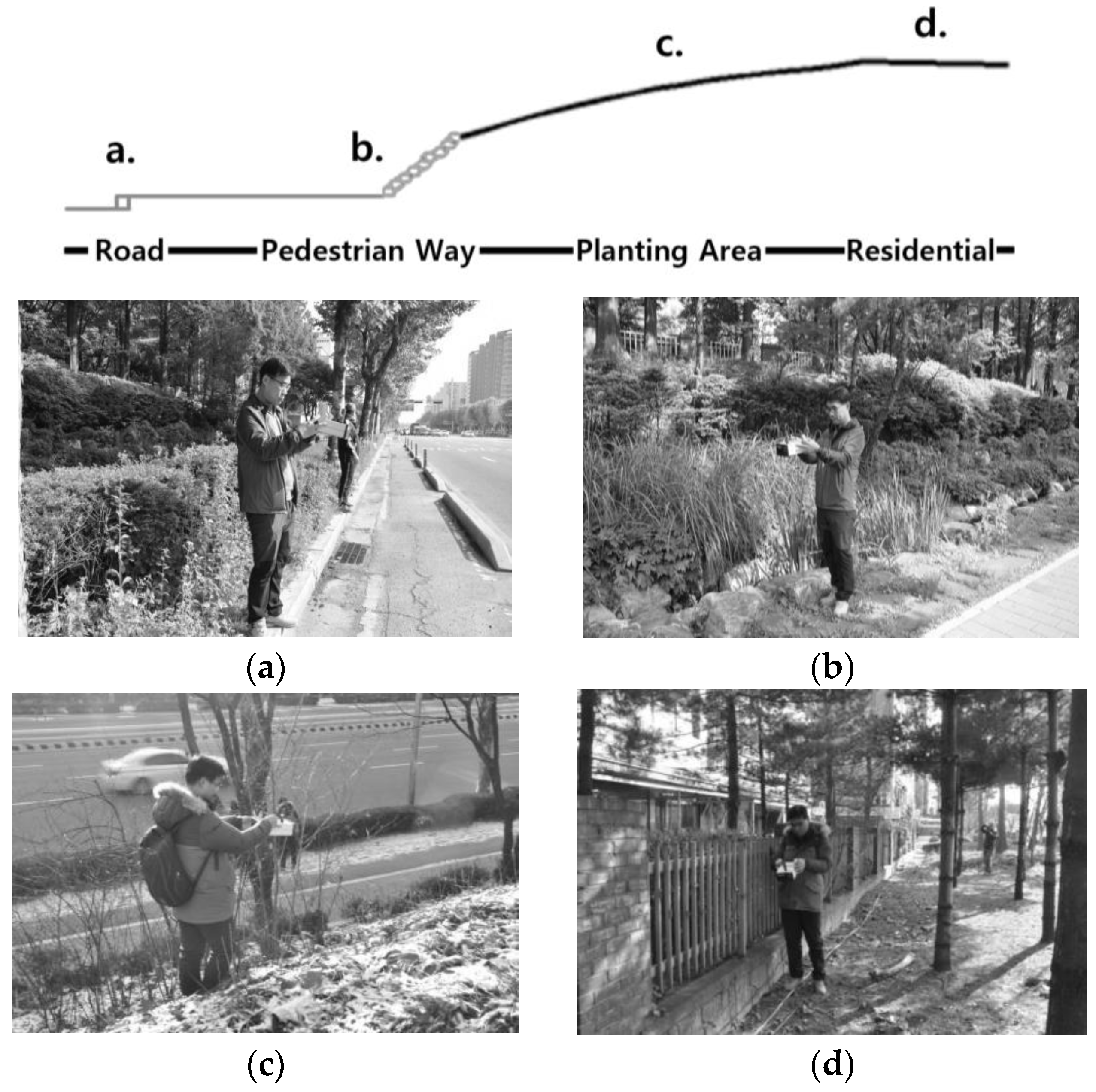
In the site survey, together with the AWS data, the Real-time Automated Measurement (RAM) method has been employed to measure the PM_2.5 concentration level. RAM method, also called β ray Absorption Method, can test the concentration levels of fine particles using β ray, fine, and vibration. In terms of choosing direct reading devices of fine particles, the study selected Air-Aide Model AA-3500 Airborne Particulate monitor supplied by Environmental Devices Corporation, which can measure and display the results immediately on site (

Table 5. Specifications of device (AA-3500).

Division	Information
Sensing range	0.001–20.0 mg/m3
PM size range	0.1–100 µm
Sampling flow rate	2.0 LPM
Alarm output	90 dB at 3 ft
Display	Real-Time mg/m3

). Every linear planting strip, cross-sectionally four spots of roadside, pedestrian way, planting area, and residential side—approximately 20 m—were tested with the device at approximately chest height (120 cm) for 4 s and repeated eight times (Figure 2).

The study also employed SPSS 21.0 to find the relationship between three-dimensional volumes and planting structures. One-way ANOVA was carried out with tree structures classified in single, double, and triple rows, and shrub structures divided into single, double, and multiple layers vertically. In particular, one-way ANOVA was employed to find seasonal differences of PM_2.5 and planting structures.

4. Results

The collected quantitative data could be divided into three areas, sloped, flat, and mounded, as per ground conditions of the planting areas. First, the three survey locations were identified as flat ground planting areas, as shown in Figure 3. The three survey locations also have three different planting types of single, double, and triple row of trees. Figure 4 and Figure 5 illustrate the sloped ground areas and the mounded ground areas.

Location 12 has the highest tree density, which led to highest PVPA and GVZ for trees, whereas Location 13 has the highest density, PVPA, and GVZ for shrub. Generally, higher shrub density sites showed lesser tree density, and, therefore, there is more space available for shrub planting as similar results could be found in the sloped ground condition sites. Single tree row planting site, Location 11, has the smallest GVZ quantity, whereas Location 12, where triple rows of tree planting exists, has the highest number of tree density, PVPA, and GVZ. For sloped ground areas, PVPA and GVZ showed quite similar results to each other, whereas PD values of trees and shrubs indicates opposite relationships, since it is found that more shrubs—or multiple layers of shrubs—is linked to higher PD values. The results of the mounded ground areas did not show much difference with flat and sloped ground conditions (

Table 6. Quantitative data per ground condition and planting structure type.

Locations	Ground	Planting Types (Row)	Planting Density (PD, %)		PVPA (m2)		GVZ (Grüvolumenzahl)
			Tree	Shrub	Tree	Shrub	Tree	Shrub
3	Sloped	Single	43.2	9.8	788.3	22.1	2.19	0.06
5			51.1	16.6	410.5	26.5	1.21	0.08
7			26	12	484.9	77.5	1.39	0.22
Sloped Ground and Single Row Average			40.1	12.8	561.23	42.03	1.6	0.12
1	Sloped	Double	77.9	5.6	1635.7	7.6	4.42	0.02
2			48.5	10.6	1077.3	19.8	2.76	0.05
6			68	7.4	1341.2	7.9	3.83	0.02
8			47.1	12.9	1826.1	23	5.37	0.07
9			26.8	11.8	604	22	1.78	0.06
10			73.2	5	1678.1	6.7	4.94	0.02
Sloped Ground and Double Row Average			56.9	8.9	1360.4	14.5	3.85	0.04
4	Sloped	Triple	36	13.1	604.3	34.4	1.59	0.09
Sloped Ground and Triple Row Average			49.8	10.5	1045.04	24.75	2.95	0.07
11	Flat	Single	48.1	8.5	257.9	9.8	1.07	0.04
12		Triple	56.7	22.3	606.2	37.2	2.09	0.13
13		Double	36.2	25.3	298.5	51.6	0.96	0.17
Flat Ground Average			47	18.7	387.5	32.9	1.37	0.11
15	Mounded	Double	73.9	5.8	4050.8	15.3	7.11	0.03
16			74.3	2.3	3934.1	6.6	6.91	0.01
Mounded Ground and Double Row Average			74.1	4.1	3992.5	11	7.01	0.02
14	Mounded	Triple	63.6	8.4	1106.3	23.6	2.04	1.39
Mounded Ground Average			70.6	5.5	3030.4	15.2	5.35	0.48

).

The winter survey was carried out on 14th January 2016 and it started at 07:30 a.m. when car traffic is peak due to prime commuting time. The day of the survey had temperatures of −8 to −1 °C, 24–49% humidity level, and wind speed of 1–2 m per second during the survey time. The winter survey indicates that the average concentration level of PM_2.5 was 55.5 µg/m³, the lowest was 17.0 µg/m³ and the highest was 114 µg/m³. On the other hand, the spring survey was carried out on 12 May 2016 and it started at 08:00 a.m. The day of the survey had temperatures of 2–22 °C, 45–60% humidity level, and wind speed of 1–4 m per second during the survey time. The spring survey indicates that the average concentration level of PM_2.5 was 38.6 µg/m³, the lowest was 18 µg/m³ (residential area) and the highest was 84 µg/m³ (roads) (

Table 7. PM_2.5 Concentration levels from the spring and winter survey.

Season	Location	Average (µg/m3)	Minimum (µg/m3)	Maximum (µg/m3)	AWS
Winter	1	48.3	29.0	63.0	07:30 a.m. 24 µg/m3
	2	65.3	54.0	78.0
	3	65.2	54.0	78.0
	4	34.7	25.0	51.0
	5	55.8	50.0	61.0	09:00 a.m. 24 µg/m3
	6	63.8	56.0	74.0
	7	53.8	48.0	66.0
	8	86.1	77.0	98.0	10:00 a.m. 45 µg/m3
	9	88.4	77.0	114.0
	10	70.7	57.0	93.0
	11	45.7	39.0	56.0	12:00 29 µg/m3
	12	57.8	49.0	67.0
	13	55.4	44.0	76.0
	14	28.3	17.0	41.0
	15	32.9	29.0	35.0	13:00 p.m. 24 µg/m3
	16	35.3	34.0	37.0
	Average	55.5	46.2	68.0	-
Spring	1	47.1	44.0	52.0	08:00 a.m. 19 µg/m3
	2	44.6	31.0	65.0
	3	30.1	18.0	59.0	09:00 a.m. 27 µg/m3
	4	38.3	32.0	47.0
	5	33.6	29.0	38.0
	6	41.9	27.0	67.0
	7	35.0	25.0	48.0	10:00 a.m. 14 µg/m3
	8	41.4	27.0	62.0
	9	29.7	22.0	40.0
	10	40.1	28.0	47.0	12:00 19 µg/m3
	11	44.4	33.0	58.0
	12	48.4	43.0	53.0
	13	57.0	39.0	84.0
	14	24.5	18.0	38.0	13:00 p.m. 14 µg/m3
	15	26.7	18.0	45.0
	16	35.4	27.0	42.0
	Average	38.6	28.0	52.8	-

).

Based on the winter and spring surveys, some comparisons can be made (Figure 6). Location 14 showed the lowest concentration levels in both spring and winter, whereas the highest concentration levels varies in seasons and locations. There are many seasonal changes at Locations 8 and 9. At Locations 4, 13, and 16, the concentration levels of spring survey were higher than that of winter survey; therefore, PD, PVPA, GVZ, seasonal and locational analyses are required. Average concentration levels of spring was 38.6 µg/m³, which is lower than that of winter (55.5 µg/m³). Previous research also claimed [38] that winter generally has lower value than the rest of the year.

In terms of differences per locations, such as roadside, pedestrian way, planting area, and residential area, the study results are illustrated in

Table 8. PM_2.5 concentration levels per location.

Location	Average Concentration Levels (µg/m3)
	Roadside		Pedestrian Way		Planting Area		Residential Area
	Winter	Spring	Winter	Spring	Winter	Spring	Winter	Spring
1	55	47.5	43.1	45.4	48.3	49.9	47	45.8
2	56.9	63	68.6	39.6	75.5	37.6	60.1	38.1
3	56.9	46.8	68.6	29.4	75.5	23.5	59.9	20.9
4	48.9	43.9	26.6	37.6	38.1	39.5	25.1	32.1
5	53.3	35.8	57	34	54.8	33.1	58.4	31.4
6	73.3	50.8	59.4	50.9	62.1	36.8	60.3	29.3
7	50.5	39.8	52.4	39.3	54.4	32.9	57.8	28.3
8	84.3	61.1	78.4	39.6	91.1	35.5	90.8	29.5
9	108.4	36.9	80.6	31.3	86.5	25.3	78.3	25.3
10	82.5	42	68.5	43.1	59	39	72.6	36.4
11	48.6	54.6	45	43.5	41.4	42.3	47.9	37.3
12	61.5	49.1	56.8	46.6	60.4	47.9	52.8	50.1
13	61.3	77	64.5	57.1	46.1	51.4	49.8	42.5
14	38.8	31.6	30.5	22.9	19.5	22.9	24.3	20.8
15	33.8	38.5	33.4	25.6	32.6	22.4	31.8	20.1
16	36.4	35.6	34.4	38.6	35.5	35.4	35.1	32
Average	59.4	47.1	54.2	39	55	35.9	53.2	32.5

.

The average PM_2.5 concentration levels in the winter decreased in the order of roadside, planting area, pedestrian way, and residential area, which, interestingly, indicates the planting area has higher concentration than the pedestrian way. In the spring, however, it decreases in the order of roadside, pedestrian way, planting area, and residential area. This is due to deciduous trees when the leaves are back in the spring. The filtering effects of deciduous trees in the spring provided much lower PM_2.5 concentration levels than in the winter.

5. Discussion

As a result of measuring the concentration of PM_2.5, this study found that it was 55.5 µg/m³ on average in winter, which was a harmful level according to the integrated environmental index provided by Seoul City, saying that levels above 50 µg/m³ may have harmful effect on sensitive groups of people. Particularly, the concentration of PM_2.5 was 38.6 µg/m³ on average in spring, which exceeded the mean concentration of PM_2.5 in Seoul City in 2015. The mean concentrations of PM_2.5 in every investigation spot were 46.6 µg/m³ for sidewalks, 45.5 µg/m³ for green spaces and 42.9 µg/m³ for residential areas, all of which were lower than 53.2 µg/m³ for roads, regardless of the season, and, especially, the concentration of PM_2.5 for residential areas was lowest. As seasonal characteristics, the concentration of PM_2.5 for green spaces (55.5 µg/m³) was higher than that for sidewalks (54.2 µg/m³) in winter, but, in spring, that for green spaces (35.9 µg/m³) became lower than that for sidewalks (39.0 µg/m³). As for the fluctuated concentration rate of fine particles in every investigation spot, the slope type showed an increase by 93.9% in winter, which was higher than the increased rate of the plain type (88.5%), and, in spring, the slope type showed a decrease by 69.5%, which was lower than the decreased rate of the plain type (75.1%).

Accordingly, this study confirmed that the slope ground type having the greatest tree green volume was more effective on reducing fine particles in spring, while the flat ground type having the most shrub green volume was more effective in winter, which indicates that the green volume of green buffers has great effect on the reduction of fine particles.

In the stage of confirming the effect of green buffers, this study analysed the correlation between the green volume of vegetation and the fluctuated rate of fine particles. As a result, it was found that the green coverage rate of trees and shrubs was related with the crown volume in every investigation spot, but they were mutually and complexly affected by each other.

As a result of analysing correlations between fluctuated concentration rate and the tree structure, this study found out that single row of trees showed the highest fluctuated concentration rate of PM_2.5 (84.77%), followed by double rows of trees (79.49%), and triple rows of trees (75.02%), indicating a negative correlation: the fluctuated concentration rate of PM_2.5 becomes lower with more rows of trees (

Table 9. Fluctuated concentration rate per tree structure.

	Division	N	Average (%)	SD (%)	SE (%)	Min. (%)	Max. (%)
Descriptive Statistics	Single Row	80	84.774	23.8102	2.6621	35.6	132.0
	Double Rows	144	79.493	19.4614	1.6218	44.3	124.4
	Triple Rows	32	75.022	16.0382	2.8352	45.1	100.0
	Total/Average	256	80.584	20.7211	1.2951	35.6	132.0
Test for Homogeneity of Variances	Levene Statistic	df 1		df 2		p-value
	6.211	2		253		0.002
Analysis of Variance	Division	SS	df	MS	F-ratio	p-value
	Between Groups	2565.695	2	1282.847	3.035	0.050
	Within Groups	106,921.883	253	422.616
	Total	109,487.578	255

).

Besides, as a result of analysing the effect of shrub structure, it was found that the single layer showed 88.79% in the fluctuated concentration rate, while the double layer and the multi-layer showed 81.16% and 68.93%, respectively. Therefore, this study concluded that more layers of shrubs are more effective at reducing the concentration of PM_2.5 (

Table 10. Fluctuated concentration rate per shrub structure.

	Division	N	Average (%)	SD (%)	SE (%)	Min. (%)	Max. (%)
Descriptive Statistics	Single Layer	32	88.788	19.664	3.4412	49.2	116.7
	Double Layers	192	81.160	19.4769	1.4056	44.3	132.0
	Triple Layers	32	68.925	24.5723	4.3438	35.6	116.7
	Total/Average	256	80.584	20.7211	1.2951	35.6	132.0
Test for Homogeneity of Variances	Levene Statistic	df 1		df 2		p-value
	2.258	2		253		0.107
Analysis of Variance	Division	SS	df	MS	F-ratio	p-value
	Between Groups	2565.695	2	1282.847	3.035	0.050
	Within Groups	106,921.883	253	422.616
	Total	109,487.578	255

).

As for seasonal characteristics, this study analysed the correlation between the concentration of PM_2.5 for residential areas in winter and the green coverage rate of each green space type. As a result, this study found out that there was a negative correlation, showing that the higher the shrub green coverage rate is, the lower the concentration value becomes in all ground types—slope, flat, and mounded. Moreover, based on the ground types of residential area, a one-way ANOVA has been carried out in the winter as shown in

Table 11. Concentration rate per ground condition within residential area in winter.

	Ground Types	N		Average (µg/m3)	Min. (µg/m3)	Max. (µg/m3)
Descriptive Statistics	Sloped	80		61.0125	23.00	97.00
	Flat	24		50.1250	45.00	56.00
	Mounded	24		30.3750	23.00	36.00
	Total/Average	128		47.1708	30.33	63.00
Test for Homogeneity of Variances	Levene Statistic	df1		df2		p-value
	13.276	2		125		0.000
Analysis of Variance	Division	SS	df	MS	F-ratio	p-value
	Between Groups	17,613.192	2	8806.596	45.846	0.000
	Within Groups	24,011.238	125	192.090
	Total	41,624.430	127

,

Table 12. Descriptive statistics for concentration rate per ground condition in winter.

Division	Green Coverage Rate of Shrubs (%)	N	Average (%)	SD (%)	SE (%)	Min. (%)	Max. (%)
Flat	8.5	8	98.763	5.4636	1.9317	87.5	104.3
	22.3	8	86.075	4.5594	1.6120	81.3	92.7
	25.3	8	81.425	3.8788	1.3714	73.6	86.2
	Total/Average	24	88.754	4.6339	1.6383	80.8	94.4
Slope	5.0	8	88.213	3.5926	1.2702	80.6	92.6
	5.6	8	85.700	5.5577	1.9650	79.7	97.8
	7.4	8	82.238	1.5203	0.5375	80.8	85.1
	11.8	8	72.288	2.7441	0.9702	68.8	77.2
	13.1	8	51.700	5.5918	1.9770	45.1	60.5
	Total/Average	40	76.027	3.8013	1.3439	71.0	82.6
Mounded	2.3	8	96.613	3.1425	1.1111	91.9	100.0
	5.8	8	94.175	5.4255	1.9182	85.3	103.1
	8.4	8	62.863	6.0264	2.1306	56.1	71.4
	Total/Average	24	84.550	4.8648	1.7199	77.7	91.5

and

Table 13. Analysis of variance for concentration rate per ground condition in winter.

Division		SS	df	MS	F-Ratio	p-Value
Flat	Between Groups	1288.491	2	644.245	29.425	0.000
	Within Groups	459.789	21	21.895
	Total	1748.280	23
Slope	Between Groups	7091.284	4	1772.821	104.400	0.000
	Within Groups	594.336	35	16.981
	Total	7685.620	39
Mounded	Between Groups	5667.937	2	2833.969	112.416	0.000
	Within Groups	529.402	21	25.210
	Total	6197.340	23

.

All the factors affecting the reduction of fine particles were related to the green space coefficient (m³/m²) through the green coverage rate (%) as a meaning of area and the green volume (m³) as a meaning of bulk, and they were also affected by the complex structure of trees and shrubs. Thus, this study confirmed that the number of tree rows and the number of shrub layers have negative correlations with the fluctuated concentration rate of PM_2.5. Especially, it was judged that the shrub green volume has greater effect than any other factor, and each green space type shows a negative correlation with the shrub coverage rate in winter (Table 12 and Table 13).

Overall, the paper investigated the concentration levels of PM_2.5 in roadsides, planting areas, and residential zones and attempted to identify any significant factors influencing the lessening of PM_2.5. After the survey in winter and spring, it was found that there was serious PM_2.5 concentration levels in the areas of pedestrian paths, planting, and residential areas compared to other urban areas, especially, a substantially lower level of PM_2.5 concentrations were revealed in the residential areas located behind planting bands as green buffer.

The concentration levels of PM_2.5 are generally surveyed to be higher in winter than spring. However, the concentration levels of PM_2.5 decreases in the order of planting areas, pedestrian ways, and residential areas in winter, whereas, it decreases in the order of pedestrian ways, planting areas, and residential areas in spring. There was clear variation of PM_2.5 concentration levels seasonally due to the leaves in vegetation. In terms of ground condition, because of the three-dimensional volumes of tree and shrubs, the sloped planting areas had better performance than flat areas at reducing PM_2.5 levels in spring, whereas, the flat area of vegetation had lower PM_2.5 levels in winter.

Quantitatively speaking, planting coverage rate and three-dimensional volume is critical to influence the concentration level of PM_2.5; however, qualitative factors are planting types and structures. In particular, the existence of shrub planting bands was a key factor to reduce the density of PM_2.5, which led to concluding that creating multi-layered shrub planting is the most effective way of reducing PM_2.5 levels. In some tree planting cases, too many overlapping planning centres between trees can cause blocking PM_2.5 diffusions into the air, which increases the concentration level of PM_2.5. Therefore, leaving sufficient gaps among trees is recommended.

6. Conclusions

Thus far, a number of studies has been carried out to resolved the health risk hazards of PM_2.5; however, the methods using urban trees planting schemes are relatively unexplored in South Korea, despite urban trees being considered green lungs within larger cities. Therefore, this study aimed to explore the effects of planting buffers as the reduction methods of fine particles (PM_2.5) in urban areas. Moreover, it analysed the changes of fine particle concentration levels by planting structures, green volumes and planting types of roadside green buffers. A case study was employed as a research methodology, where 16 survey locations on three main streets in Seoul that indicated the highest PM_2.5 emissions per year based on Seoul statistics were chosen.

The findings are summarized in the previous section; however, notably, the quantitative factors affecting on the concentration level of PM_2.5 were planting coverage rate and three-dimensional volume of plants, whereas, planting types (including ground conditions) and structures are highly influential qualitatively. The most effective urban planting structures for reducing the concentration level of PM_2.5 were triple rows of tree planting and multiple layers of shrub structure. Similarly, the plant coverages of shrubs and PM_2.5 concentration level have a negative correlation in all ground conditions. Moreover, shrub plantings play critical role in reducing the density of PM_2.5. It is also found that dense tree planting did not guarantee the reduction of PM_2.5 since more gap among trees allow the diffusion PM_2.5 in the air, thus sufficient gap is required for trees to reduce fine particles in larger cities.

However, this study could not include all environmental variables within urban areas; moreover, the surveys were only carried out in two seasons, spring and winter, when critical changes occur due to leaves in plants. Further research needs to be carried out to investigate some important factors, such as efficiency comparison between evergreen and deciduous, screening planting distance from PM_2.5 sources, and planting species variations in the future.

Currently, relevant legislations only deal with planting width and plan coverage rate in South Korea, which is not enough to reduce the threats from PM_2.5 systematically at the national level. This study found the critical factors of urban planting for reduction of PM_2.5 are three-dimensional volumes and quantity of planting bands (rows). In particular, trees need to be planted at certain distance to not trap any PM_2.5 and for free movement of winds, and more shrub planting is required to increase three-dimensional volume of urban plantings.

References

- Goswami, A.; Barman, J.; Rajput, K.; Lakhlani, H.N. Behaviour Study of Particulate Matter and Chemical Composition with Different Combustion Strategies. Available online: http://papers.sae.org/2013-01-2741/ (accessed on 21 September 2017).
- Park, D.-U.; Ha, K.-C. Characteristics of PM10, PM2.5, CO2 and CO monitored in interiors and platforms of subway train in Seoul, Korea. Environ. Int. 2008, 34, 629–634. [Google Scholar] [CrossRef] [PubMed]
- Boldo, E.; Medina, S.; le Tertre, A.; Hurley, F.; Mücke, H.-G.; Ballester, F.; Aguilera, I. Apheis: Health impact assessment of long-term exposure to PM2.5 in 23 European cities. Eur. J. Epidemiol. 2006, 21, 449–458. [Google Scholar] [CrossRef] [PubMed]
- Chow, J.C.; Watson, J.G.; Edgerton, S.A.; Vega, E. Chemical composition of PM2.5 and PM10 in Mexico City during winter 1997. Sci. Total Environ. 2002, 287, 177–201. [Google Scholar] [CrossRef]
- Harrison, R.M.; Deacon, A.R.; Jones, M.R.; Appleby, R.S. Sources and processes affecting concentrations of PM10 and PM2.5 particulate matter in Birmingham (UK). Atmos. Environ. 1997, 31, 4103–4117. [Google Scholar] [CrossRef]
- Kang, C.-M.; Sunwoo, Y.; Lee, H.S.; Kang, B.-W.; Lee, S.-K. Atmospheric concentrations of PM2.5 trace elements in the Seoul urban area of South Korea. J. Air Waste Manag. Assoc. 2004, 54, 432–439. [Google Scholar] [CrossRef] [PubMed]
- Park, E.-J.; Kim, D.-S.; Park, K. Monitoring of ambient particles and heavy metals in a residential area of Seoul, Korea. Environ. Monit. Assess. 2008, 137, 441–449. [Google Scholar] [CrossRef] [PubMed]
- Seo, Y.-H.; Ku, M.-S.; Choi, J.-W.; Kim, K.-M.; Kim, S.-M.; Sul, K.-H.; Jo, H.-J.; Kim, S.-J.; Kim, K.-H. Characteristics of PM2.5 Emission and Distribution in a Highly Commercialized Area in Seoul, Korea. J. Korea Soc. Atmos. Environ. 2015, 31, 97–104. [Google Scholar] [CrossRef]
- Wilson, A.M.; Salloway, J.C.; Wake, C.P.; Kelly, T. Air pollution and the demand for hospital services: A review. Environ. Int. 2004, 30, 1109–1118. [Google Scholar] [CrossRef] [PubMed]
- Chang, C.-C.; Tsai, S.-S.; Ho, S.-C.; Yang, C.-Y. Air pollution and hospital admissions for cardiovascular disease in Taipei, Taiwan. Environ. Res. 2005, 98, 114–119. [Google Scholar] [CrossRef] [PubMed]
- Hart, J.E.; Laden, F.; Schenker, M.B.; Garshick, E. Chronic obstructive pulmonary disease mortality in diesel-exposed railroad workers. Environ. Health Perspect. 2006, 114, 1013–1017. [Google Scholar] [CrossRef] [PubMed] [Green Version]
- Hänninen, O.O.; Palonen, J.; Tuomisto, J.T.; Yli-Tuomi, T.; Seppänen, O.; Jantunen, M.J. Reduction potential of urban PM2.5 mortality risk using modern ventilation systems in buildings. Indoor Air 2005, 15, 246–256. [Google Scholar] [CrossRef] [PubMed]
- Turpin, B.J.; Lim, H.-J. Species contributions to PM2.5 mass concentrations: Revisiting common assumptions for estimating organic mass. Aerosol Sci. Technol. 2001, 35, 602–610. [Google Scholar] [CrossRef]
- Yu, L.; Wang, G.; Zhang, R.; Zhang, L.; Song, Y.; Wu, B.; Li, X.; An, K.; Chu, J. Characterization and source apportionment of PM2.5 in an urban environment in Beijing. Aerosol Air Qual. Res. 2013, 13, 574–583. [Google Scholar] [CrossRef]
- Mohapatra, K.; Biswal, S. Effect of particulate matter (PM) on plants, climate, ecosystem and human health. Int. J. Adv. Technol. Eng. Sci. 2014, 2, 2348–7550. [Google Scholar]
- Climate Atmospheric Research Team. PM2.5 emission factor report – Estimation of air pollutant emissions in 2011. National Institute of Environmental Research: Seoul, Korea. Available online: http://webbook.me.go.kr/DLi-File/NIER/09/019/5568844.pdf (accessed on 21 September 2017).
- Bae, H.-J. Effects of Short-term Exposure to PM10 and PM2.5 on Mortality in Seoul. Korea J. Environ. Health Sci. 2014, 40, 346–354. [Google Scholar]
- Hamra, G.B.; Guha, N.; Cohen, A.; Laden, F.; Raaschou-Nielsen, O.; Samet, J.M.; Vineis, P.; Forastiere, F.; Saldiva, P.; Yorifuji, T. Outdoor particulate matter exposure and lung cancer: A systematic review and meta-analysis. Environ. Health Perspect. 2014, 122, 906–911. [Google Scholar] [CrossRef] [PubMed]
- Raaschou-Nielsen, O.; Andersen, Z.J.; Beelen, R.; Samoli, E.; Stafoggia, M.; Weinmayr, G.; Hoffmann, B.; Fischer, P.; Nieuwenhuijsen, M.J.; Brunekreef, B.; et al. Air pollution and lung cancer incidence in 17 European cohorts: Prospective analyses from the European Study of Cohorts for Air Pollution Effects (ESCAPE). Lancet Oncol. 2013, 14, 813–822. [Google Scholar] [CrossRef]
- Haywood, J.; Boucher, O. Estimates of the direct and indirect radiative forcing due to tropospheric aerosols: A review. Rev. Geophys. 2000, 38, 513–543. [Google Scholar] [CrossRef]
- Cohen, A.J.; Anderson, H.R.; Ostro, B.; Pandey, K.D.; Krzyzanowski, M.; Künzli, N.; Gutschmidt, K.; Pope, A.; Romieu, I.; Samet, J.M. The global burden of disease due to outdoor air pollution. J. Toxicol. Environ. Health Part A 2005, 68, 1301–1307. [Google Scholar] [CrossRef] [PubMed]
- Pope, C.A.; Bhatnagar, A.; McCracken, J.P.; Abplanalp, W.; Conklin, D.J.; O’Toole, T. Exposure to Fine Particulate Air Pollution Is Associated with Endothelial Injury and Systemic InflammationNovelty and Significance. Circ. Res. 2016, 119, 1204–1214. [Google Scholar] [CrossRef] [PubMed]
- Pope, C.A., III; Burnett, R.T.; Thun, M.J.; Calle, E.E.; Krewski, D.; Ito, K.; Thurston, G.D. Lung cancer, cardiopulmonary mortality, and long-term exposure to fine particulate air pollution. JAMA 2002, 287, 1132–1141. [Google Scholar] [CrossRef] [PubMed]
- Twomey, S. The influence of pollution on the shortwave albedo of clouds. J. Atmos. Sci. 1977, 34, 1149–1152. [Google Scholar] [CrossRef]
- Cesaroni, G.; Forastiere, F.; Stafoggia, M.; Andersen, Z.J.; Badaloni, C.; Beelen, R.; Caracciolo, B.; de Faire, U.; Erbel, R.; Eriksen, K.T. Long term exposure to ambient air pollution and incidence of acute coronary events: Prospective cohort study and meta-analysis in 11 European cohorts from the ESCAPE Project. BMJ 2014, 348, f7412. [Google Scholar] [CrossRef] [PubMed]
- Nawrot, T.S.; Perez, L.; Künzli, N.; Munters, E.; Nemery, B. Public health importance of triggers of myocardial infarction: A comparative risk assessment. Lancet 2011, 377, 732–740. [Google Scholar] [CrossRef]
- Hogan, C.M. Abiotic Factor in Encyclopedia of Earth; National Council for Science and Environment: Washington, DC, USA, 2010. [Google Scholar]
- Kim, J.-H.; Oh, D.-K.; Yoon, Y.-H. Evaluation of Noise Decreasing Effects by Structures in Roadside Buffer Green. J. Environ. Sci. Int. 2015, 24, 647–655. [Google Scholar] [CrossRef]
- National Institute of Environmental Research. Annual Report of Air Quality in Korea. Korea Ministry of Environment: Seoul, Korea, 2015; pp. 346–348. Available online: http://webbook.me.go.kr/DLi-File/NIER/09/022/5618423.pdf (accessed on 21 September 2017).
- Perini, K.; Ottelé, M.; Fraaij, A.L.A.; Haas, E.M.; Raiteri, R. Vertical greening systems and the effect on air flow and temperature on the building envelope. Build. Environ. 2011, 46, 2287–2294. [Google Scholar] [CrossRef]
- Ottelé, M.; van Bohemen, H.D.; Fraaij, A.L.A. Quantifying the deposition of particulate matter on climber vegetation on living walls. Ecol. Eng. 2010, 36, 154–162. [Google Scholar] [CrossRef]
- Perini, K.; Ottelé, M.; Giulini, S.; Magliocco, A.; Roccotiello, E. Quantification of fine dust deposition on different plant species in a vertical greening system. Ecol. Eng. 2017, 100, 268–276. [Google Scholar] [CrossRef]
- Nowak, D.J.; Crane, D.E.; Stevens, J.C. Air pollution removal by urban trees and shrubs in the United States. Urban For. Urban Green. 2006, 4, 115–123. [Google Scholar] [CrossRef]
- Simon, E.; Braun, M.; Vidic, A.; Bogyo, D.; Fabian, I.; Tothmeresz, B. Air pollution assessment based on elemental concentration of leaves tissue and foliage dust along an urbanization gradient in Vienna. Environ Pollut. 2011, 159, 1229–1233. [Google Scholar] [CrossRef] [PubMed]
- Yang, G.-S. The Influence of Resident Satisfaction Regarding Buffer Green Space at Meoyng-ji Multi-family Housing in Busan Metropolitan City. J. Korea Inst. Landsc. Archit. 2013, 41, 38–45. [Google Scholar] [CrossRef]
- Jeon, B.-I. Meteorological Characteristics of the Wintertime High PM10 Concentration Episodes in Busan. J. Environ. Sci. Int. 2012, 21, 815–824. [Google Scholar] [CrossRef]
- Kim, S.D. Ultrafine Particles in Korea; University of Seoul: Seoul, Korea, 2010. [Google Scholar]
- Kim, S.D.; Kim, C.W. Physio-Chemical Characteristics of Ultrafine Particles in Seoul Area; Seoul Urban Studies: Seoul, Korea, 2008; Volume 9, pp. 23–33. [Google Scholar]
- Schulze, H.; Pohl, W.; Grossmann, M. GrÜnvolumenzahl GVZ und Bodenfunktionszahl BFZ in der Landschafts -und Bauleitplanung; Behörde für Bezirksangelegenheiten, Naturschutz und Umweltgestaltung. Available online: http://www.isebek-initiative.de/uploads/sn/FHH_UB_1987_Gruenvolumen-und-Bodenfuktionszahl.pdf (accessed on 21 September 2017).
Figure 1.
Map of survey location.
Figure 2.
Tested location and reading posture of PM2.5: (a) road; (b) pedestrian way; (c) planting area; and (d) residential.
Figure 3.
Typical plan and section of flat ground: (a) single row planting (Location 11); (b) Double rows planting (Location 12); and (c) triple rows planting (Location 13). (GB: Green Buffer; PW: Pedestrian Way; and RB: Road Bikes).
Figure 4.
Typical plan and section of sloped ground: (a) single row planting (Locations 3, 5, 7); (b) double rows planting (Locations 1, 2, 6, 8, 9, 10); and (c) triple rows planting (Location 4). (GB: Green Buffer; PW: Pedestrian Way; RB: Road Bikes; and SL: Slope).
Figure 5.
Typical plan and section of mounded ground: (a) double rows planting (Locations 15, 16); and (b) triple rows planting (Location 14). (GB: Green Buffer; PW: Pedestrian Way; and RB: Road Bikes).
Figure 6.
Seasonal differences of PM2.5 concentration levels.