Investment Strategy in a Closed Loop Supply Chain: The Case of a Market with Competition between Two Retailers


Business School, Kwangwoon University, 26 Kwangwoon-gil (447-1, Wolgye-dong), Nowon-Gu, Seoul 139-701, Korea
*
Author to whom correspondence should be addressed.
Sustainability 2017, 9(10), 1712; https://doi.org/10.3390/su9101712
Submission received: 11 August 2017
/
Revised: 18 September 2017
/
Accepted: 21 September 2017
/
Published: 25 September 2017
(This article belongs to the Special Issue Reverse Logistics: An Interdisciplinary Approach)
Abstract
:To survive in the ceaseless cycle of competition, businesses have developed strategies to become sustainable. These strategies include reusing products, which can lead not only to the creation of economic benefits but also to improvements in a corporation’s social and environmental responsibility. Product reuse can also increase the profit earned on new products by compensating customers who bring in old products to buy new ones, as the ensuing remanufacturing process allows for the reuse of materials and thus drives down costs. As businesses have come to recognize these values, the marketing competition to retrieve used products from customers has intensified. This research focuses on identifying effective compensation strategies to determine the appropriate advertising investment and trade-in value in a market where two homogeneous retailers compete. Retailers advertise to secure more customers to trade in their used products and to generate more trade-in sales than competitors do. A retailer’s results may vary according to its competitor’s investment strategy, which makes it useful to employ information on past competitor investment patterns to plan future investment strategies. However, as competitors using one another’s information may intensify the competition, better investment results could be obtained by ignoring competitor investment information. Therefore, this study suggests four competition strategies that determine the advertisement costs and trade-in allowance spent by retailers and discusses the difference in the profits obtained by the retailers under each of the four strategies.

1. Introduction
As the importance of recovering used products in a closed loop supply chain (CLSC) has increased, diverse marketing strategies have emerged to promote customer retention.
CLSCs can offer economic benefits in two ways: first, by reducing businesses’ operating costs. Used products retrieved from the customer undergo a remanufacturing process and are then resold in a forward supply channel; alternatively, only select, usable parts may be set aside to be incorporated into new products. Thus, employing used products can reduce the amount of raw materials required in traditional manufacturing processes, which ultimately reduces the operating cost.
The second economic benefit of CLSCs is that they can create the potential for new product sales. Many corporations currently offer a trade-in option, whereby customers who bring in used products are provided trade-in allowances that can be applied toward the purchase of new products [1]. Such trade-in sales can lead customers to buy new products and increase demand.
For example, in February 2011, Best Buy launched its “Buy Back” program. When purchasing a new product at Best Buy, each customer was provided with the option to participate in the program by paying a prespecified and nonrefundable fee that depends on the product category and purchase price of the product. Each participant could return an old product within two years and receive a prespecified trade-in value for purchasing new electronic equipment. Xerox, whose remanufacturing facility is based partly on returns from trade-ins, experienced cost savings of several hundred million dollars each year [2,3]. There are similar examples from industries such as computers (e.g., IBM’s Global Asset Recovery Services; see www.pprc.org), furniture, carpets, power tools, and refrigerators [2,3,4].
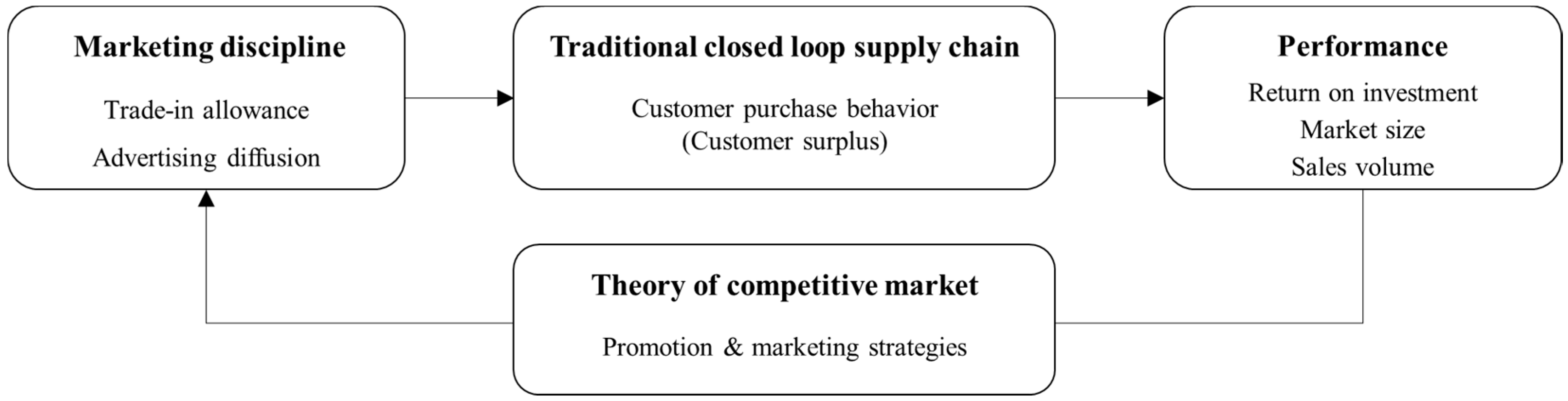
While a large part of the CLSC literature focuses on operational decisions, a small but significant research stream has explored sustainability decisions in a supply chain from a marketing perspective according to the market structure (competitive situation) [5,6]. The following three issues have been examined: (i) How does the retailers’ subsidy affect switching by customers? (ii) How does advertising affect information diffusion and awareness? (iii) How do classical marketing decisions such as advertisement and the subsidy amount, relate to retailers’ return volume of used products and opportunity to obtain new product sales? We do so by integrating four district theories—consumer’s surplus [7,8], trade-in allowances [9,10], adverting diffusion [11,12], and the theory of competitive markets [13,14]—to advance research propositions that might begin to guide the development of the interdisciplinary field of sustainability.
We chose these four perspectives to build our framework of sustainable supply chain management (SSCM) because each theoretical base is derived from a different discipline. These four theories were selected because while each offers unique perspectives, they are also complementary in allowing for an expansion of SSCM from a marketing perspective, as shown in Figure 1.
Retailers make investments in advertising to promote their trade-in sales programs to a larger number of customers and offer additional trade-in allowances to win competitions against rivals. The outcomes of such investments depend on the investment strategies employed by a retailer’s competitors. Consider, for example, retailer A that invests more in advertisement and retailer B that spends more money on trade-in allowances. Which of the two retailers will generate a higher profit? Retailer A will be able to more widely disseminate information on its trade-in sale program, which will increase the number of customers who are aware of about both retailers, and these customers will choose the retailer that offers the higher trade-in value. Thus, retailer A, which offers a lower trade-in value than retailer B, may experience a smaller effect from its advertisement. However, there is a case in which retailer A can profit more. Because retailer B spends less on advertisement, the number of customers who know of both retailers would not be as high, and if retailer A can increase the number of customers who know only about retailer A, it will be able to subsequently increase the effect of its advertisement and generate profit despite those customers who know about both retailers and shop with retailer B. In the same manner, retailer B’s profits will depend on the amount of money that retailer A spends on investment or trade-in allowances. The outcome of an investment made by a retailer is highly dependent on the investment strategies of its competitors. Thus, determining one’s investment strategy using competitors’ past investment information can lead to a profitable outcome. However, if one company can use its competitors’ past investment information, its competitors can similarly use that company’s information. As there is a possibility that competition will intensify in this case, establishing an investment strategy based on own information while ignoring competitor information may lead to a better result.
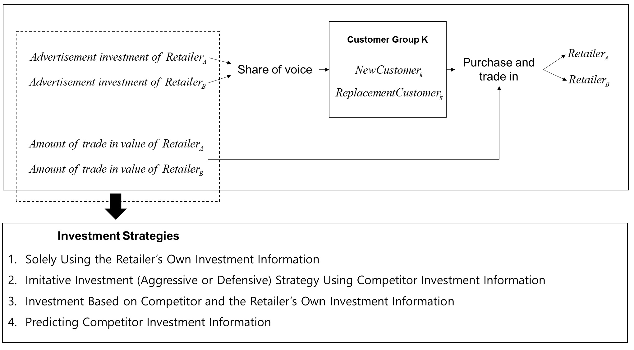
This study examines how two homogenous retail companies that operate in a duopolistic competitive setting determine their investment on advertisement and trade-in values for used products to encourage customers to use their trade-in sale programs. The study then establishes a strategy for determining the amount of investment required to beat the competition and proposes four competitive strategies based on whether competitor investment information is considered. The four strategies are (1) investment based solely on own investment information; (2) imitative (aggressive or defensive) investment using the competitor’s investment information; (3) investment based on a combination of competitor and own investment information; and (4) investment based on a prediction of competitor investment information. This study analyzes the effect of these four investment strategies on the profits of the two retailers.
2. Literature Review
For the past two years, studies in this field have sought to resolve basic issues in the supply chain to establish the foundation of a CLSC [15]. Most studies on CLSCs have focused on problems from an operational perspective, determining effective reserve-channel designs, finding the optimal price, and collaboration among supply chain participants [16,17,18,19,20,21,22,23,24,25,26,27,28,29].
Several studies have suggested that customers are presented with a variety of incentive strategies to encourage the collection of used products. Savaskan et al. [21] addressed the selection of an effective product retrieval design in a CLSC and model the response of consumers who have an incentive for used products in the form of response functions used in the adverting response models of consumer retention and product awareness. Mafakheri and Nasiri [26] considered the retrieval rate of printer ink cartridges by determining customer incentives based on the difference between the retail price of a new cartridge and the refilling price. Govindan and Popiuc [27] studied the collaborative relationship between the retailer and manufacturer in the computer remanufacturing industry. They considered a linear relationship between the amount of investment in retrieval activity and the rate of used product retrieval.
However, customers receiving compensation for trading in their used product and purchasing a new one is a critical element that directly affects the profits of companies participating in a CLSC. It is not a simple matter to express and understand this issue because the product preferences of customers, the remaining value of the returned used product, promotional competition among retailers, the retail price, the recycling value, and many other elements all affect it.
In contrast to studies on CLSCs, studies on the trade-in value, which focus on the marketing strategies applied to customers, examine customer characteristics in determining the retrieval rate. The objective of a CLSC in retrieving used products is not only to generate profits via the recycling value of the old goods but also to encourage customers to return to the store and purchase new products. In calculating the probability that a replacement customer will purchase a new product after bringing in a used one for trade-in, Ray et al. [7] employ the remaining value of the retrieved used product, reservation price, and customer surplus, which is affected by the trade-in allowance offered by the retailer. Ray et al. [7] assumed that customers’ reservation prices for products sold by the retailer follow a uniform distribution, and they determined the reservation prices and the scope of customers who benefit from a trade-in sale program based on the remaining value of the retrieved used product. Koçaş and Bohlmann [30] studied pricing strategy in a market with two large bookstores and one small bookstore and segmented customers into types with respect to brand loyalty and price sensitivity. By segmenting the customers, they were able to propose pricing strategies that explain customer behaviors in a more realistic manner. Yin and Tang [31] developed a model in which customers pay an up-front fee to register for a trade-in sale program that offers compensation allowances. They also considered segmented customer groups and how to consider the trade-in allowance, the price of used products in the used goods market, the retail price, and the reservation price in making the optimal purchase decision. In accordance with this trend in the literature, the present study proceeds on the assumption that considering realistic customer behaviors in CLSC studies can further advance the field.
In addition, promotion strategies employed by individual retailers to encourage the trade-in of used products can pose significant threats to competitors via influencing the product retrieval rate, which is directly linked to retailer profits. Rajib et al. [32] studied the advertisements employed by two companies with two different levels of service quality and the firms’ promotion strategies for discount prices. The current study explores, the impact of customer characteristics, such as shopping cost, preference for service, and store switching cost, on the frequency of advertisement and the level of discount for companies with different service quality levels. Joshi et al. [33] studied promotion strategies related to the product line; developing intrinsic value in the minds of customers is at the core of corporate marketing strategy, which Joshi et al. define as a firm’s “home turf”. The intensity of competition between businesses depends on whether each company intends to respect its competitors’ turf or expand operations to encroach on it. Delre et al. [34] studied the competition strategy of distributors in the movie industry, examining their initial advertising costs and investment in films. In their model, viewers (who each have different preferences over movies) attend the theater during the launch and post-launch periods.
Some of CLSC studies have covered the Corporate Social Responsibility (CSR) and the sustainability as well as economic side of firms. With the major issue of CSR which includes environmental, ethical, legal and philanthropic dimension [35,36,37], many firms are strategically transforming their supply chain into the CLSC [38] and the government enlarges a public procurement to bring about the sustainability [39]. However, the social responsibility and economic goals of firms have been pitted against each other, yet the two are decidedly interdependent [40]. Although the previous CLSC studies are mainly belonged to the economic side of firms, the achievement of sustainability through CLSC forces the researchers the challenge that meets the demands of the environment and the society while satisfying firm’s economic growth.
3. Model Development
Before providing details about the model considered in this study, below, we define the terms used in the model.
| Index | |
| investment decision period of retailers, | |
| retailer A, retailer B both retailers | |
| competitor | |
| customer group based on the distance | |
| product age of replacement customer, | |
| Terms | |
| new customer who know information about retailer r in customer group k | |
| replacement customer who have existing product and know information about retailer r in group k in period t | |
| maximum length of use for the product, thus is the remaining useful lifespan at period t | |
| reservation price of customers in group k that differs among individuals for retailer r in period t, | |
| the maximum price that customer is willing to pay for retailer t’s the product in period t | |
| retail price of retailer r | |
| purchase probability that new customers who know information about one retailer in period t | |
| purchase probability that new customers who know information about both retailers in period t | |
| probability that replacement customers in group k who have existing product and know information about one retailer purchase retailer r’s product in period t | |
| probability that replacement customers in group k who have existing product and know information about both retailers purchase retailer r’s product in period t | |
| recycling value of existing products collected from replacement customers | |
| total profit of retailer r in period t | |
| subsidy offered by retailer r for existing products to replacement customers in period t | |
| predicted subsidy offered by competitors r–j for existing product to replacement customers in period t | |
| advertising investment of retailer r for existing products held by replacement customers in period t | |
| predicted advertising investment by competitor r–j for existing products held by replacement customers in period t | |
| ratio of profit increase/decrease in period t, | |
| maximum subsidy offered by retailer r for existing products held by any replacement customer | |
| maximum advertising investment by a retailer r for any customer | |
| basic retailer incentive ratio for any customer | |
| advertisement effect of customer group k on retailer r in period t | |
| distance weight factor of customer group k on retailer r |
3.1. Retailers
Rajiv et al. [32] define vertical and horizontal differentiation by retailers as follows: Vertical differentiation occurs when different retailers are located in different positions in terms of their product quality. For example, if the quality of a product sold by retailer H is , and the quality of the products offered by retailer L is , the two companies are vertically differentiated if > > 0. In contrast, horizontal differentiation occurs when different retailers use their relative advantages to induce customers to purchase products. Advantages enjoyed by retailers that attract customers include the following: (1) familiarity with the layout of the company; (2) previous experience with the services or assistance offered by the company; (3) familiarity with products or prices offered by the company; and (4) geographical and locational advantages.
The model in this study considers retail companies competing with comparable merchandise: While the products sold by retailer A and retailer B are not different in terms of price or quality (no vertical differentiation), the companies are separated geographically (horizontal differentiation). Therefore, if a customer does not have information about one company, or the discount offered by the other company, he or she uses the closer retailer. For example, customers located closer to retailer A mainly use that company, while those closer to B usually shop at retailer B. If each retailer makes an investment to promote its products, it can attract customers that would otherwise have visited its competitor. The model considers the promotions that retailers offer on their products that target returning customers. Each retailer determines its advertising cost and trade-in allowance during every decision-making cycle to encourage returning customers to trade in their used goods.
3.2. Customer Structure
This study categorizes customers into two types: the group of new customers (NCs) who do not currently own a used product and may or may not purchase a new product and replacement customers (RCs) who may decide to purchase a new product at a discounted price after turning in their old product or may continue using their old product.
The model assumes that customers of these two types are distributed uniformly between and around the two retailers. As shown in Figure 2, the two retailers are located at the edges of a straight line, with new and replacement customers coexisting within the five customer groups in between the retailers. The size of new and replacement customer types in each customer group k (k = 1, 2, 3, 4, 5 here) are defined as , and the two types of customers act independently from one another.
Advertisement is a critical element in a market economy. Even if a retail company provides a large trade-in allowance, a purchase will not occur if customers are not aware of the sale information. Thus, advertisements promote awareness of the prices of new products and inform replacement customers of the trade-in allowances offered as a part of a trade-in sale program. A regular durable goods market features advertisements using physical and offline media, such as leaflets, and thus, we assume that customers located closer to a retailer engaged in advertising will experience a larger effect from the promotion campaign.
Delre et al. [34] studied the effect of initial advertising campaigns for movies and calculated the effect of the advertisement by dividing the square root of the advertising cost by the difference between the film movie and viewer preference. The current study defines the effect of the investment made by retailer r to advertise to customer group k as in (1).
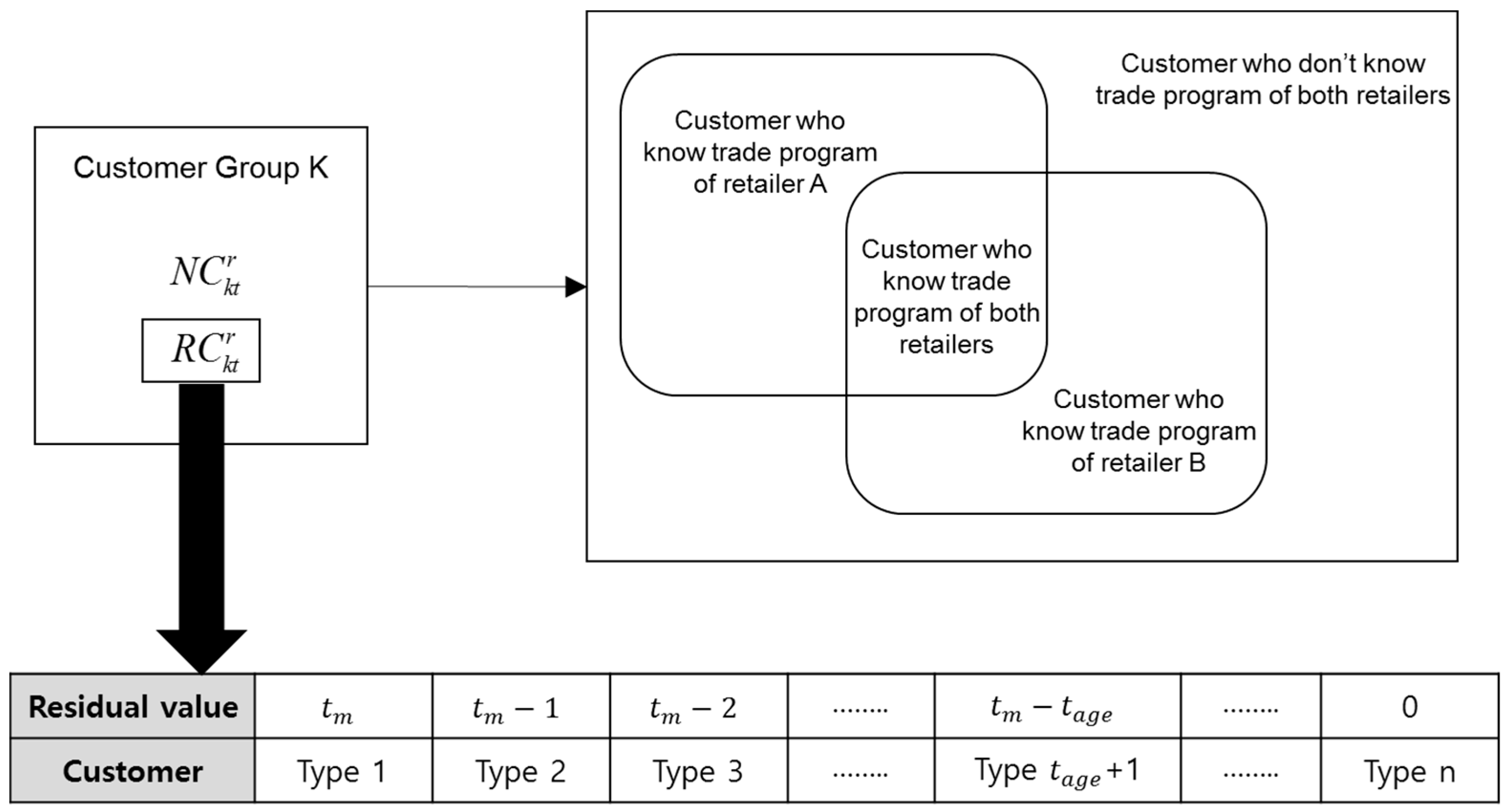
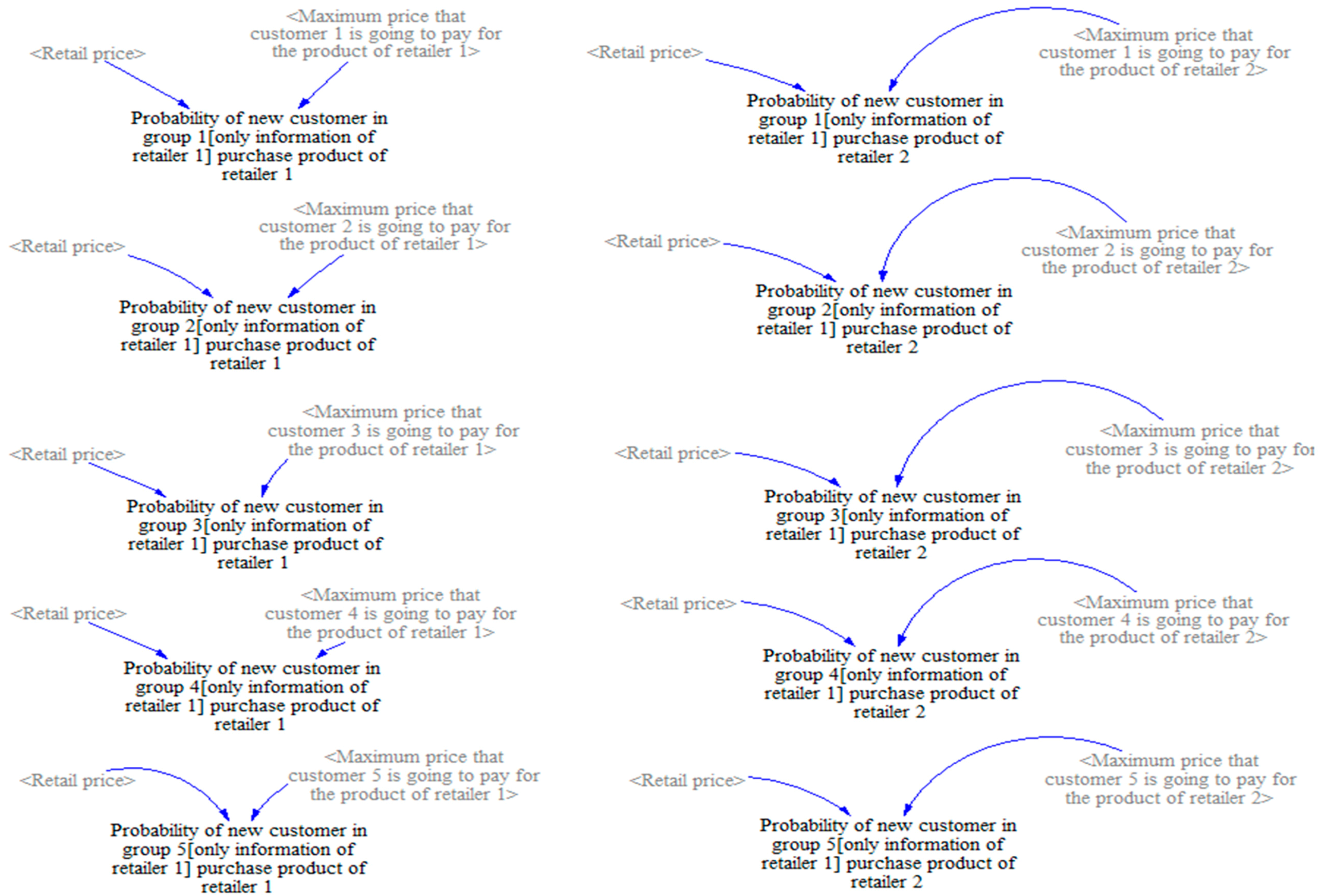
As shown in Figure 3, the current study assumes that new and replacement customers are classified into those who only know about the trade-in sale program offered by retailer A (), those who only know about that offered by retailer B (), those who know about the trade-in sale programs offered by both retailers (), and those who have no information about the programs of either retailer (). Formulas (2) through (5) represent the types of customers and, as they can be applied to new and replacement customers in the same manner, the displayed formulas only show the case for NCs.
Potential new customers generally make their purchase decisions solely on the basis of the price of the new product (). The current study assumes that both retailers sell their product at the same price. Replacement customers, however, make their purchase decisions based on the trade-in value and the remaining value of their used product. The remaining value is directly related to the amount of time passed during which the value of the initial product price declined [41,42]. The current study defines the maximum period of use for a product as . Thus, the remaining value for a customer who has used his or her old product for is . We assume that of customers follow a uniform distribution, where ; thus, replacement customers can be segmented further depending on their remaining value. This assumption supports the idea in the customer behavior literature that individual customers’ mental depreciation of a product is closely related to how long the product has been used [41].
3.3. Customer Purchase Behavior
The current study uses consumer surplus to consider the customers’ purchase decisions. In customer group k, each customer has a reservation price for the product. The reservation product for retailer r () is different for each customer group and for each customer within the group. The current study assumes that the reservation prices follow a uniform distribution, where . Here, represents the maximum price that the customer is willing to pay for the product. Assuming that the reservation price has a uniform distribution provides an easy framework in which to conduct the analysis and reflects the customer diversity extant in real markets. Furthermore, this pricing is a standard assumption used in most previous studies [43,44]. In addition, as the current study considers a market in which two retailers exist, different customer groups k can have different reservation prices for retailer A and retailer B. For example, customers located closer to retailer A have a higher reservation price for that retailer than does a customer living farther away. If there is no promotion for similar products, customers in general do not purchase the products from the retailer that is located farther away. Thus, the reservation price of a customer in group k for retailer r (retailer A or B) is defined as .
When making purchase decisions, new customers only consider the price of the product (), which leads to the expression of consumer surplus for retailers A and B in new customer in customer group k as shown in Formula (6).
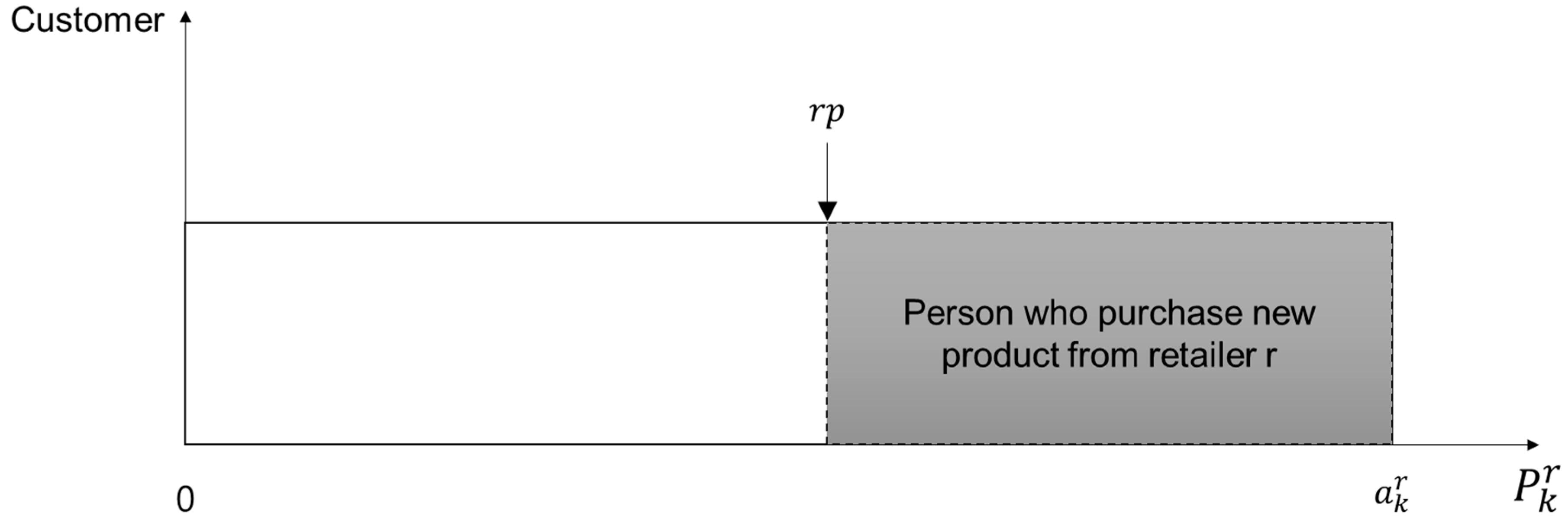
In addition, the possibility that a potential new customer randomly selected from will willingly purchase a new product from retailer A and B is describe in Formulas (7) and (8), respectively. To consider the effect of advertisements proffered by each retailer, this study distinguishes the probabilities of customers who have information about only one retailer and those who know about the sale programs of both retailers. Customers who only know about either retailer A or retailer B do not compare the two retailers’ products. Therefore, as shown in Figure 4, among customers who have information about only retailer A or retailer B, those with a higher reservation price than the selling price will ultimately buy the product. This study defines the purchase probability of customers in group k who only know about only retailer r as , as shown in Formula (7).
Among customers, those who have information about both companies will compare the products sold by retailers A and B before making a purchase decision. Therefore, as shown in Formula (7), the current study considers the share of customers purchasing from retailer A () and those purchasing from retailer B () relative to the maximum purchase probability of such customers to define the two groups of customers as and , respectively, as shown in Formula (8).
However, the potential replacement customers who own a product used for , in contrast to new customers, consider the trade-in value offered by the retailer () and the remaining value when purchasing a new product. In general, the higher the remaining value in the old product is, the lower the probability that a customer will purchase a new product. If a customer has a high affinity for the new product (his or her reservation price is high) and the retailer provides a high trade-in value for the used product, customers who own a product with a higher remaining value may purchase a new product. Thus, the consumer surplus of replacement customers can be expressed as in Formula (9).
As in the case of new customers, replacement customers can be categorized into those who only know about one retailer from its advertising campaigns and those who have information about both retailers. However, as replacement customers are further segmented by the length of time for which the old product was used, variable must also be considered. Customers with information about only one retailer are expressed as , as shown in Formula (10), and the remaining value and the trade-in value offered by the retailer in the formula are considered in calculating the purchase probability of new customers.
The goal of each retailer is to maximize its expected profit, which is the sum of the total profit that can be obtained from new customers in group k () and from replacement customers (). Based on the definitions provided above, Formulas (11) through (13) express the total profit that can be obtained from the two types of customers.
3.4. Simulation
The system dynamics model was built using Vensim Pro 5.92 [45], and used to measure how the investment decision making of two competing retailers and, accordingly, customer purchase behavior affect the profit changes of retailers in a CLSC. Figure 5 depicts the experimental procedure for simulation testing. We provide the detailed simulation model in Appendix A.
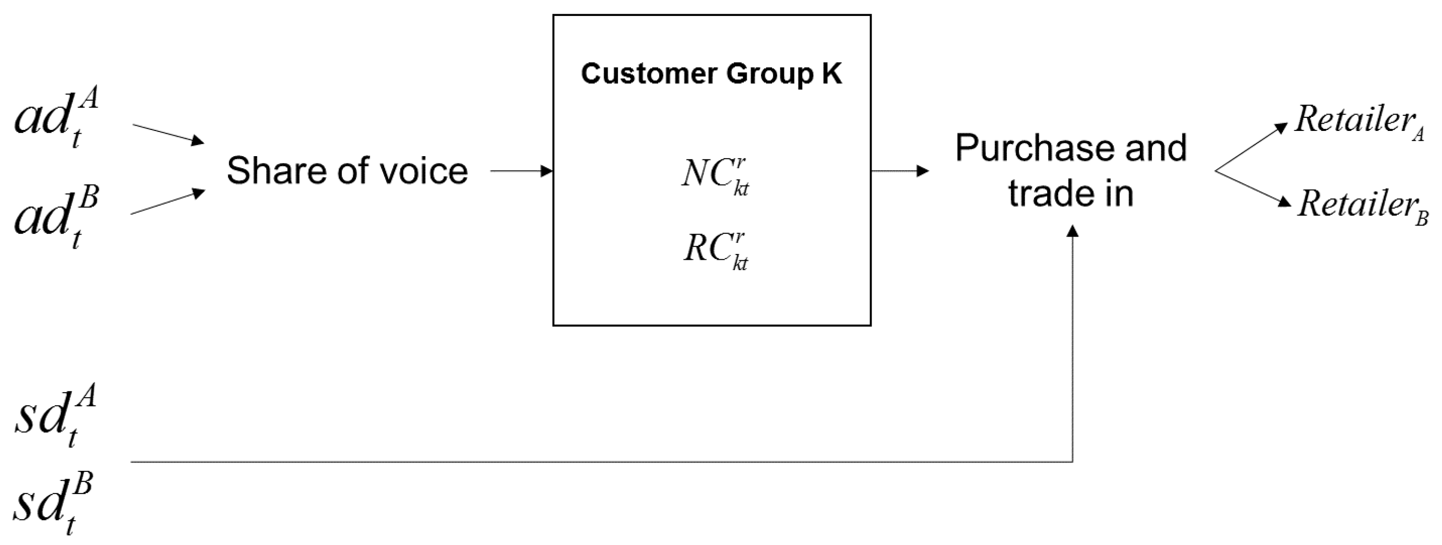
The time in the simulation model in the current study (a single time step) encompasses the comprehensive duopolistic competitive setting displayed in Figure 6. That is, at the initial point in time t, the two retailers (A and B) determine their investments in advertising and the trade-in allowance to induce product sales and trade-in sales in customer group k; the profits of each retailer from the purchase behaviors encouraged by such investments are calculated at the end of period t. In turn, during the initial phase of time period t + 1, the retailers determine new amounts of investment for their advertising and the trade-in allowance that reflect the investment-profit ratio in period t. Thus, the current model determines the advertising costs () and the trade-in allowance () of retailer r at the initial point of time period t, and this study emphasizes how the retailers’ profits change depending on the investment strategies suggested at the beginning.
4. Investment Strategy
“If you know your enemy and know yourself, you win 100 times out of 100 battles”—The Art of War, Sun Tzu.
In addition to academics, corporations have also have been engaged in research to win competitions, and analyzing and forecasting the competitors’ tactics, strategies, and capabilities laid the foundation laid the foundation for such endeavors. Day and Relistein [46] highlighted a failure to predict competitors’ movements and to identify potential interactions among competitors’ past activities as factors causing corporations to fail in complex competitive environments. In addition, Zajac and Bazerman [47] offered the critique that most decision-making processes are unable to infer competitors’ future actions. To win competitions, decision-makers must study the goals, strategies, strengths, and weaknesses of their competitors and understand the relationships among their past and present activities [48]. Furthermore, Montgomery et al. [49] argued that corporations should not stop at analyzing competitors but should further work to predict the latter’s future moves and generate a strategy in response and, in turn, analyze the competitors’ response to that strategy; they defined this cycle as strategic competitive reasoning. However, certain decision-makers ignore the behaviors of competitors. Leeflang and Witting [50] concluded that such companies believe that the successes and failures of corporate decision-making are the result of business capabilities and customer response, not of competitor activities. Furthermore, Jaworski and Wee [51] argued that significant amounts of effort and time are required to predict competitor businesses and their behavior, and extreme uncertainty in the results of a firm’s predictions may cause its strategy to fail. In sum, the literature notes that collecting the key information required to analyze and predict competitor behaviors is nearly impossible, and using relatively less-important information to analyze competitors can engender extremely uncertain results.
A study on the subject reveals that corporations face a choice between considering competitor strategies and using the results of their own past investments when drafting a competition plan. The present study considers four investment strategies with respect to advertising costs and trade-in allowance that can be employed by two retailers in a duopolistic competitive setting. The first option is to make investments based on information about their own past investments; the second is an imitative investment strategy that uses the competitor’s investment information; the third option is a strategy that uses both the competitor’s and the retailer’s own information; and the last strategy considers the future activities of the competitor. The following sections elaborate the four investment strategies.
Investment Strategy 1: Relying Solely on the Retailer’s Own Investment Information.
A company that relies solely on its own information determines its investment quantity in the present after comparing its past investment information () and changes to its profits due to its investment (). If the profit rate increased () when the trade-in allowance during cycle t − 1 was increased () compared to that of cycle t − 2, the company would identify the larger trade-in allowance as the cause of the profit growth and further increase the trade-in allowance in cycle t to continue the profit growth. However, such an increase in the trade-in allowance () may ultimately reduce the profit rate. In such a case, the company would determine that the increase in the trade-in value negatively impacted its profits and would decide to curb the trade-in allowance during cycle t. Formula (14) displays the current investment strategy with respect to the trade-in allowance based on the various results of past investment strategies. Because the same formula was applied to determine advertising investment, we do not repeat it.
This study assumes that all retailers participate in advertising and trade-in sale promotions at all times during cycle t, applies the maximum investment costs and in the same manner for both retailers, and assumes a minimum investment in the trade-in allowance and advertising of and for the two companies. We further assume that each retailer will add or subtract investments at the rate of to , which is the difference between the maximum investment quantity and the minimum investment quantity, when each retailer increases or decreases its investment quantity according to the profit rate associated with past investment information and profit rate changes. If a retailer maintains the amount of investment made in the previous cycle, the expression is . The investment in advertising costs uses the same mechanism as that for the trade-in allowance.
Investment Strategy 2: Imitative Investment (Aggressive or Defensive) Strategy Using Competitor Investment Information.
Here, the competitor () investment information used to determine the advertising costs and the trade-in allowance during cycle t includes the competitor’s profit rate () and investment quantity () during t − 1. If the retailer’s profit rate is higher than that of the competitor (), the retailer may judge that it is employing a better strategy than its competitor, meaning that it will invest the same amount as in the previous cycle. In contrast, if the competitor has a better profit rate (), the judgment would be that the competitor has a better investment strategy, which leads our retailer to imitate the competitor’s strategy to improve its profits. Thus, the retailer would add the difference between its own and the competitor’s investment in the previous cycle () to the amount of money it spent on investment in the previous cycle (). If the competitor made a larger investment in the previous cycle, our retailer would make additional investments, and if the competitor’s investment were smaller, the retailer’s investment would decrease. In addition, the retailer would make a judgment regarding whether its profits are exhibiting an upward () or downward trend () and employ an aggressive imitative strategy in the case of an upward trend (). As the investment cost is inversely related to profits, increasing investment during a downward trend in profits means that net profit might decrease; however, additional investment during an upward trend may attract more customers and therefore generate profit. Formula (15) displays this situation.
Investment Strategy 3: Investment Based on the Competitor and Retailer’s Own Investment Information.
This strategy combines the first and second investment strategies, whereby an imitative course of action is taken when the profit rate is lower than that of the competitor, and the retailer’s own past investment and profit information are used when its profit is higher than that of the competitor. The conditions are expressed in Formula (16).
Investment Strategy 4: Predicting Competitor Investment Information.
As noted in a previous section, using a competitor’s past actions to predict its future behavior and then establish the retailer’s own investment strategy is an effective method. Instead of using the investment quantity during cycle t − 1 in the imitative method in Strategy 2, we predict the investment quantity during cycle t using the moving average method. This method is employed because the competitor’s investment strategy during cycle t is unobservable; thus, an investment strategy is established by predicting the competitor’s future investment quantity. Formula (17) elaborates this approach.
5. Numerical Study
5.1. Setting the Experimental Parameters
The goal of the current study is to understand the effect of the above four investment strategies on the profits of retailers A and B. Table 1 displays the values of the basic parameters required to conduct this experiment.
5.2. Experimental Scenario
The key criterion that distinguishes the four investment strategies suggested by the current study is whether the retailers consider their competitor’s investment strategy in establishing their own plans. In a duopolistic competitive setting, we consider the following three scenarios: first, neither retailer considers the competitor’s investment information; second, one retailer considers the competitor’s investment information, while the other does not; and third, both retailers consider the competitor’s investment strategy. Table 2 shows the experimental plan in the three scenarios.
5.3. Experimental Results
Table 3 summarizes the average profit, the sales amount, the investment cost, and the return on investment (ROI) derived from the experiments for each scenario.
Scenarios 1 to 2.3 report the results of each investment strategy when retailer B has a low investment amount and, when retailer A has a high initial investment amount, determines its investment level by considering its own profit information. When developing an investment strategy that considers its own profit changes and investment trends without considering the competitor’s profits and investment information (scenario 1), the retailer that invests more in advertising and trade-in sales maintains higher returns.
As shown in the results for scenario 1, the average profit of retailer A is 13.8% higher than that of retailer B. This is because each retailer believes that changes in its own profits result from the relationship between past investment patterns and changes in profit. For retailer B, the ROI of scenario 1 showed the best results. However, the total profit of retailer B is the lowest of the scenarios considered. The reason that the ROI is favorable is because it minimizes the investment level. Because retailer B, which has a lower investment, could not plan to aggressively determine the size of its investment without considering its competitor, it will maintain a low level of investment if it continues using investment strategy (1).
Next, the changes in retailer B’s investment level and profits were analyzed in the case in which retailer B decides to consider the investment information of retailer A. If the profit of retailer B is lower than that of retailer A, it will follow the investment amount of retailer A; when retailer B attains higher returns, the current investment amount is considered optimal and is thus maintained. In Table 3, the average investment in the advertising and trade-in sales by retailer B has increased by approximately 13.4% and 18.3%, respectively, which is more than the corresponding results from scenario 1; the average profit in this scenario improved by approximately 9.6%.
Although scenario 2.1 improved the average profits of retailer B relative to scenario 1, the ROI deteriorated. It appears that retailer B has decided to make excessive investments to gain more customers at a lower profit point than retailer A.
Scenario 2.2 showed the best result for the total profit of retailer B. Here, retailer B follows the investment amount of retailer A when retailer B’s profit is lower. As retailer B’s profits are higher than those of its competitor, it determines its own investment strategy by considering only the relationship between its investment level and profits. This strategy leads to higher investment in advertising (an approximately 26.5% increase) and trade-in sales (an approximately 7.5% increase) for retailer B relative to scenario 1. Based on these findings, the average profit is improved by approximately 15.3% compared to scenario 1. The results of scenario 2.2 produce the highest average profit but the worst ROI for retailer B among the scenarios considered. These results are due to the excessive investments made by retailer B relative to those of retailer A.
In scenario 2.3, when retailer B has a lower profit than retailer A, B determines its own investment by analyzing the investment trends of retailer A in the past few periods, instead of following A’s investment level as in scenario 2.2. In this scenario, the amounts invested by retailer B in adverting and trade-in sales decreased by approximately 4.8% and 3.5%, respectively, relative to scenario 2.1. In terms of its average profit and ROI, scenario 2.3 is the most reliable investment strategy available for retailer B.
In this study, we also perform ANOVA analysis to ensure that there is a significant difference in the mean ROI values across scenarios, and the Fisher method was used for ex post examination. Table 4 summarizes the results of scenarios 1 and 2.1 to 2.3. The F-value for the mean ROI of the four scenarios was 1410.99 and the p-value was significant at the 0.05 level. Therefore, the mean ROI of all scenarios is not equal to that of the four scenarios because the differences in the ROI average do not include 0, as shown in Figure 7. Scenario 1 showed the best performance.
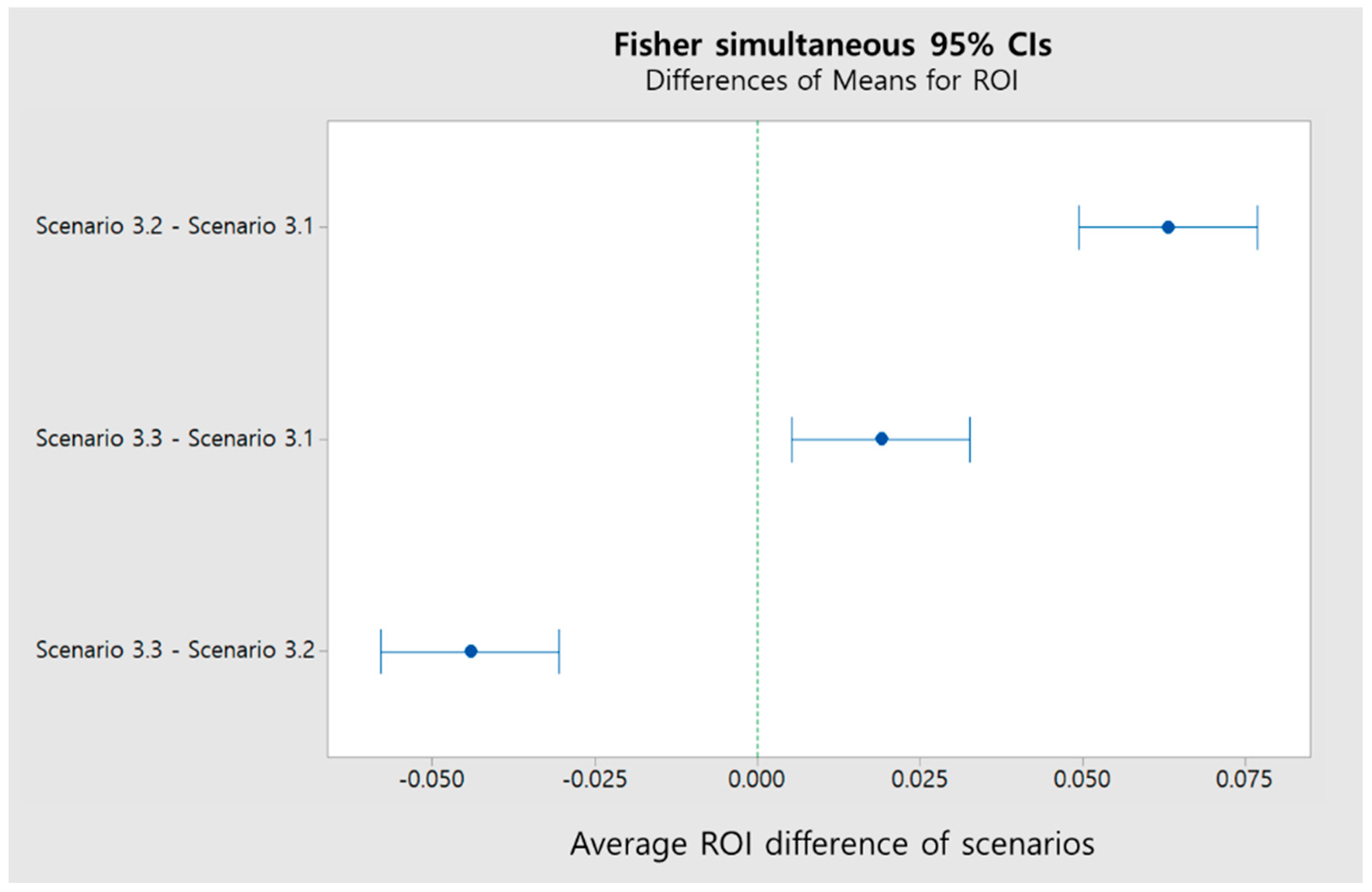
The results from scenarios 1 and 2.1 to 2.3 above compared the performance of the investment strategies of the competitor when a retailer with a higher investment determines its own investment level when only considering its own profits. However, it is more realistic for both competitors to consider their own investment levels when considering the opposite party’s investment strategies. Thus, here, we analyze the change in profits and ROI for both retailers through scenarios 3.1 to 3.3. Overall, both retailers showed signs of excessive competition, in the sense that they made higher investments than previously. As shown in Table 5, these results entail higher investment in advertising and trade-in sales for both retailers relative to scenarios 1 and 2.1 to 2.3 and thus lower average profits.
In scenario 3.3, by considering the investment trends of retailer A, retailer B decided its own investment amount and was able to reduce unnecessary investment. This result entailed better profits and ROI than in scenario 3.1.
In the results of scenario 3.2, initially, the overheated competition between the two competitors is apparent. However, after retailer B, which has a relatively low initial investment, amount obtains a higher profit than retailer A, retailer B did not engage in excessive investment because it considered the changes in profits compared to its own investment amount. By preventing excessive investment arising from overheated competition when retailer B becomes more profitable, retailer B implemented a strategy to maintain higher profits through reduced investment costs. This strategy contributes to the improvement in the average profit and ROI of retailer B compared to those in scenarios 3.1 and 3.3.
6. Conclusions
Existing CLSC have focused on ways to increase the return amount from customers who have used products. We noted that retailers have the opportunity to sell new products by securing the return amount. We are interested in investment strategies of retailers to attract customers who wish to benefit from purchasing new products by returning used products. These investment strategies are determined by the advertising expenditure for spreading customers’ awareness and the trade-in allowances for increasing sales promotion of new products. They are affected by whether or not a retailer considers the competitor’s investment information. The selection and application of the effective investment strategy of a retailer changes the behavior of customer purchases and ultimately contributes to improve its own profit.
The experiment results have provided if a retailer did not consider competitor’s investment information when establishing investment strategy, even though the market size decreased slightly, the intensity of the competition decreased and eventually increased its own ROI. On the other hand, when a retailer consider competitor’s investment information, the high investment cost caused by the overheated competition will result in decreased ROI, despite the growing market size.
From this point of view, if retailer wants to increase the average ROI, it is effective to establish an investment strategy without considering the investment information from competitors. However, the establishment of investment strategy reflecting competitor’s investment information has the advantage of boosting the market size by inducing higher investment costs from two competing retailers. Increasing of market size will be beneficial to retailers that compete in durable product market, since they want potential replacement customers to make loyal customers who have both an attitudinal and behavioral tendency to favor one brand over all others. Securing a customer’s loyalty can lead customer to repurchase new products.
Our work provides theoretical contributions by linking the marketing factors such as consumer’s surplus, trade-in allowances, advertising diffusion and the competitive market in the traditional CLSC while most of CLSC studies have focused on operational approaches and coordinative strategies. We also offer a practical application by analyzing how investment strategies of each retailer affect purchasing behavior of customers who have different consumer surplus and residual value for used products in the competing market with two retailers. However, we point out the limitations of our study and suggest a few possible extensions that pertain to our model. Our study targeted the competitive market with only two homogenous retailers and assumed that retailers use a locked investment strategy during simulation periods for the simplification. In real market, however, multiple heterogeneous retailers who differ the market share and handle goods with different quality compete. In according to the market status and their position of market, they also often alter their investment strategies over time. Our model did not represent these phenomena due to the complexity of model. However, we expect future works using advanced simulation modeling technique or new approaches facilitate to overcome the drawbacks of our research.
Acknowledgments
The present research has been conducted by the Research Grant of Kwangwoon University in 2016. This work was supported by the Ministry of Education of Republic of Korea and the National Research Foundation of Korea (NRF-2015S1A5A2A01010855).
Author Contributions
Sungwook Yoon has developed the model and performed the experiments. He also wrote the experimental section of the paper. Sukjae Jeong has created the overall idea and the basic outline of the paper.
Conflicts of Interest
The authors declare no conflict of interest.
Appendix A. Simulation Modeling
Figure A1.
Model part 1: Retailer’s investment decision for the subsidy and the advertising in period t.
Figure A1.
Model part 1: Retailer’s investment decision for the subsidy and the advertising in period t.
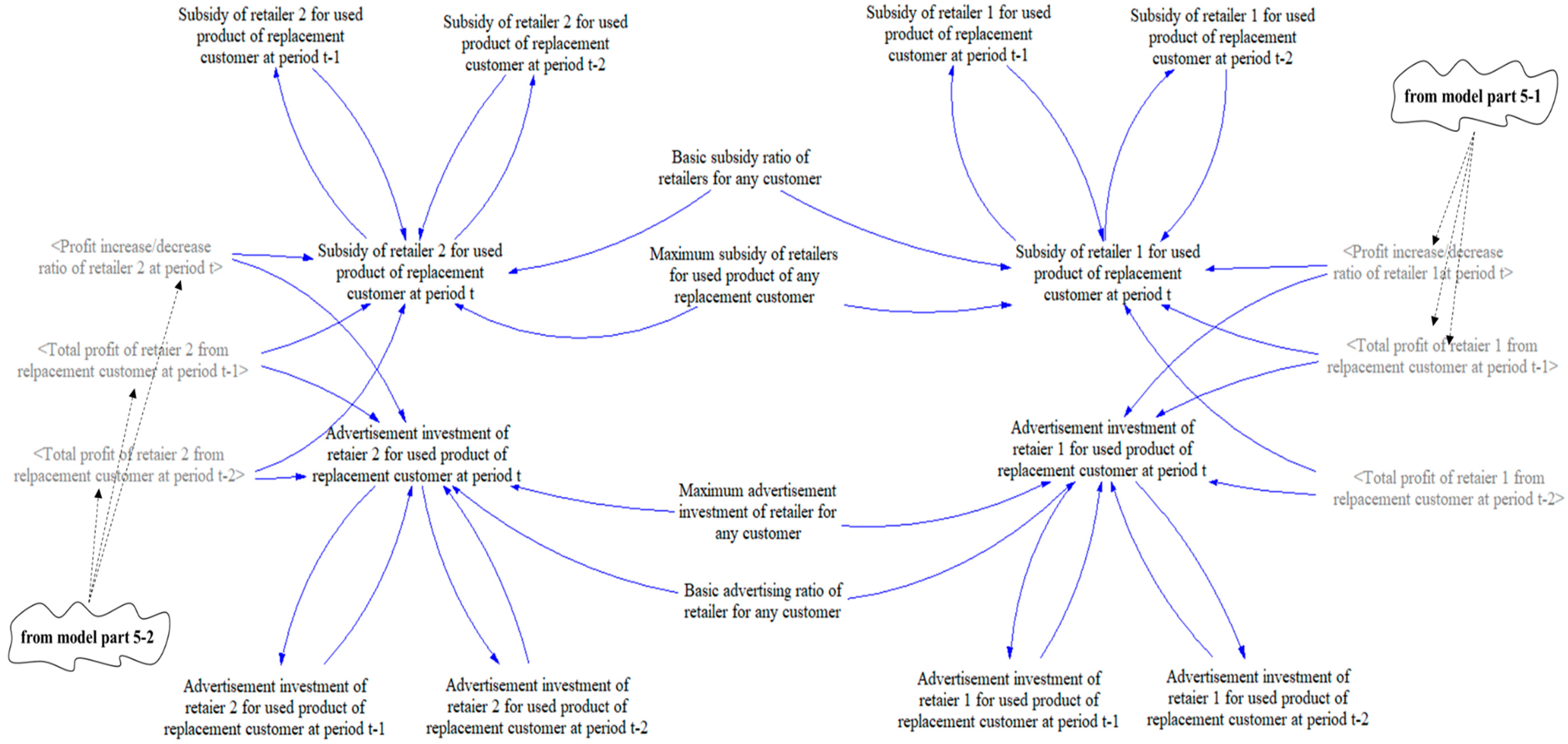
Figure A2.
Model part 2: Customers classification according to whether customers have information about single retailer or both retailers.
Figure A2.
Model part 2: Customers classification according to whether customers have information about single retailer or both retailers.
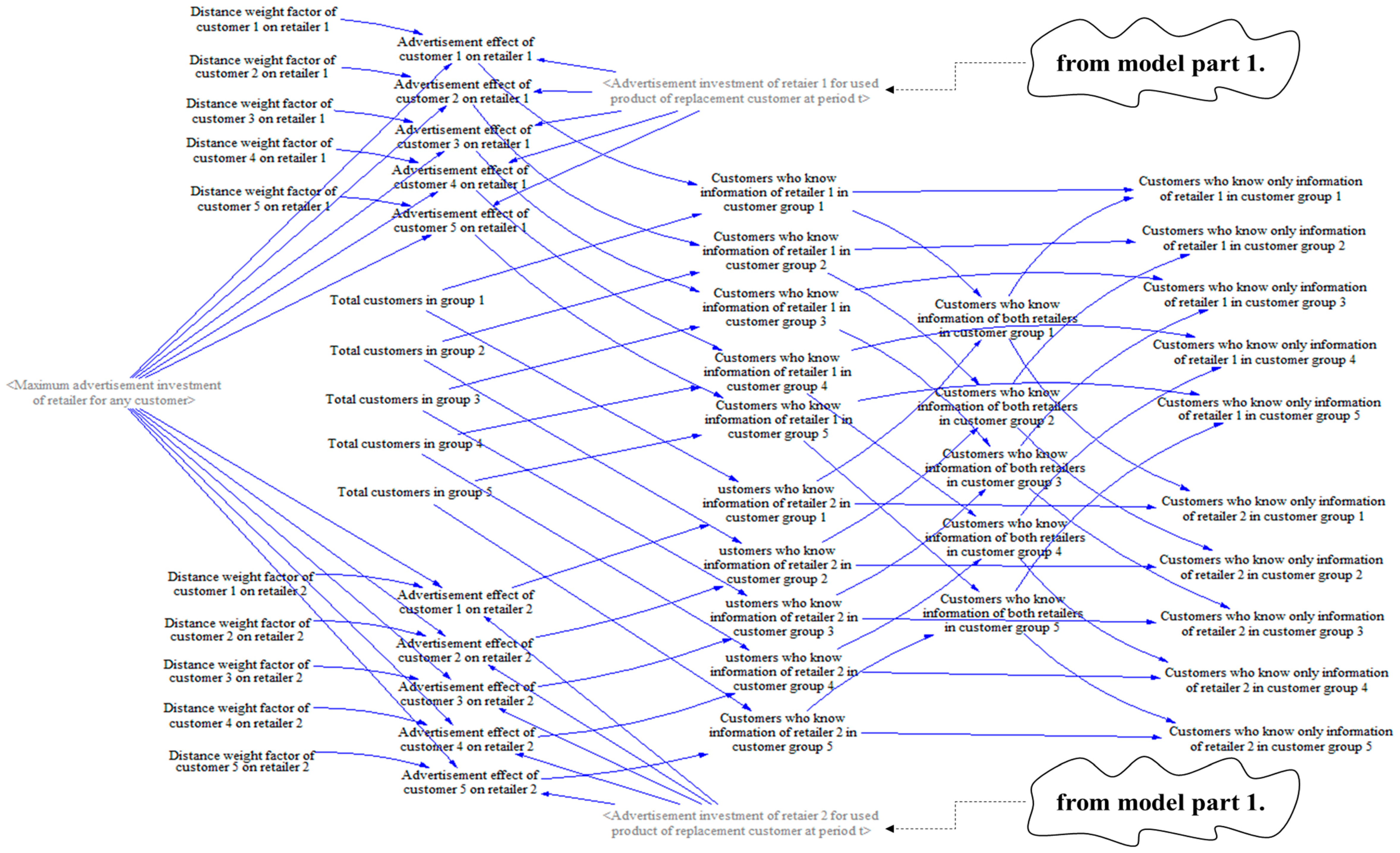
Figure A3.
Model part 3-1: Probability that replacement customer who have information about one retailer purchases retailer r’s product.
Figure A3.
Model part 3-1: Probability that replacement customer who have information about one retailer purchases retailer r’s product.
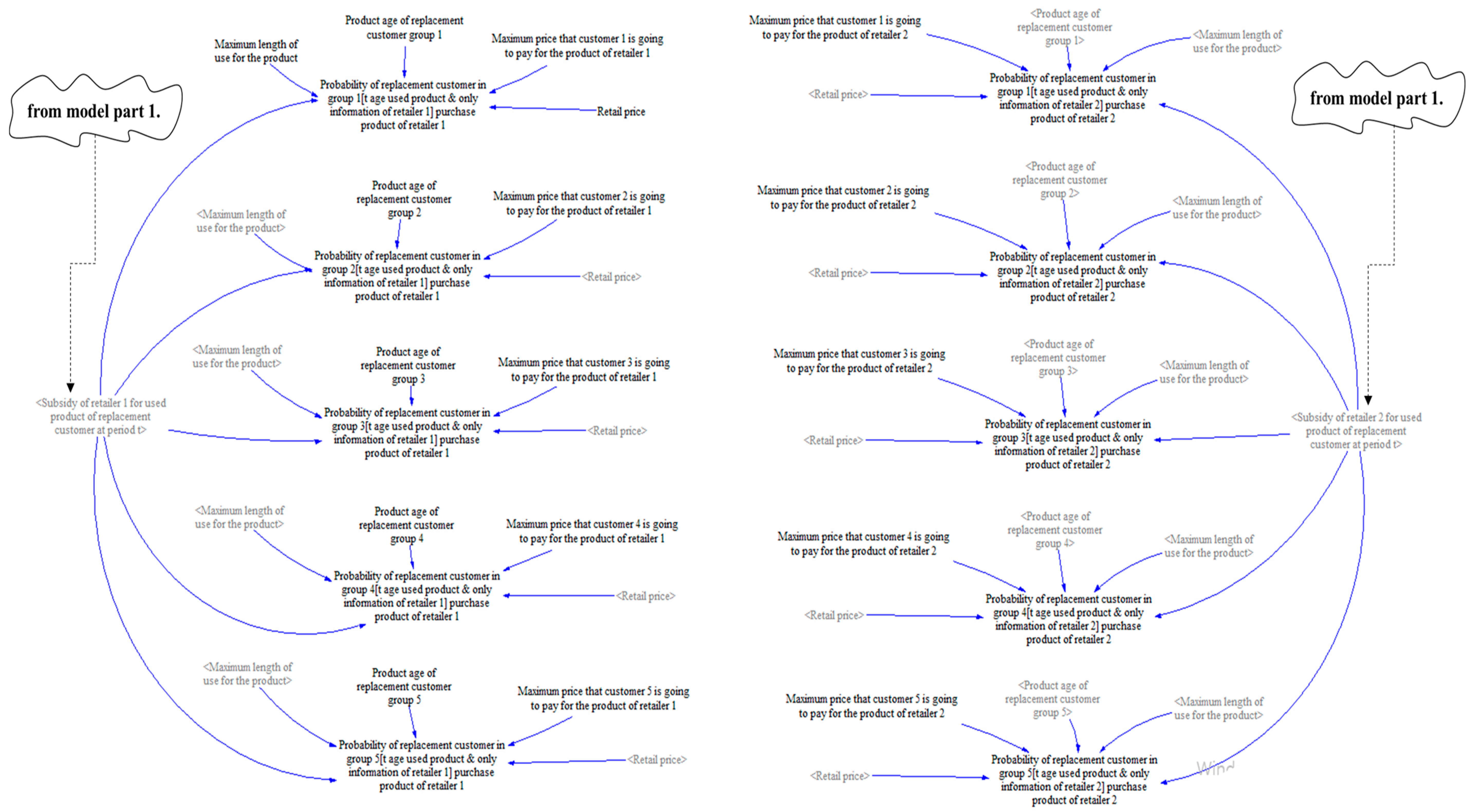
Figure A4.
Model part 3-2: Probability that replacement customer who have information about both retailers purchases retailer r’s product.
Figure A4.
Model part 3-2: Probability that replacement customer who have information about both retailers purchases retailer r’s product.
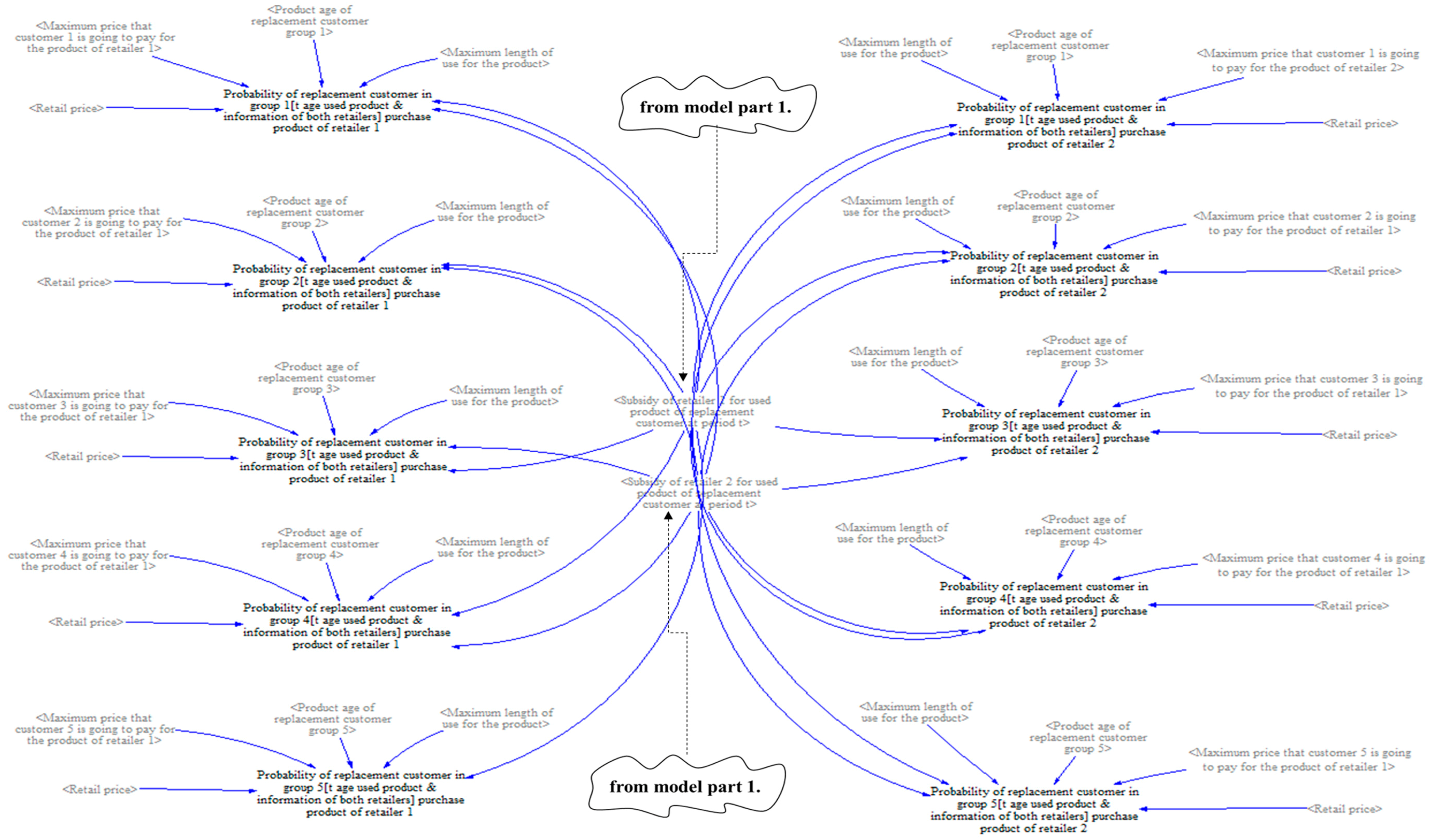
Figure A5.
Model part 3-3: Probability that new customer who have information about one retailer purchases retailer r’s product.
Figure A5.
Model part 3-3: Probability that new customer who have information about one retailer purchases retailer r’s product.

Figure A6.
Model part 3-4: Probability that new customer who have information about both retailers purchases retailer r’s product.
Figure A6.
Model part 3-4: Probability that new customer who have information about both retailers purchases retailer r’s product.
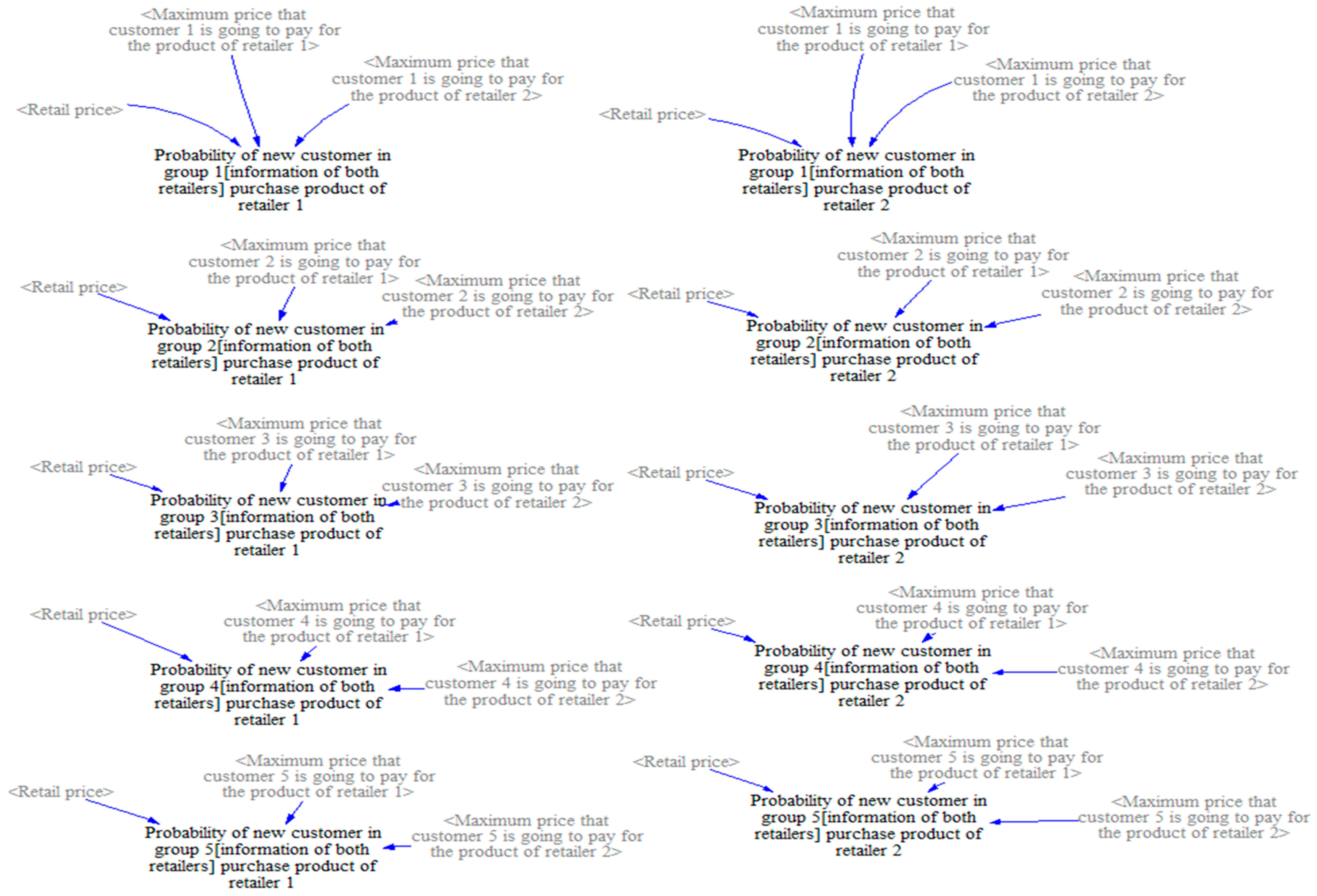
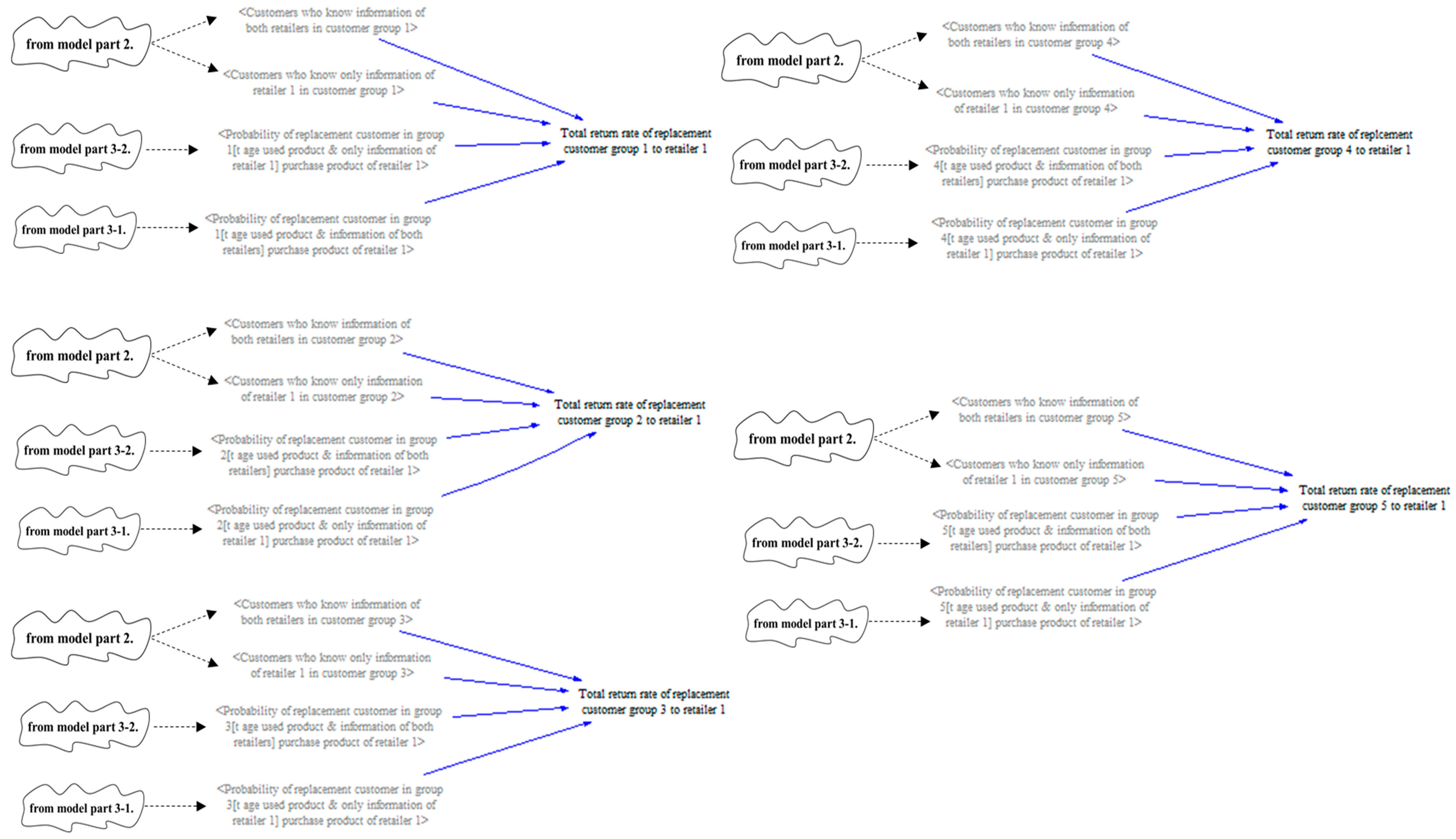
Figure A7.
Model part 4-1: Total amount retuned to retailer 1 from replacement customer by each group.
Figure A7.
Model part 4-1: Total amount retuned to retailer 1 from replacement customer by each group.

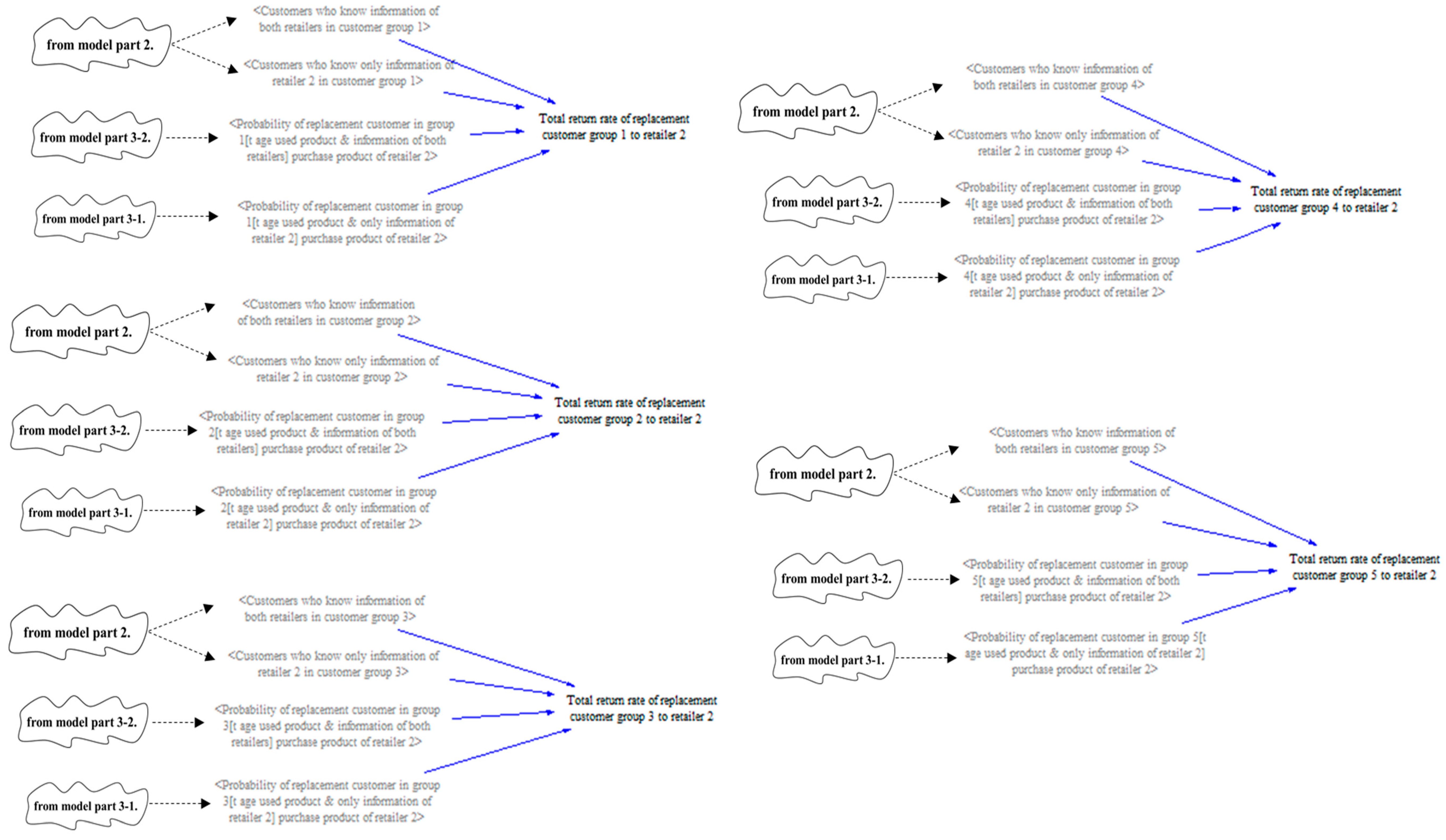
Figure A8.
Model part 4-2: Total amount retuned to retailer 2 from replacement customer by each group.
Figure A8.
Model part 4-2: Total amount retuned to retailer 2 from replacement customer by each group.

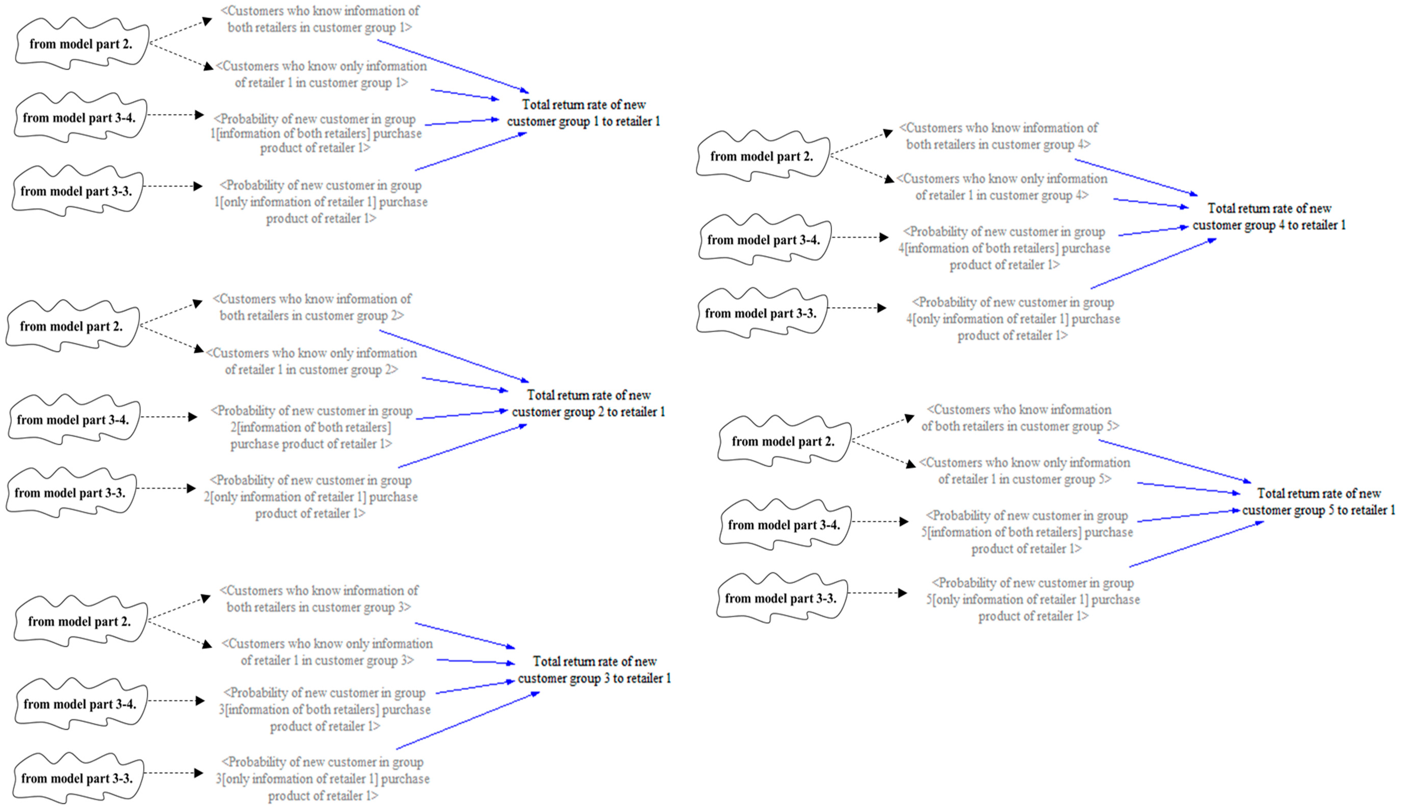
Figure A9.
Model part 4-3: Total amount retuned to retailer 1 from new customer by each group.

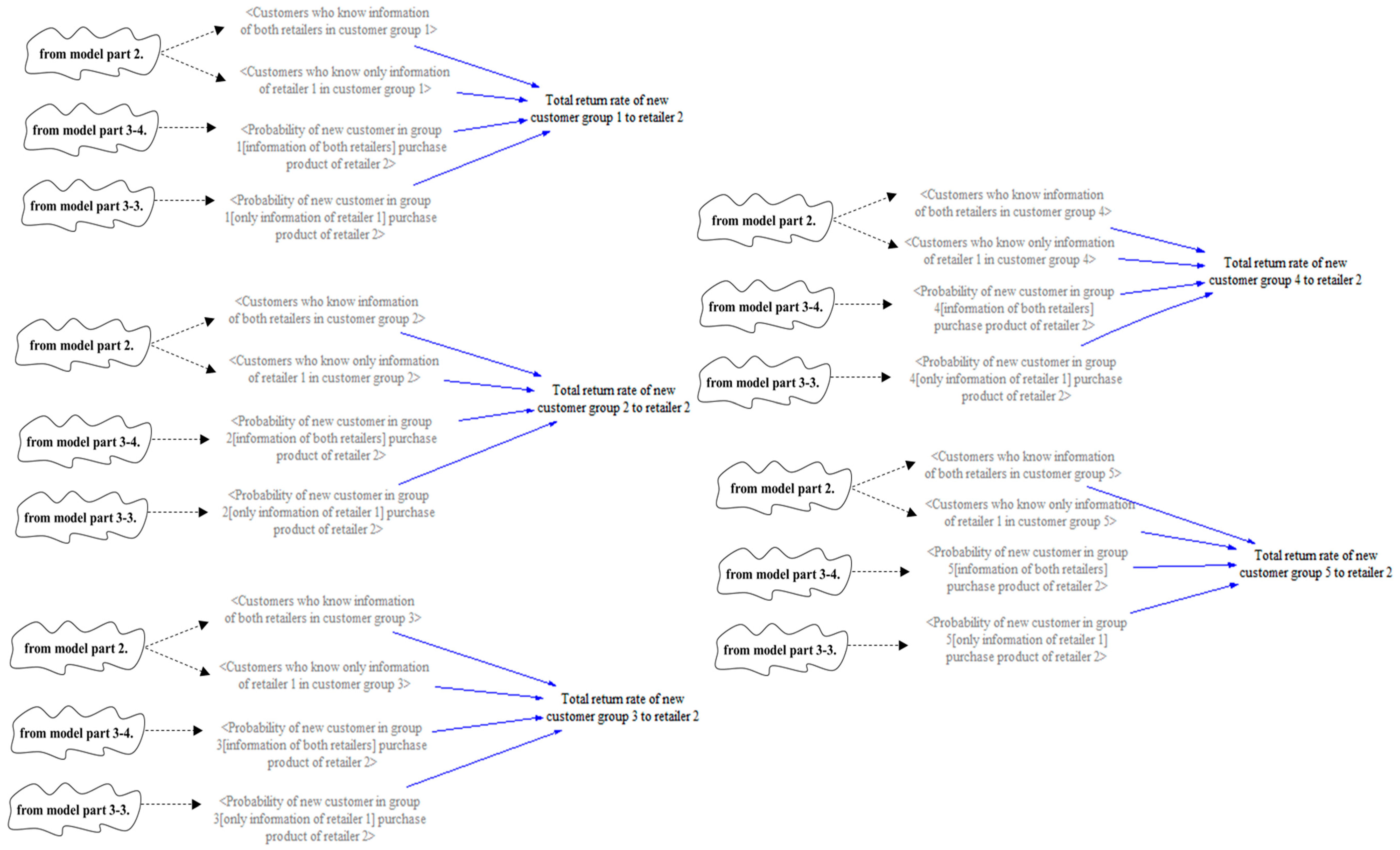
Figure A10.
Model part 4-4: Total amount retuned to retailer 2 from new customer by each group.

Figure A11.
Model part 5-1: Total profit of retailer 1 in period t.
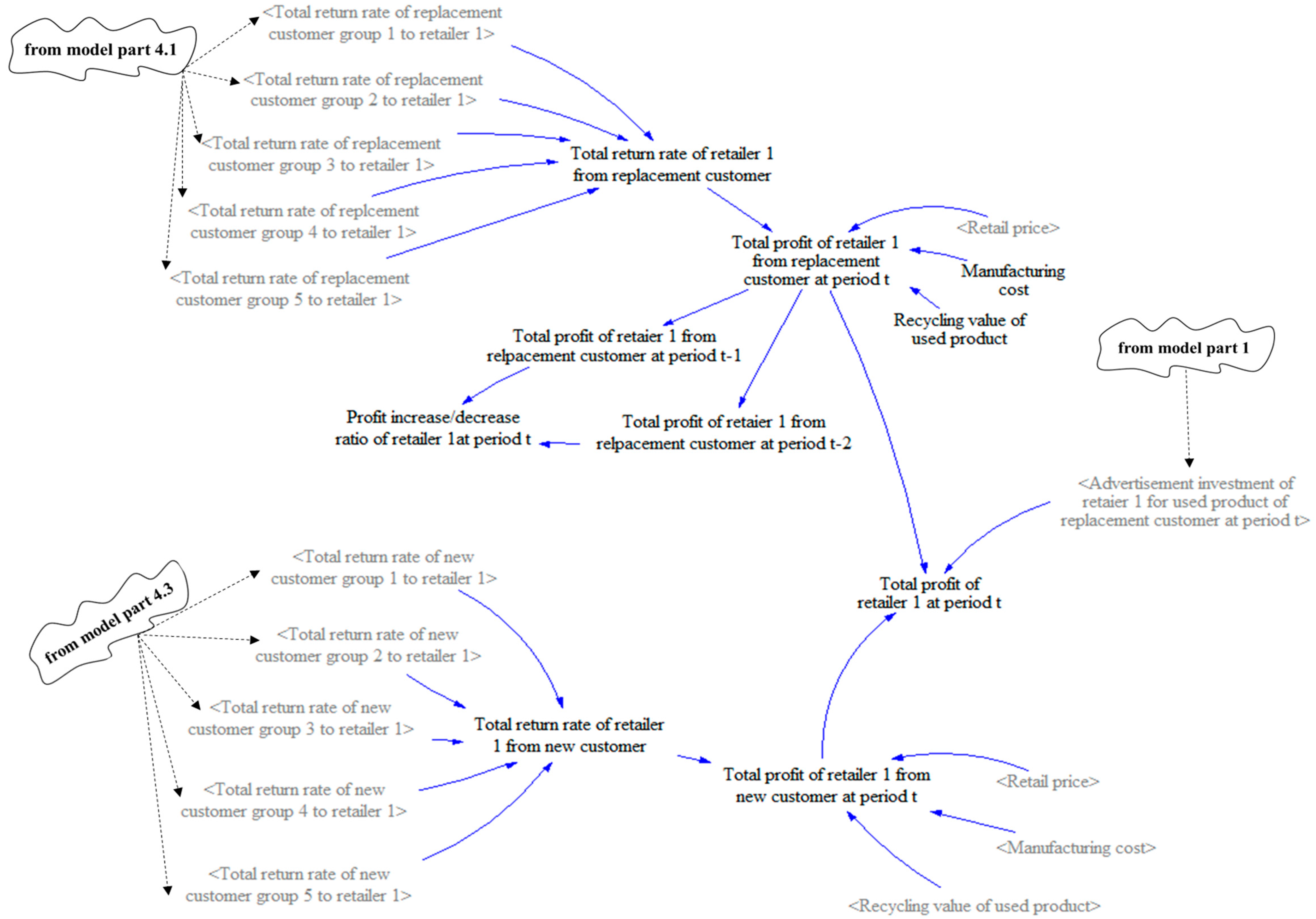
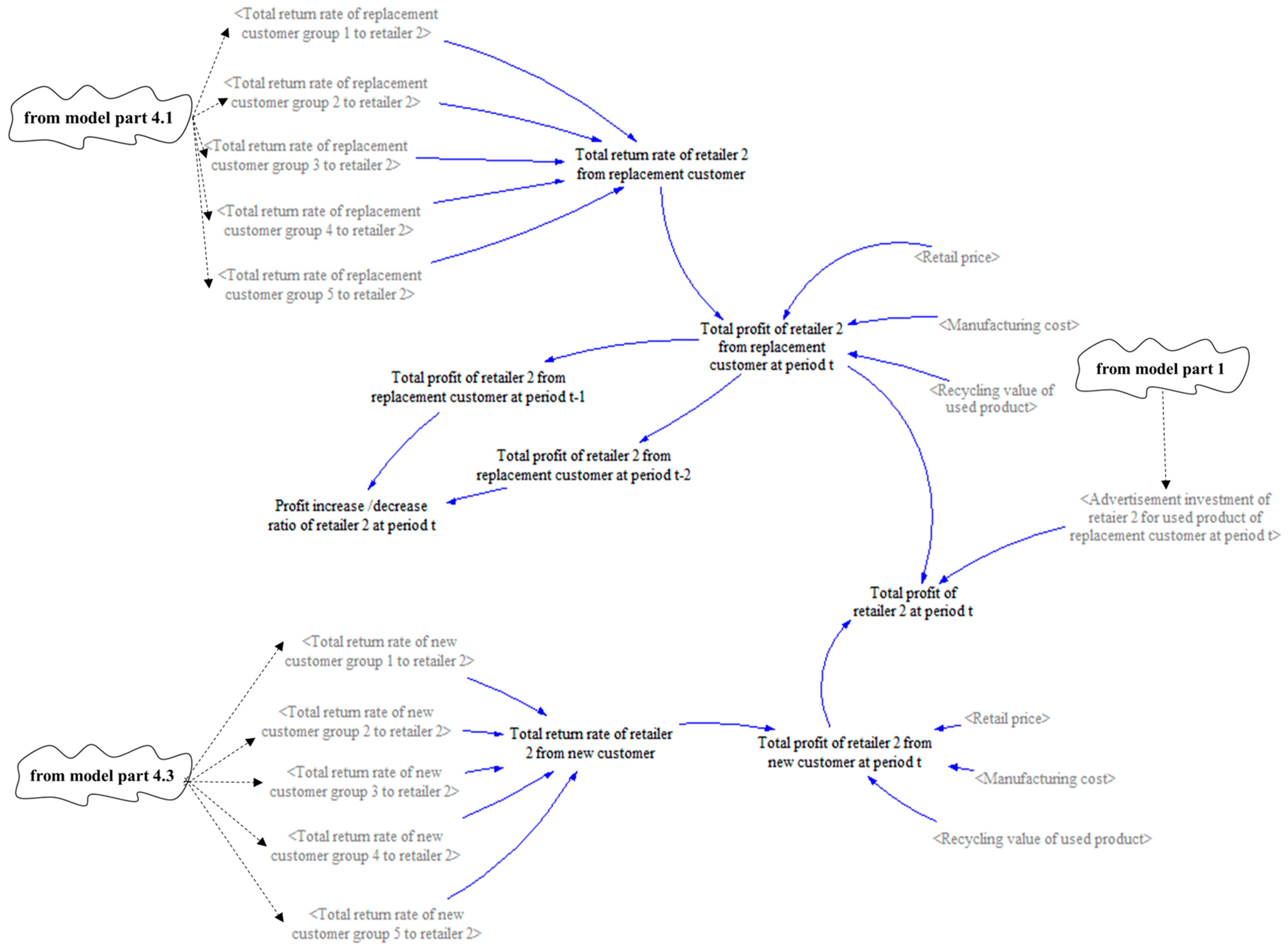
Figure A12.
Model part 5-2: Total profit of retailer 2 in period t.

References
- Kotler, P.; Saliba, S.; Wrenn, B. Marketing Management: Analysis, Planning, and Control: Instructor’s Manual; Prentice-Hall: Upper Saddle River, NJ, USA, 1991. [Google Scholar]
- Fishbein, B.K.; McGarry, L.S.; Dillon, P.S. Leasing: A Step toward Producer Responsibility. Available online: http://dx.doi.org/10.1162/10881980160084079 (accessed on 22 September 2017).
- Klausner, M.; Hendrickson, C.T. Reverse-logistics strategy for product take-back. Interfaces 2000, 30, 156–165. [Google Scholar] [CrossRef]
- WasteWise Update. Remanufactured Products: Good as New. United States Environmental Protection Agency, Solid Wasteand Emergency Response. EPA530-N-97-002; 1997. Available online: http://pasmand.tehran.ir/Portals/0/Document/maghale/0-magazin/wwupda6.pdf (accessed on 22 September 2017).
- Grosvold, J.; Hoejmose, S.U.; Roehrich, J.K. Squaring the circle: Management, measurement and performance of sustainability in supply chains. Supply Chain Manag. 2014, 19, 292–305. [Google Scholar] [CrossRef]
- Qingmei, T.; Dongyi, W. Managerial Power and Firm Value: Based on the Perspective of Product Market Competition. J. Manag. 2014, 3, 1–13. [Google Scholar]
- Ray, S.; Boyaci, T.; Aras, N. Optimal prices and trade-in rebates for durable, remanufacturable products. Manuf. Serv. Oper. Manag. 2005, 7, 208–228. [Google Scholar] [CrossRef]
- Shi, T.; Gu, W.; Chhajed, D.; Petruzzi, N.C. Effects of remanufacturable product design on market segmentation and the environment. Decis. Sci. 2016, 47, 298–332. [Google Scholar] [CrossRef]
- Rao, R.S.; Narasimhan, O.; John, G. Understanding the role of trade-ins in durable goods markets: Theory and evidence. Market. Sci. 2009, 28, 950–967. [Google Scholar] [CrossRef]
- Zhu, X.; Wang, M.; Chen, G.; Chen, X. The effect of implementing trade-in strategy on duopoly competition. Eur. J. Oper. Res. 2016, 248, 856–868. [Google Scholar] [CrossRef]
- Horsky, D.; Simon, L.S. Advertising and the diffusion of new products. Market. Sci. 1983, 2, 1–17. [Google Scholar] [CrossRef]
- Manickam, S.A. Do advertising tools create awareness, provide information, and enhance knowledge? An exploratory study. J. Promot. Manag. 2014, 20, 291–310. [Google Scholar] [CrossRef]
- Savaskan, R.C.; van Wassenhove, L.N. Reverse Channel Design: The Case of Competing Retailers. Manag. Sci. 2006, 52, 1–14. [Google Scholar] [CrossRef]
- De Giovanni, P.; Zaccour, G. A two-period game of a closed-loop supply chain. Eur. J. Oper. Res. 2014, 232, 22–40. [Google Scholar] [CrossRef]
- De Giovanni, P.; Reddy, P.V.; Zaccour, G. Incentive strategies for an optimal recovery program in a closed-loop supply chain. Eur. J. Oper. Res. 2016, 249, 605–617. [Google Scholar] [CrossRef]
- Van der Laan, E.; Salomon, M.; Dekker, R.; Van Wassenhove, L. Inventory Control in Hybrid Systems with Remanufacturing. Manag. Sci. 1999, 45, 733–747. [Google Scholar] [CrossRef]
- Toktay, L.B.; Wein, L.M.; Zenios, S.A. Inventory Management of Remanufacturable Products. Manag. Sci. 2000, 46, 1412–1426. [Google Scholar] [CrossRef]
- Fleischmann, M.; Beullens, P.; Bloemhof-Ruwaard, J.M.; van Wassenhove, L.N. The Impact of Product Recovery on Logistics Network Design. Prod. Oper. Manag. 2001, 10, 156–173. [Google Scholar] [CrossRef]
- Bhattacharya, S.; van Wassenhove, L.N.; Guide, V.D.R., Jr. Optimal Order Quantities with Remanufacturing Across New Product Generations. Prod. Oper. Manag. 2006, 15, 421–431. [Google Scholar] [CrossRef]
- Guide, V.D.R., Jr.; Jayaraman, V.; Linton, J.D. Building contingency planning for closed-loop supply chains with product recovery. J. Oper. Manag. 2003, 21, 259–279. [Google Scholar] [CrossRef]
- Savaskan, R.C.; Bhattacharya, S.; van Wassenhove, L.N. Closed-Loop Supply Chain Models with Product Remanufacturing. Manag. Sci. 2004, 50, 239–252. [Google Scholar] [CrossRef]
- Guide, V.D.R., Jr.; Souza, G.C.; van Wassenhove, L.N.; Blackburn, J.D. Time Value of Commercial Product Returns. Manag. Sci. 2006, 52, 1200–1214. [Google Scholar] [CrossRef]
- Geyer, R.; van Wassenhove, L.N.; Atasu, A. The Economics of Remanufacturing under Limited Component Durability and Finite Product Life Cycles. Manag. Sci. 2007, 1, 88–100. [Google Scholar] [CrossRef]
- Zikopoulos, C.; Tagaras, G. On the attractiveness of sorting before disassembly in remanufacturing. IIE Trans. 2008, 40, 313–323. [Google Scholar] [CrossRef]
- Sherafati, M.; Bashiri, M. Closed loop supply chain network design with fuzzy tactical decisions. J. Ind. Eng. Int. 2016, 12, 255–269. [Google Scholar] [CrossRef]
- Mafakheri, F.; Nasiri, F. Revenue sharing coordination in reverse logistics. J. Clean. Prod. 2013, 59, 185–196. [Google Scholar] [CrossRef]
- Govindan, K.; Popiuc, M.N. Reverse supply chain coordination by revenue sharing contract: A case for the personal computers industry. Eur. J. Oper. Res. 2014, 233, 326–336. [Google Scholar] [CrossRef]
- Li, S.; Zhu, Z.; Huang, L. Supply chain coordination and decision making under consignment contract with revenue sharing. Int. J. Prod. Econ. 2009, 120, 88–99. [Google Scholar] [CrossRef]
- Yoon, S.W.; Jeong, S.J. Implementing Coordinative Contracts between Manufacturer and Retailer in a Reverse Supply Chain. Sustainability 2016, 8, 913. [Google Scholar] [CrossRef]
- Koçaş, C.; Bohlmann, J.D. Segmented switchers and retailer pricing strategies. J. Market. 2008, 72, 124–142. [Google Scholar] [CrossRef] [Green Version]
- Yin, R.; Tang, C.S. Optimal Temporal Customer Purchasing Decisions under Trade-In Programs with Up-Front Fees. Decis. Sci. 2014, 45, 373–400. [Google Scholar] [CrossRef]
- Rajiv, S.; Dutta, S.; Dhar, S.K. Asymmetric store positioning and promotional advertising strategies: Theory and evidence. Market. Sci. 2002, 21, 74–96. [Google Scholar] [CrossRef]
- Joshi, Y.V.; Reibstein, D.J.; Zhang, Z.J. Turf Wars: Product Line Strategies in Competitive Markets. Market. Sci. 2015, 35, 128–141. [Google Scholar] [CrossRef]
- Delre, S.A.; Panico, C.; Wierenga, B. Competitive strategies in the motion picture industry: An ABM to study investment decisions. Int. J. Res. Market. 2017, 34, 69–99. [Google Scholar] [CrossRef]
- Roehrich, J.K.; Roehrich, J.K.; Hoejmose, S.U.; Overland, V. Driving green supply chain management performance through supplier selection and value internalization: A self-determination theory perspective. Int. J. Oper. Prod. Manag. 2017, 37, 489–509. [Google Scholar] [CrossRef]
- Walker, H.; Preuss, L. Fostering sustainability through sourcing from small businesses: Public sector perspectives. J. Clean. Prod. 2008, 16, 1600–1609. [Google Scholar] [CrossRef]
- Hoejmose, S.U.; Roehrich, J.K.; Grosvold, J. Is doing more doing better? The relationship between responsible supply chain management and corporate reputation. Ind. Market. Manag. 2014, 43, 77–90. [Google Scholar] [CrossRef]
- Clifford Defee, C.; Esper, T.; Mollenkopf, D. Leveraging closed-loop orientation and leadership for environmental sustainability. Supply Chain Manag. 2009, 14, 87–98. [Google Scholar] [CrossRef]
- Preuss, L. Addressing sustainable development through public procurement: The case of local government. Supply Chain Manag. 2009, 14, 213–223. [Google Scholar] [CrossRef]
- Kramer, M.R.; Porter, M.E. Strategy and society: The link between competitive advantage and corporate social responsibility. Harv. Bus. Rev. 2006, 84, 78–92. [Google Scholar]
- Heath, C.; Fennema, M.G. Mental depreciation and marginal decision making. Organ. Behav. Hum. Decis. Process. 1996, 68, 95–108. [Google Scholar] [CrossRef] [PubMed]
- Okada, E.M. Trade-ins, mental accounting, and product replacement decisions. J. Consum. Res. 2001, 27, 433–446. [Google Scholar] [CrossRef]
- Van Ackere, A.; Reyniers, D.J. Trade-ins and introductory offers in a monopoly. RAND J. Econ. 1995, 13, 58–74. [Google Scholar] [CrossRef]
- Desai, P.; Purohit, D. Leasing and selling: Optimal marketing strategies for a durable goods firm. Manag. Sci. 1998, 44, S19–S34. [Google Scholar] [CrossRef]
- Vensim PLE, Ventana Systems, Inc. Available online: http://www.vensim.com (accessed on 22 September 2017).
- Day, G.; Reibstein, D. Wharton on Dynamic Competitive Strategy; John Wiley and Sons Inc.: New York, NY, USA, 1997. [Google Scholar]
- Zajac, E.J.; Bazerman, M.H. Blind spots in industry and competitor analysis: Implications of interfirm (mis) perceptions for strategic decisions. Acad. Manag. Rev. 1991, 16, 37–56. [Google Scholar] [CrossRef]
- Porter, M.E. Competitive Strategy: Techniques for Analyzing Industries and Competition; Free Press: New York, NY, USA, 1980. [Google Scholar]
- Montgomery, D.B.; Moore, M.C.; Urbany, J.E. Reasoning about competitive reactions: Evidence from executives. Market. Sci. 2005, 24, 138–149. [Google Scholar] [CrossRef]
- Leeflang, P.S.; Wittink, D.R. Competitive reaction versus consumer response: Do managers overreact? Int. J. Res. Market. 1996, 13, 103–119. [Google Scholar] [CrossRef]
- Jaworski, B.J.; Wee, L.C. Competitive Intelligence: Creating Value for the Organization; Final Report on SCIP Sponsored Research; Wiley Subscription Services, Inc., A Wiley Company: Hoboken, NJ, USA, 1993. [Google Scholar]
Figure 1.
Theoretical framework of our research.

Figure 2.
Customer structure in this model.
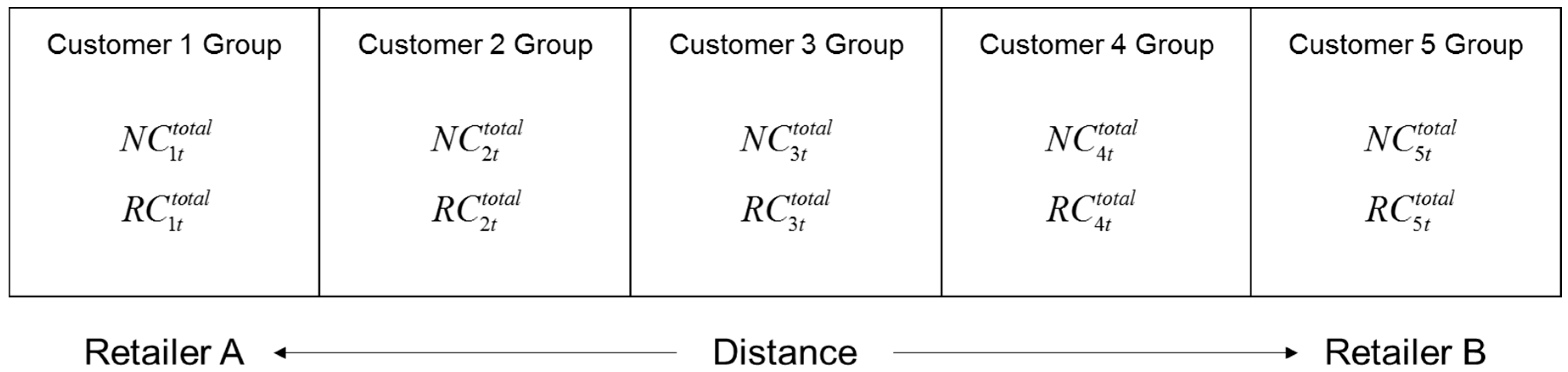
Figure 3.
Customer type of based on the residual value.

Figure 4.
Purchase probability for a new customer who knows about only one retailer.

Figure 5.
Simulation procedure.
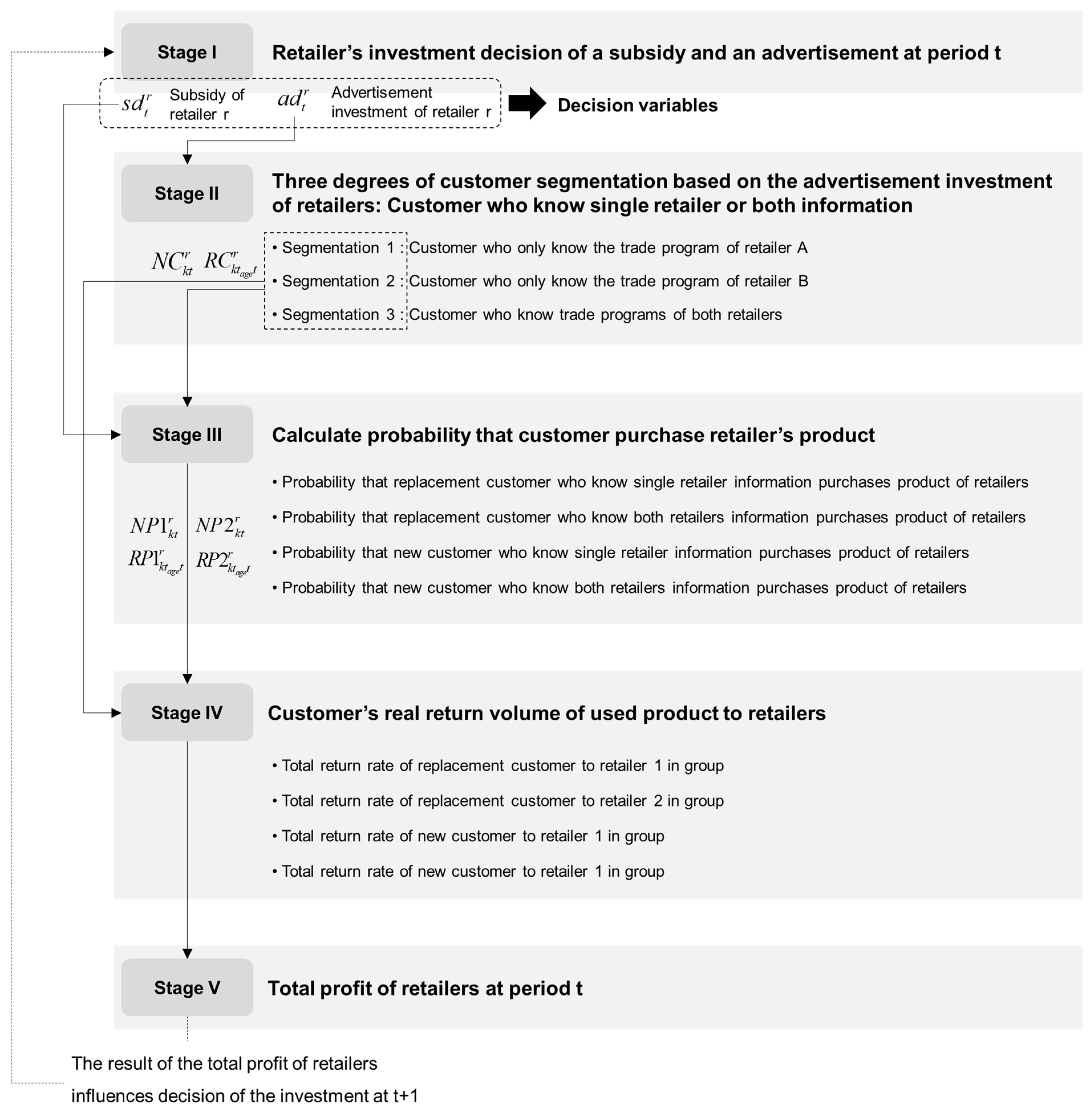
Figure 6.
Duopolistic competitive setting in this model.

Figure 7.
The results of the Fisher post hoc analysis for scenario 1 and 2.1 to 2.3.
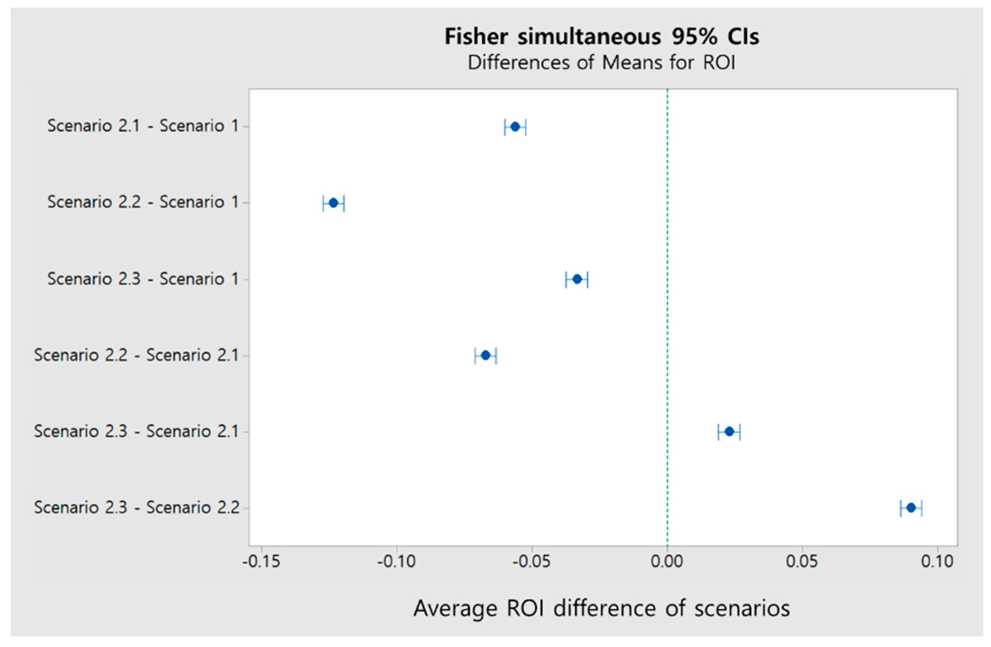
Figure 8.
The results of the Fisher post hoc analysis for scenario 3.1, 3.2 and 3.3.


Table 1.
Experiment parameters set.
| Parameters | Value |
|---|---|
| Uniform [0, ] | |
| 24 months | |
| Truncated Normal (min, max, mean, sd)~(100, 300, 200, 10) | |
| Uniform [0, ] | |
| $1400/unit | |
| $300/unit | |
| $1000 | |
| 0.3 | |
| $100 | |
| $500 | |
| $300 |
Table 2.
Design of experiment based on three scenarios.
| Scenarios | Investment Information of Competitor O: both Retailers Consider X: neither Retailer Considers △: one of the Retailers Considers | Retailer A | Retailer B |
|---|---|---|---|
| Scenario 1 | X | Investment strategy (1) | Investment strategy (1) |
| Scenario 2.1 | △ | Investment strategy (1) | Investment strategy (2) |
| Scenario 2.2 | △ | Investment strategy (1) | Investment strategy (3) |
| Scenario 2.3 | △ | Investment strategy (1) | Investment strategy (4) |
| Scenario 3.1 | O | Investment strategy (2) | Investment strategy (2) |
| Scenario 3.2 | O | Investment strategy (2) | Investment strategy (3) |
| Scenario 3.3 | O | Investment strategy (2) | Investment strategy (4) |
Table 3.
Experiment results of scenario 1 to scenario 2.3.
| Scenarios | Average Profit | Average Sales Volume | Average Investment in Advertisement | Average Investment in Subsidy | Return on Investment (ROI) | |||||
|---|---|---|---|---|---|---|---|---|---|---|
| Scenario 1 | 80,477 | 70,673 | 306 | 260 | 106,644 | 98,868 | 118,899 | 90,204 | 1.36 | 1.37 |
| Scenario 2.1 | 74,983 | 77,503 | 304 | 322 | 107,242 | 112,101 | 121,855 | 132,236 | 1.33 | 1.32 |
| Scenario 2.2 | 66,905 | 81,512 | 286 | 393 | 106,269 | 140,838 | 112,678 | 173,388 | 1.31 | 1.25 |
| Scenario 2.3 | 76,377 | 79,075 | 302 | 316 | 106,356 | 108,280 | 119,460 | 127,782 | 1.34 | 1.34 |
Table 4.
ANOVA results for scenarios 1 and 2.1 to 2.3.
| Basic Statistic Result of ROI of Retailer B | Analysis of Variance | ||||
|---|---|---|---|---|---|
| Scenarios | Average ROI | Standard Deviation | 95% C.I. | F-Value | p-Value |
| Scenario 1 | 1.37364 | 0.01629 | (1.37092, 1.37637) | 1410.99 | 0.00 |
| Scenario 2.1 | 1.31736 | 0.01728 | (1.31463, 1.32009) | ||
| Scenario 2.2 | 1.25012 | 0.02821 | (1.24739, 1.25285) | ||
| Scenario 2.3 | 1.34019 | 0.01389 | (1.33747, 1.34292) | ||
Table 5.
Experiment results of scenario 3.1 to scenario 3.3.
| Scenarios | Average Profit | Average Sales Volume | Average Investment in Advertisement | Average Investment in Subsidy | Return on Investment (ROI) | |||||
|---|---|---|---|---|---|---|---|---|---|---|
| Scenario 3.1 | 55,217 | 54,440 | 477 | 489 | 166,796 | 168,449 | 254,567 | 265,655 | 1.13 | 1.13 |
| Scenario 3.2 | 59,062 | 63,094 | 483 | 481 | 162,129 | 158,421 | 256,714 | 249,284 | 1.15 | 1.18 |
| Scenario 3.3 | 59,397 | 59,086 | 485 | 484 | 165,923 | 166,077 | 259,245 | 258,869 | 1.14 | 1.14 |
Table 6.
ANOVA results for scenarios 3.1, 3.2 and 3.3.
| Basic statistic result of ROI of retailer B | Analysis of variance | ||||
|---|---|---|---|---|---|
| Scenarios | Average ROI | Standard Deviation | 95% C.I. | F-Value | p-Value |
| Scenario 3.1 | 1.12685 | 0.02399 | (1.11713, 1.13657) | 1410.99 | 0.00 |
| Scenario 3.2 | 1.18999 | 0.1045 | (1.18027, 1.19971) | ||
| Scenario 3.3 | 1.14582 | 0.05718 | (1.13610, 1.15554) | ||
© 2017 by the authors. Licensee MDPI, Basel, Switzerland. This article is an open access article distributed under the terms and conditions of the Creative Commons Attribution (CC BY) license (http://creativecommons.org/licenses/by/4.0/).
Share and Cite
MDPI and ACS Style
Yoon, S.; Jeong, S. Investment Strategy in a Closed Loop Supply Chain: The Case of a Market with Competition between Two Retailers. Sustainability 2017, 9, 1712. https://doi.org/10.3390/su9101712
AMA Style
Yoon S, Jeong S. Investment Strategy in a Closed Loop Supply Chain: The Case of a Market with Competition between Two Retailers. Sustainability. 2017; 9(10):1712. https://doi.org/10.3390/su9101712
Chicago/Turabian StyleYoon, Sungwook, and Sukjae Jeong. 2017. "Investment Strategy in a Closed Loop Supply Chain: The Case of a Market with Competition between Two Retailers" Sustainability 9, no. 10: 1712. https://doi.org/10.3390/su9101712
Note that from the first issue of 2016, this journal uses article numbers instead of page numbers. See further details here.