Estimation and Healing of Coverage Hole in Hybrid Sensor Networks: A Simulation Approach


1
College of Information Science and Technology and Engineering Research Center of Digitized Textile and Fashion Technology, Ministry of Education, Donghua University, Shanghai 201620, China
2
Department of Automation, Shanghai Jiao Tong University, Shanghai 200240, China
*
Authors to whom correspondence should be addressed.
Sustainability 2017, 9(10), 1733; https://doi.org/10.3390/su9101733
Submission received: 27 July 2017
/
Revised: 19 September 2017
/
Accepted: 23 September 2017
/
Published: 26 September 2017
Abstract
:Nowadays, wireless sensor network which consists of numerous tiny sensors has been widely used. One of the major challenges in such networks is how to cover the sensing area effectively and maintain longer network lifetime with limited energy simultaneously. In this paper, we study hybrid sensor network which contains both static and mobile sensors. We divide monitoring area into Delaunay Triangulation (DT) by using of Delaunay theory, estimate static sensors coverage holes, calculate the number of assistant mobile sensors and then work out the positions of assisted mobile nodes in each triangle. Next, mobile sensors will move to heal the coverage holes. Compared with the similarity methods, the algorithm HCHA we proposed is simpler, the advantages of our algorithm mainly represents in the following aspects. Firstly, it is relatively simple to estimate coverage hole based on Delaunay in our proposed algorithm. Secondly, we figure out the quantitative number range of assisted sensors those need to heal the coverage holes. Thirdly, we come up with a kind of deployment rule of assisted sensors.
1. Introduction
With the development of the current technology and the extending of applied range of wireless sensor networks(WSNs), wireless sensor networks have gained widely attention for applying in natural disasters and some dangerous environment [1], such as earthquake stricken area and old-growth forest fire. Dangerous environment exits huge security risk for the rescuers if they need enter the primary scene, Fortunately, casting a mount of sensors to the monitoring area can not only solve the security risk problem but also make up WSNs networks to obtain the instant message of disaster area. However, the random deployment sensors may lead to the coverage holes and WSNs is the data-centered network. Thus, it is a worthy research to achieve efficient coverage.
Currently, numerous researchers have focused on the coverage problem and the classic papers including [2,3,4,5,6]. The main methods of increasing coverage include figuring out the coverage holes, healing the holes, and using adjustable radii to enlarge coverage. While the cost of enhancing the coverage is expensive, for instance, the former method requires all of the sensors have locomotion capabilities and the latter needs the sensors have several different power levers.
In this paper, we study the area coverage of hybrid sensor networks [7]. At first, we use static sensors to estimate the size of coverage hole and the number of assisted mobile sensor in the random distribution sensor network. Then deploying the assisted mobile nodes to heal the coverage holes. We assume that the initial network deployed a certain number of static nodes in the sensing field stochastically. The static nodes construct DT, then estimating the coverage holes in each triangle, and finding out the optimal positions of assisted nodes in every triangle. At last, the static sensors conduct the mobile sensors move to the optimal location to heal the coverage holes. Compared with the existing methods, our approach mainly shows several advantages as follows.
- Our calculation method of coverage is simpler than other works, the simulation of coverage ratio in Section 6 shows that our approach is better than previous works.
- We provide an auxiliary nodes deployment strategy that is applied to heal the coverage hole.
- We figure out the bound of assisted nodes number which is related to the ratio of .
The rest of the paper is organized as follows. In Section 2, we summarize the related work. In Section 3, we make some preparations and give out solution to the problem. Then, we propose the theoretical framework of the problem and show the analysis about the solution in Section 4. In Section 5, we elaborate our coverage algorithm. Performance evaluation and analysis are presented in Section 6. Conclusions and future work are given in the last part Section 7.
2. Related Work
In the WSNs, coverage is a fundamental but complicated problem all the time. For deterministic sensor deployment, coverage holes may not exist owns to the reasonable sensor layout, nevertheless the random distribution sensor always encounters many unexpected problems, for instance the redundant nodes and coverage holes. A lot of comprehensive studies about the redundancy and coverage have been done.
In paper [8], the authors discussed the effect of adjustable radius for the network lifetime. They proposed an algorithm based on learning-automata and equipped with a pruning rule, the algorithm is aimed to select a sensor which can adjust radius to satisfy a certain target coverage. The main idea of radius adaptive mechanism is to reduce the overlaps among sensing ranges while guarantee the QoS of coverage. However, radius adaptive mechanism is mainly used to solve the certain objective coverage problems, as how to apply it to more extensive coverage is a knotty question. Kang et al. at [9] estimated the number of coverage holes by detecting critical points on the boundary, calculated locations of new nodes by two kinds of models which are adjacent critical points and multi-adjacent critical points, as well as got the conclusion that patched sensor nodes should be deployed on the bisectors of boundary lines.
The hybrid network which contained both static and mobile sensors was studied in paper [10,11,12,13,14,15,16]. Wang et al. [10] employed the geometrical approaches, and the mainly steps including divided monitoring area into many cells by Voronoi diagram [11], estimated the coverage holes by static sensors and commanded mobile sensors to move to the target location to heal the holes. But they did not propose the detail scheme about how to work out the coverage holes. In the process of biding the mobile sensors, two mobile guidelines those were Distance-based and Price-based were came up by them. The Distance-based scheme mainly took the moving distance into consideration, the assistant sensor moves or not depends on the distance between server and target location. The Price-based approach was based on the cost, due to move different mobile sensors have different cost, the cheapest mobile sensor would have priority to heal the coverage hole. Besides, they also provided a Multiple Healing Detection algorithm to deal with the multiple healing problem. In paper [12], the authors developed two sets of distributed protocols [13] for controlling the movement path of sensors and provided three kind of target locations calculated algorithms.
Wu et al. [5] proposed the DT-Score algorithm which was a two phases method to maximize the coverage of an area with obstacles. At the first phase, they used contour-based deployment to estimate the coverage holes, what important is that the deployment has an excellent performance of coverage holes detecting about the obstacles and area boundary. It is important to deploy an excellent performance of coverage holes detecting about the obstacles and area boundary. In the second phase, the deployment method applied the DT to the uncovered area, after calculating the candidate positions of assistant sensors, they scored the candidate position and chosen the high scores positions to locate assistant sensor.
Ghosh et al. [14] provided the COVEN algorithm to enhance coverage, they exploited the Voronoi diagram to achieve accurate calculation about the coverage holes. The method divided the detecting field into many cells and then divided every cell into several triangles, next discussed the relationship between sensor radius and Voronoi edge , then worked out the uncovered area in every cell, finally dispatched the assisted sensors to heal the coverage holes. The positions of assisted nodes in COVEN algorithm must satisfy three conditions as follows:
- lies on the line that bisects the inner angle formed by which is Voronoi vertex;
- is located in the Voronoi polygon;
- .
The frame of our paper is similar with the paper [14]. The general idea is to detect the coverage holes in every triangle, then dispatch nodes to heal the holes. What different from previous work is as follows. Firstly, compared with the existed approaches mentioned above, we provide one simpler method to estimate the coverage hole. Secondly, we work out the bound of assisted nodes number and provide the minute deployment rules for the assisted sensors.
3. Preliminaries
The WSNs is consisted of many mobile sensors and static sensors, the fundamental problem of this paper is how to enhance the coverage by finding and healing coverage holes. Next, we will introduce some preparative knowledge which is used in the following analysis.
3.1. Communication and Sensing Models
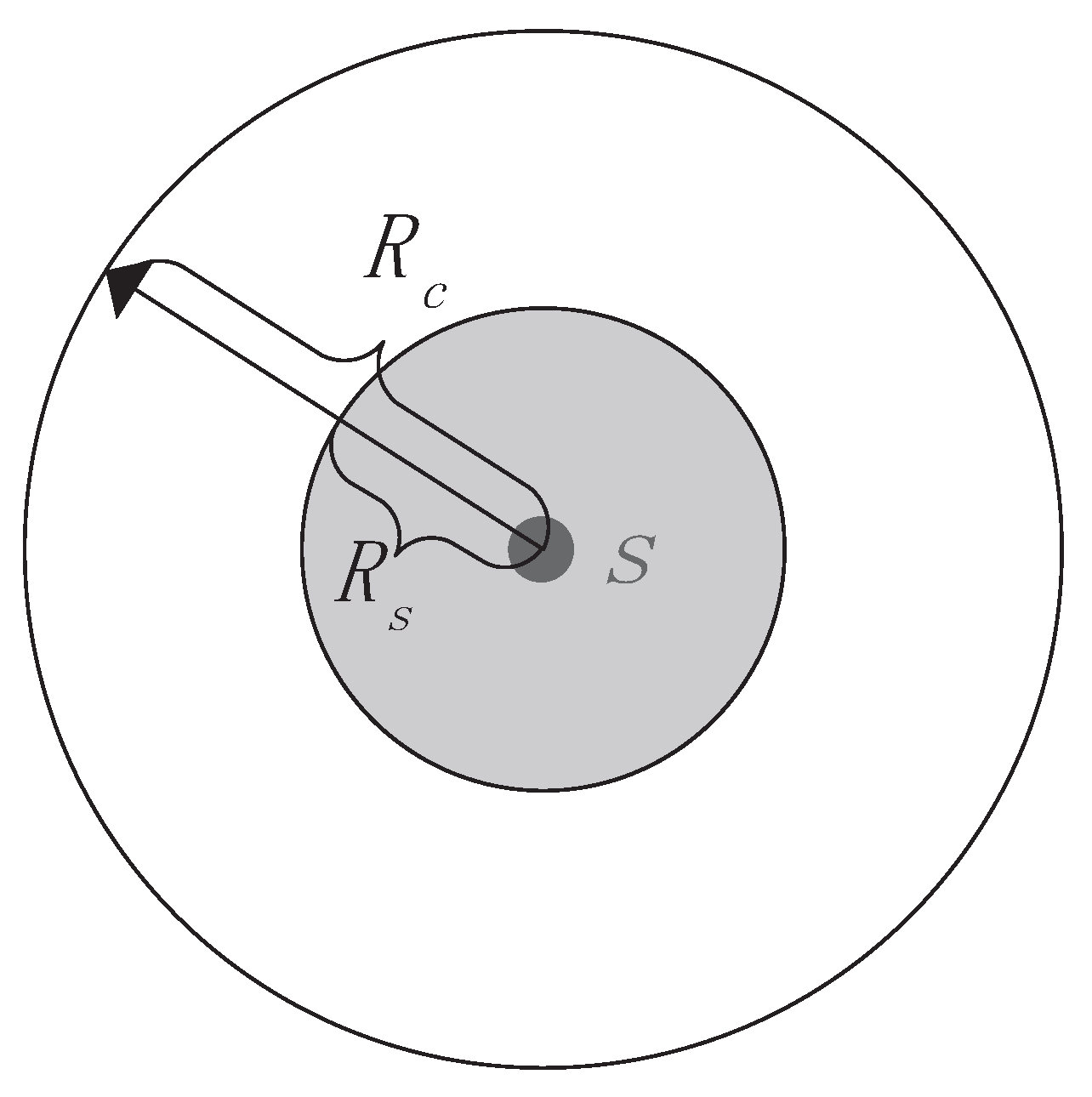
Each sensor has communication capacity and sensing capacity, is defined as communication radius and is defined as sensing radius, Figure 1. shows the communication and sensing models. If and only if the distance between two sensors is within , they can communicate with each other, otherwise the node is isolated. Tian et al. [17], Wang et al. [18], Zhang et al. [19] proved that if a convex region is completely covered by a set of nodes, the communication graph consisting of these nodes is connected when .
3.2. DT and Related Definitions
DT is an important data structure in computational geometry [20]. The most significant property we use in this paper is that (1) maximum empty circle characteristic which means any four points do not construct a circle; (2) maximize the minimum angle which means the composition of triangle is reasonable and not too narrow. We can detect the coverage hole in the each delaunay triangle by discussing the and the circumcenter of triangle. If is not covered by the sensor node of triangle, there will exist coverage holes in the triangle. Given N static sensors , , ⋯, we can get the DT. For example, we choose 50 random nodes to generate DT by MATLAB as shown in Figure 2.
3.3. Problem Statement
The coverage of the wireless sensor network can be divided into area coverage, point coverage and barrier coverage. Point coverage requires specific points covered, are coverage needs entire region covered and barrier coverage aims to detect the intruders who try to cross the network [21]. In this paper we mainly discuss the areas coverage under circumstance of nodes randomly deployed. At first, assuming a 100 m × 100 m scene and deploying a certain number of static sensors randomly in this area. Obviously, because of some places are covered densely while others sparsely, the current coverage is not the optimal. In this article, we studied the problem of how to detect and heal the coverage holes, and we need to solve the following three subproblems:
- Estimate the coverage holes in the sensing areas more simply and accurately.
- Figure out the bound of assisted sensors which are used to heal the coverage holes in every triangle.
- Work out the optimal positions of assisted sensors.
To simplify the analysis of the problem later, we assume that all sensors’ sensing range is a circle with the radius of , is defined as communication range. In order to facilitate reading, we introduce some parameters in Table 1:
4. Theoretical Analysis
4.1. Repair DT
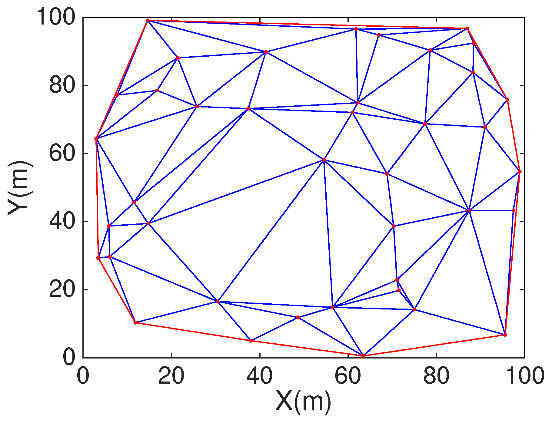
The randomly distributed nodes in the 100 m × 100 m scene can construct DT. According to the properties of Delaunay, we know that DT is convex as shown in Figure 2. The coverage holes in the boundary cannot be detected due to the triangle cannot be formed in marginal area. In order to solve this question, we need to deploy some nodes in boundary and corner of the area, which can construct the DT to fill the monitoring area as shown in Figure 3.
4.2. Estimation of Coverage Holes
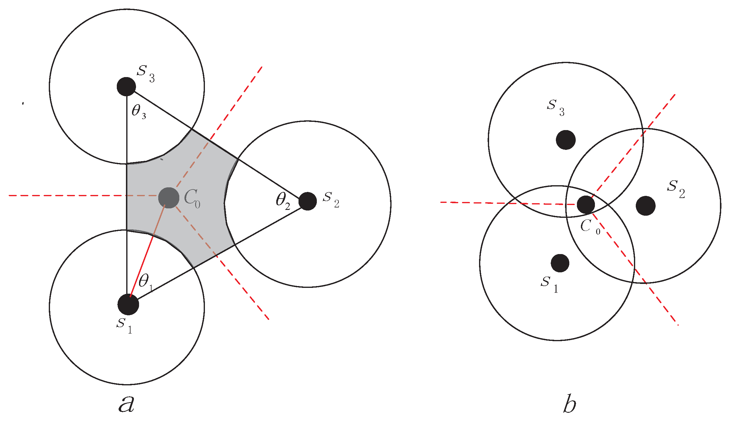
Deploying the sensors randomly will lead to coverage holes, we introduce Delaunay to estimate the coverage holes. is the circumcenter of the and the distance is circumradius R as shown in Figure 4.
Theorem 1.
If then there does not exist coverage hole between the three sensors, if the is an acute triangle and then there must exist coverage holes between three sensors [22].
Proof of Theorem 1.
We know is the circumcenter of , according to geometry we can get conclusion easily that the distance between and is equal, so if the is covered by sensor , then must be covered by neighbour nodes and as as demonstrated in Figure 5b. It is apparently that the triangle area constructed by and its two neighbours do not exist coverage holes. ☐
If the is not covered by node S just as shown in Figure 5a, then there must exist coverage holes, we should estimated the uncovered shadow area and worked out how many additional mobile sensors should healed the coverage hole. Assuming that each sensor’s location is known, then , and the sector area can be calculated as follow:
the area of :
According to the (1) and (2), can be derived as follow:
From (1)–(3) we can estimate the number of additional mobile sensors which is needed to heal the coverage holes, define then
Input parameter () to round the number of assisted sensor.
4.3. The Bound of Assisted Nodes Number
Nodes communicate with each other is the prerequisite of constructing DT, based on the triangular set we know that the number of assisted nodes is related to the relationship between and . In the following theorem, we present the theoretical bound of assisted nodes numbers. In order to normalize the problem, we suppose that (), if and only if nodes can communicate with each other i.e., , now which is one of special scenario from general condition (5), and can provide the upper bound of assisted nodes numbers. Thus, we have the bound of assisted nodes number:
Theorem 2.
If and only if nodes can communicate with each other, the bound of assisted sensors number () in the triangle can be derived as follow:
where ρ= and .
Proof of Theorem 2.
When , and are far from each other with the distance , which means is a regular triangle with side length . Easily we can get , from (5) we can get , then we can get . When the is zero then the lower bound of assisted sensors is zero, so the bound of assisted sensors can be derived: ☐
4.4. Position Of Assisted Sensors
Theorem 3.
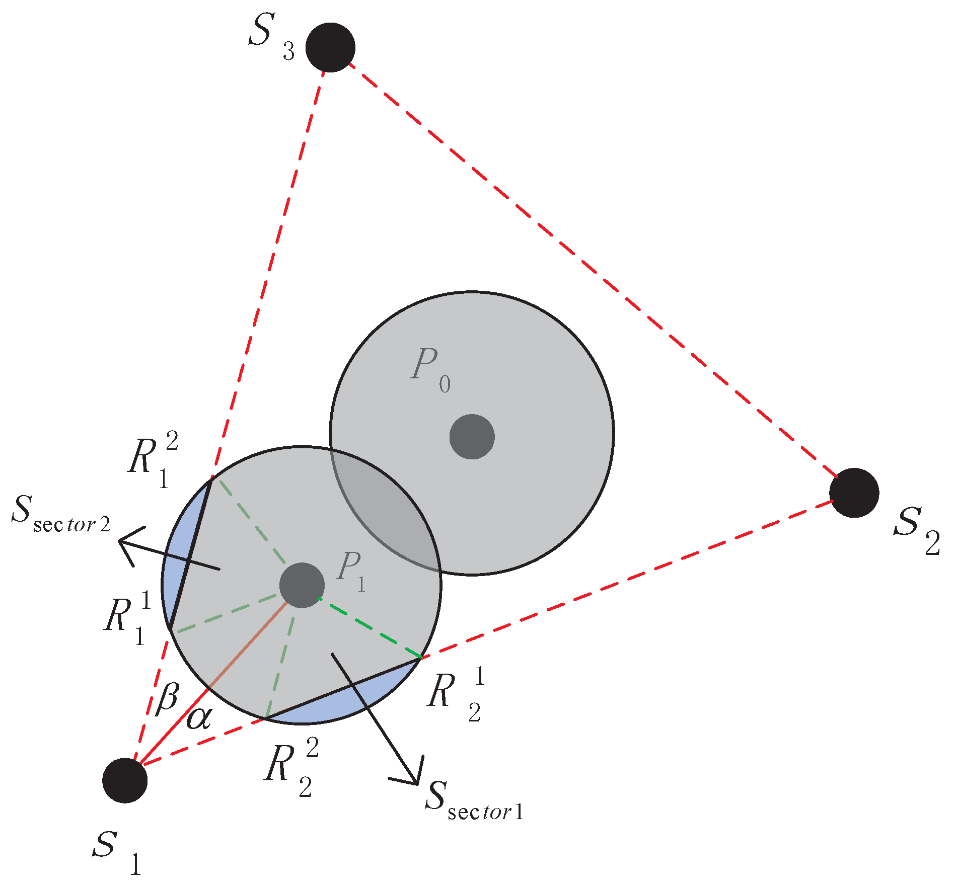
If only need one assisted node , select inner centre of as the position of first assisted sensor, When then the position of assisted sensor must lie on the angle bisector of , which is the line connects to .
Proof of Theorem 3.
First, when there is only one sensor enough to cover the , apparently it should take the inner center of as the first assisted sensor location and where is the optimal choice, for the reason that has the same distance from three sides which can achieve maximal coverage in the triangle. Second, in order to proof that lies at angular bisector , we introduce two assisted angles , if we can proof that only when , the bow area is minimal then we can deduce that is on the angle bisector . Assume that the distance between and is d, we can get the area of and , and .
we can get the , in a similar way can be got. Finally, the blue area
According to the extremum theorem of the two function, easily we can get when , is least, thus , so is the angular bisector of . ☐
We proved that assisted sensor must lie on the angle bisector of which is constituted by three neighbor nodes, next we determine the concrete location of sensor node.
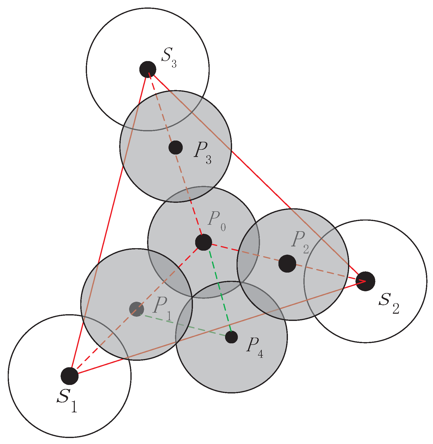
If there only need one assisted node to heal the coverage hole, as we have claimed before that take inner center as the position of first assisted sensor as shown in Figure 5. If , first compare the distance , and . Assumed that , then the second assisted sensor should lie on line , if then for the overlap with node and is minimum. If , then . If the third assisted sensor is needed, its position is on line and the fourth node is on line at , the fifth node lies on perpendicular bisector of and . Additionally, the distance far from is just as Figure 6 demonstrates, the rest can be deduced by the same manner. In this way, the coverage is relative maximization and redundant coverage is relative minimization in current triangle.
5. Heal Coverage Holes Algorithm
In this section, we will integrate the several subproblems we have solved above and propose the Heal Coverage Holes Algorithm( HCHA) detailed. The network we research is hybrid, which consists of both static and mobile sensors. During the network initialization, static sensors construct the DT.
Pseudo-code is given in Algorithms 1 and the process is illustrated in Figure 7.
| Algorithm 1 deploy assisted node in each triangle |
|
Step 1. Select the node with maximum energy as the head node in each triangle. In order to balance the energy consumption, we set the sensor which is selected as head node will not attend again in head selection of other neighbour triangles. The head node gathers the relevant information including current energy, position from the remaining two static sensors of the triangle and estimates coverage holes, the number of the assisted sensors as well as the position of assisted sensors. Then head node broadcasts the information of calculation results with a distance threshold which is used to limit the hop ( Package Information ).
Step 2. Once mobile sensor receives the data package, it will compare the distance with the , if , send message which contains location, energy information and ID back to the head node by multiple hops, and continue to broadcast Package Information. If , transfers the message back to the head node only and stops broadcasting Package Information.
Step 3. Head node receives the information of mobile nodes around, chooses the optimal node based on the energy and position information, then sends command.
Step 4. Lastly, Mobile node judges whether itself needs to move by the command.
6. Performance Evaluation and Analysis
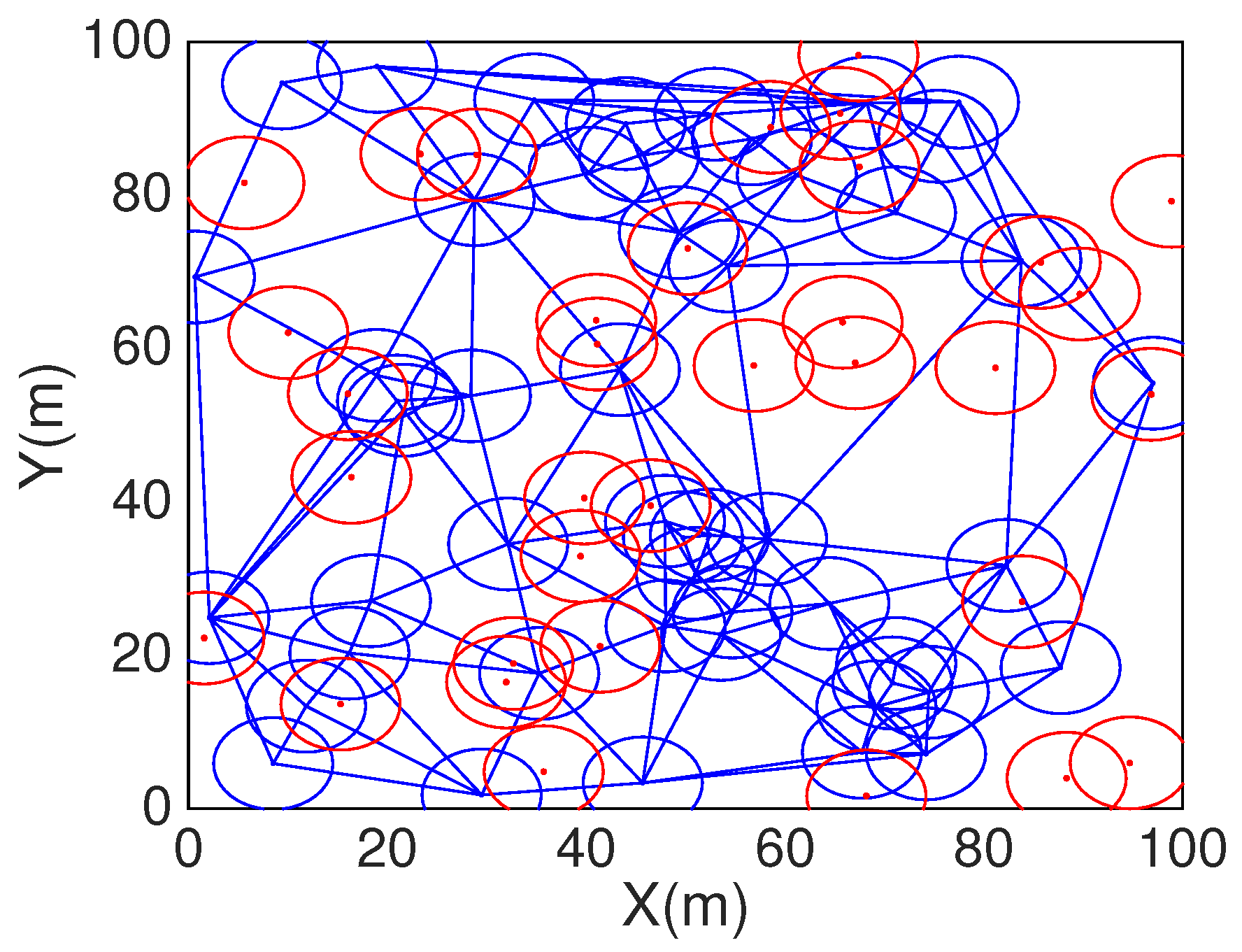
In this section, we will conduct comparative simulations about our algorithm HCHA, the main simulation platform we used is Matlab. In order to make a remarkable contrast, we compare HCHA deployment with the random deployment, COVEN deployment in paper [17] and DT-Score deployment in paper [19]. The simulation area we choose is 100 m × 100 m and sensing radius is 5 m, is 0.5, red nodes represent mobile sensors and blue represent static sensors. Because COVEN, DT-Score and HCHA have different abilities to be estimated, so we can only set some same parameters such as number of static sensors 50, as to the number of mobile sensors, it need to be calculate by COVEN and HCHA separately, which is not decide by manual setting, as well as DT-Score calculate the candidate positions. Coverage simulation results are demonstrated in Figure 8, Figure 9, Figure 10, Figure 11, Figure 12, Figure 13, Figure 14, Figure 15 and Figure 16.
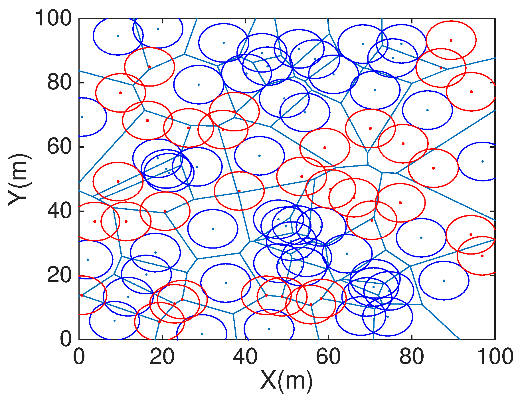
Figure 8 and Figure 10 are randomly deployment and HCHA deployment with 50 static sensors and 72 mobile sensors, which number is figured out by HCHA. Figure 9 is the COVEN deployment with 50 mobile sensors and 58 mobile sensors, which are figured out by COVEN. Figure 11 is the HCHA deployment after DT repaired with 50 static sensors and 88 mobile sensors, which number is calculated by HCHA after the DT paired, and the DT repaired aims to cover the area boundary. In Figure 10 we can find the area boundary is not covered by the sensors both of static and mobile, but in Figure 11 which is after the DT repair, all the area boundary is covered by sensors.
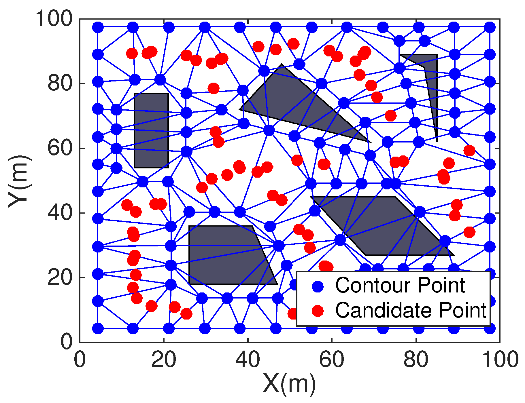
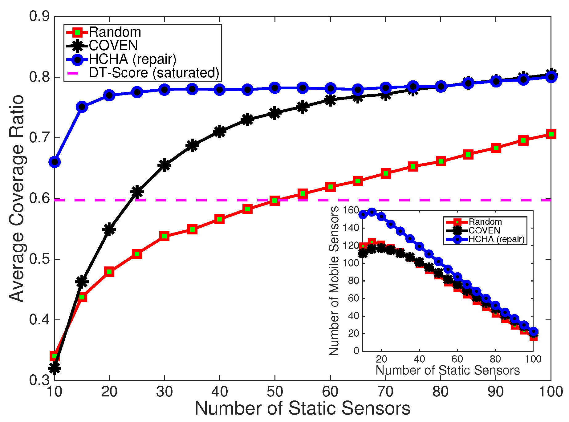
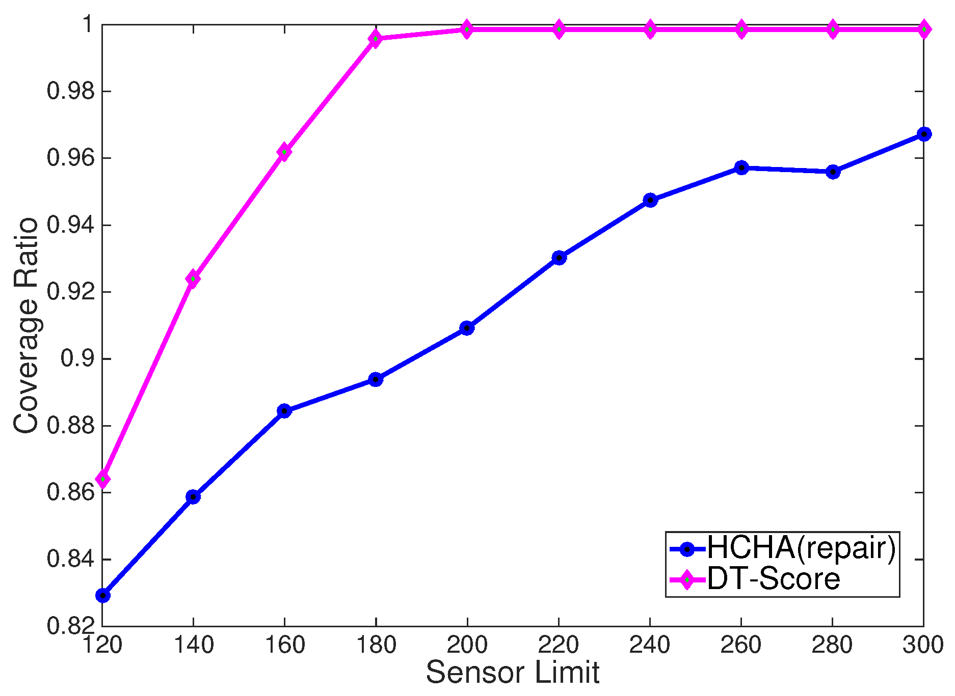
In order to compare HCHA with DT-Score, we construct obstacles scenario as shown in Figure 12. For the same one obstacles exist scenario, Figure 13 shows the coverage with DT-Score, the blue point represent contour point and red represent candidate point, Figure 14 is the coverage with HCHA after DT repair. Figure 15 shows four algorithms including COVEN, DT-Score, random and our HCHA coverage ratio in the without obstacles exist scenario, for the main picture x-label is the number of static sensors and y-label is corresponding coverage ratio, the subgraph in the bottom right corner shows the relationship between the number of static sensors and mobile sensors.
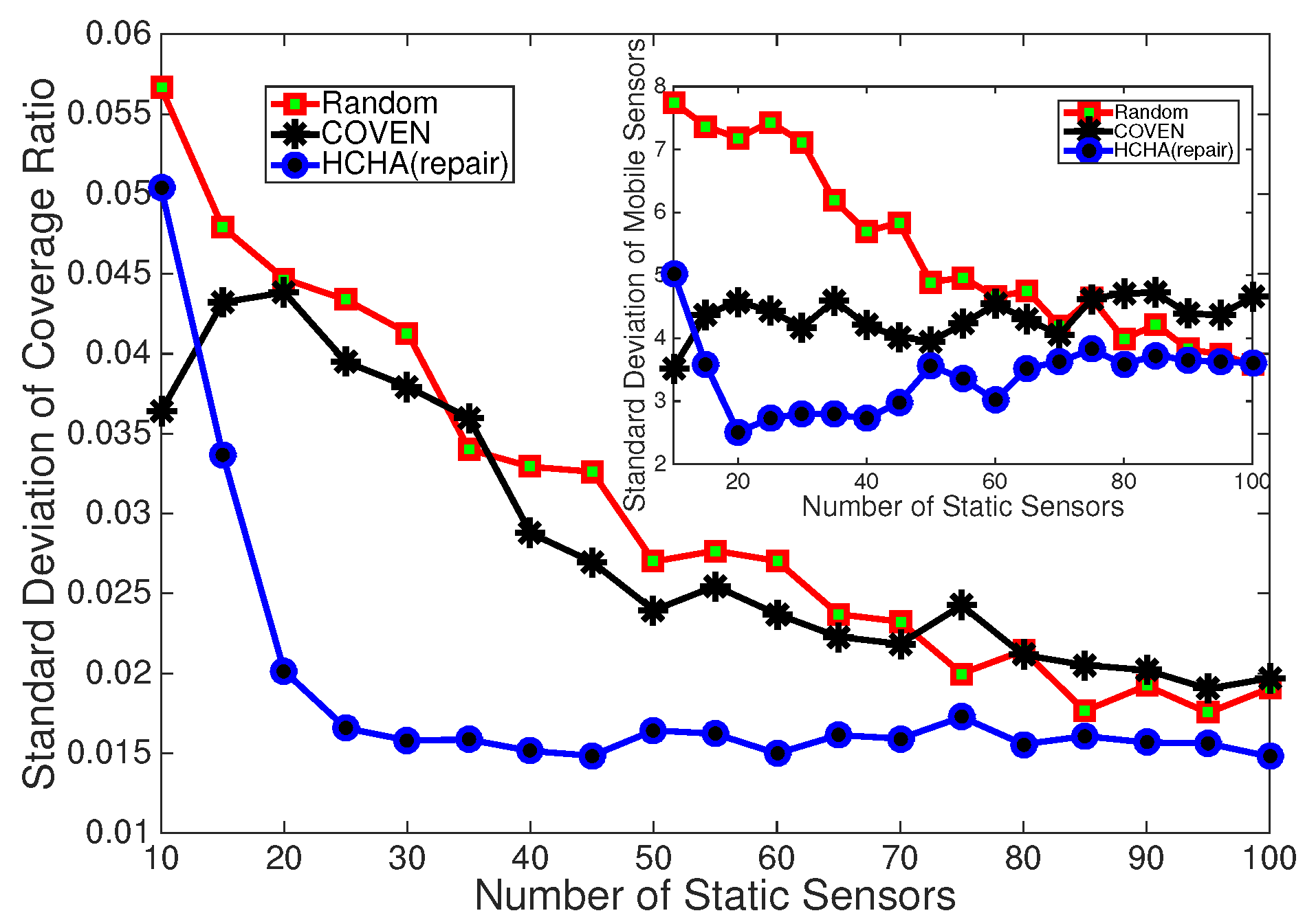
In Figure 15 we repeat the simulation for 200 times and take the average to plot the line chart, because the static nodes is deployed randomly, which leads to the simulation result is different every time. It can be seen that HCHA provides almost more coverage than COVEN when there are 10 static nodes, while it requires about 50% more mobile nodes than COVEN. And the gap shrinks with the increasing of static nodes. It is also important that HCHA can detect and heal coverage holes well even when there is a little number of static nodes, and COVEN cannot provide better coverage by increasing the mobile nodes in such circumstances. This means HCHA is less dependent on the density of static nodes than COVEN. In Figure 16 we statistic the standard deviation of 200 times simulation, and from the results we discover HCHA is more stable than Random and COVEN. As to the obstacles exist condition, the coverage of HCHA and DT-Score is shown in Figure 17. It is easy to learn that the DT-Score has a better performance in the obstacles exist scenarios. Because our HCHA is proposed without the consideration of obstacles condition, and this condition will be researched in our future work.
Our HCHA follow three key steps. Step one, static sensors construct DT. Step two, select head node to calculate coverage holes and find optimal position in the triangle. Step three, head nodes order mobile sensors to heal coverage holes. Compared to the COVEN, our algorithm exists some advantages. Firstly, our coverage holes detected algorithm based on Delaunay is relatively simpler than COVEN in three aspcts:
- The coverage holes detecting. The COVEN algorithm divide the area based on the Voronoi diagram, as the result, the area is divided into many cells, and then divided every cell into several triangles to detect and calculate coverage holes. However, our HCHA algorithm based on the DT, which can divide the area in to triangles immediate, the steps are less than COVEN.
- The assistant number calculation. The COVEN algorithm calculation the assistant sensors number need consider the sum of triangles those belong to the same one cell, but our HCHA can calculate every triangle directly.
- The assistant sensor position finding. The COVEN finding the assistant sensor position based on the cross-regional but our HCHA algorithm is based on each triangle unit.
Secondly, the COVEN which mainly calculated coverage holes in every Voronoi polygon and every mobile sensor is located in the angle bisector corresponding to each Voronoi veretx. However, HCHA estimates full coverage holes in a triangle, assisted sensor deployed in each triangle and considers multiple nodes deployment. The assisted nodes deployment strategy of HCHA and COVNE is shown in Figure 13 and Figure 14. Besides we work out the concrete amount of assisted nodes in every triangle corresponding to different ratio .
Thirdly, compared to DT-Score, our HCHA has a better evaluation in the without obstacles condition, but for the obstacles scenario, we need pay more attention to enhance the coverage.
7. Conclusions and Future Work
In this paper, we study the coverage problem in hybrid WSNs and we give HCHA algorithm based on Delaunay to estimate as well as heal coverage holes in the monitoring area, besides we solve the boundary coverage holes estimation and consider multiple assisted nodes healing deployment strategy. In order to generalize problems, we also give the quantitative range of assisted nodes which is related to parameter k, where k is the ration between and .
For the future work, we are prepared to research directional sensor networks (DSN) and how to enhance the coverage ratio with the random distribute sensors in the obstacles exist scenario. The coverage of DSN is related to node coordinate, , working direction and angle of view, which is different from Omnidirectional sensor network.
Acknowledgments
This work is supported by the NSF of China under Grant No. 61772130, No. 61301118 and No. 71171045; the International S & T Cooperation Program of Shanghai Science and Technology Commission under Grant No. 15220710600; the Innovation Program of Shanghai Municipal Education Commission under Grant No. 14YZ130; and the Fundamental Research Funds for the Central Universities. This paper is an extended version of our conference paper: Coverage Holes Detecting and Healing in Hybrid Wireless Networks [23].
Author Contributions
The work presented in this paper is a collaborative development by all of the authors. Guanglin Zhang and Chengsi Qi contributed to the idea of the incentive mechanisms and designed the algorithms. Wenqian Zhang, Jiajie Ren, and Lin Wang developed and analyzed the experimental results. All authors contributed to the organization of the paper including writing and proofreading.
Conflicts of Interest
The authors declare no conflict of interest.
References
- Tuna, F.; Gungor, V.C.; Gulez, K. An autonomous wireless sensor network deployment system using mobile robots for human existence detection in case of disasters. Ad Hoc Netw. 2014, 13, 54–68. [Google Scholar] [CrossRef]
- Liang, J.; Liu, M.; Kui, X. A survey of coverage problems in wireless sensor networks. Sens. Transducers 2014, 10, 163–174. [Google Scholar]
- Mahboubi, H.; Moezzi, K.; Aghdam, A.G.; Sayrafian-Pour, K.; Marbukh, V. Distributed deployment algorithms for improved coverage in a network of wireless mobile sensors. IEEE Trans. Ind. Inform. 2014, 13, 54–68. [Google Scholar] [CrossRef]
- Khoufi, I.; Minet, P.; Laouiti, A.; Mahfoudh, S. Survey of deployment algorithms in wireless sensor networks: Coverage and connectivity issues and challenges. Int. J. Autono. Adapt. Commun. Syst. (IJAACS) 2014. Available online: https://hal.inria.fr/hal-01095749 (accessed on 25 September 2017).
- Wu, C.H.; Lee, K.C.; Chung, Y.C. A Delaunay triangulation based method for wireless sensor network deployment. Comput. Commun. 2007, 30, 2744–2752. [Google Scholar] [CrossRef]
- Zhang, G.; You, S.; Ren, J.; Wang, L. Local Coverage Optimization Strategy Based on Voronoi for Directional Sensor Networks. Sensors 2016, 16, 2183. [Google Scholar] [CrossRef] [PubMed]
- Wang, Y.-C. A two-phase dispatch heuristic to schedule the movement of multi-attribute mobile sensors in a hybrid wireless sensor network. IEEE Trans. Mob. Comput. 2014, 13, 709–722. [Google Scholar] [CrossRef]
- Mohamadi, H.; Salleh, S.; Razali, M.N.; Marouf, S. A new learning automata-based approach for maximizing network lifetime in wireless sensor networks with adjustable sensing ranges. Neurocomputing 2015, 153, 11–19. [Google Scholar] [CrossRef]
- Kang, Z.; Yu, H.; Xiong, Q. Detection and recovery of coverage holes in wireless sensor networks. J. Netw. 2013, 8, 822–828. [Google Scholar] [CrossRef]
- Wang, G.; Cao, G.; Berman, P.; La Porta, T.F. Bidding protocols for deploying mobile sensors. IEEE Trans. Mob. Comput. 2007, 6, 563–576. [Google Scholar] [CrossRef]
- Liu, J.; Sun, X.; Xing, H.; Zhao, Y. Coverage area detection based on voronoi diagram in wireless sensor network of metro. In Proceedings of the International Conference on Machine Learning and Cybernetics, Jeju, Korea, 10–13 July 2016; pp. 410–415. [Google Scholar]
- Wang, G.; Cao, G.; La Porta, T.F. Movement-assisted sensor deployment. IEEE Trans. Mob. Comput. 2007, 5, 640–652. [Google Scholar] [CrossRef]
- Pantazis, N.A.; Nikolidakis, S.A.; Vergados, D.D. Energy-efficient routing protocols in wireless sensor networks: A survey. IEEE Commun. Surv. Tutor. 2013, 15, 551–591. [Google Scholar] [CrossRef]
- Ghosh, A. Estimating coverage holes and enhancing coverage in mixed sensor networks. In Proceedings of the 29th Annual IEEE International Conference on Local Computer Networks, Tampa, FL, USA, 16–18 November 2004; pp. 68–76. [Google Scholar]
- Zhang, G.; Liu, J.; Ren, J.; Wang, L.; Zhang, J. Capacity of Content-Centric Hybrid Wireless Networks. IEEE Access 2017, 5, 1449–1459. [Google Scholar] [CrossRef]
- Zhang, G.; Liu, J.; Ren, J. Multicast capacity of cache enabled content-centric wireless Ad Hoc networks. China Communications 2017, 14, 1–9. [Google Scholar] [CrossRef]
- Tian, D.; Georganas, N.D. Connectivity maintenance and coverage preservation in wireless sensor networks. Ad Hoc Netw. 2005, 3, 744–761. [Google Scholar] [CrossRef]
- Wang, X.; Xing, G.; Zhang, Y.; Lu, C.; Pless, R.; Gill, C. Integrated coverage and connectivity configuration in wireless sensor networks. In Proceedings of the 1st International Conference on Embedded Networked Sensor Systems, Los Angeles, CA, USA, 5–7 November 2003; ACM: New York, NY, USA, 2003; pp. 28–39. [Google Scholar]
- Zhang, H.; Hou, J.C. Maintaining sensing coverage and connectivity in large sensor networks. Ad Hoc Sens. Wirel. Netw. 2005, 1, 89–124. [Google Scholar]
- Fortune, S. Voronoi diagrams and delaunay triangulations. Comput. Euclidean Geom. 1992, 1, 1–12. [Google Scholar]
- Saipulla, A.; Westphal, C.; Liu, B.; Wang, J. Barrier coverage of line-based deployed wireless sensor networks. In Proceedings of the INFOCOM 2009, Rio de Janeiro, Brazil, 19–25 April 2009; pp. 127–135. [Google Scholar]
- Ma, H.C.; Sahoo, P.K.; Chen, Y.W. Computational geometry based distributed coverage hole detection protocol for the wireless sensor networks. J. Netw. Comput. Appl. 2011, 34, 1743–1756. [Google Scholar] [CrossRef]
- Qi, C.; Zhang, G.; Li, D.; Ren, J. Coverage Holes Detecting and Healing in Hybrid Wireless Networks. In Proceedings of the 10th EAI International Conference on Mobile Multimedia Communications, Chongqing, China, 13–14 July 2017. [Google Scholar]
Figure 1.
Communication and sensing models.

Figure 2.
Delaunay Triangulation (DT).

Figure 3.
DT Repaired.
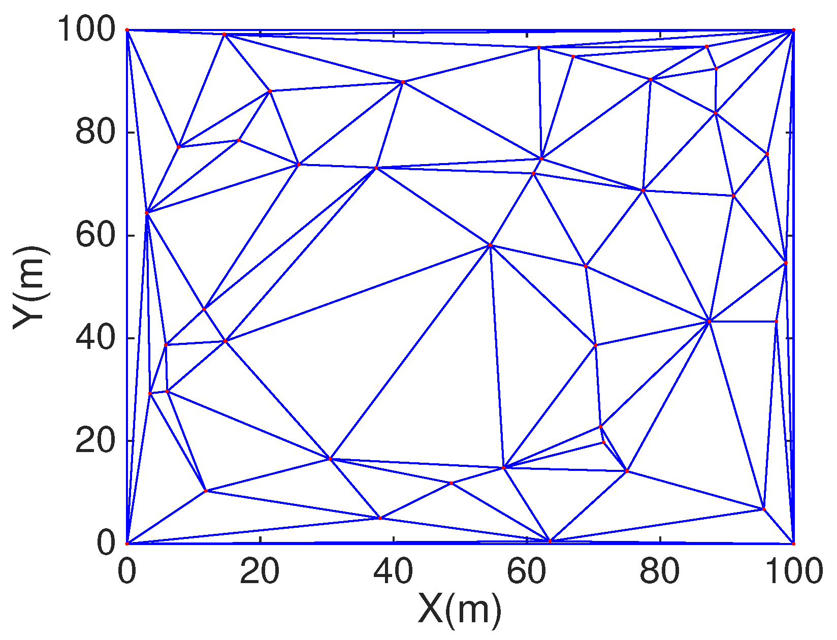
Figure 4.
Nodes construct triangle.
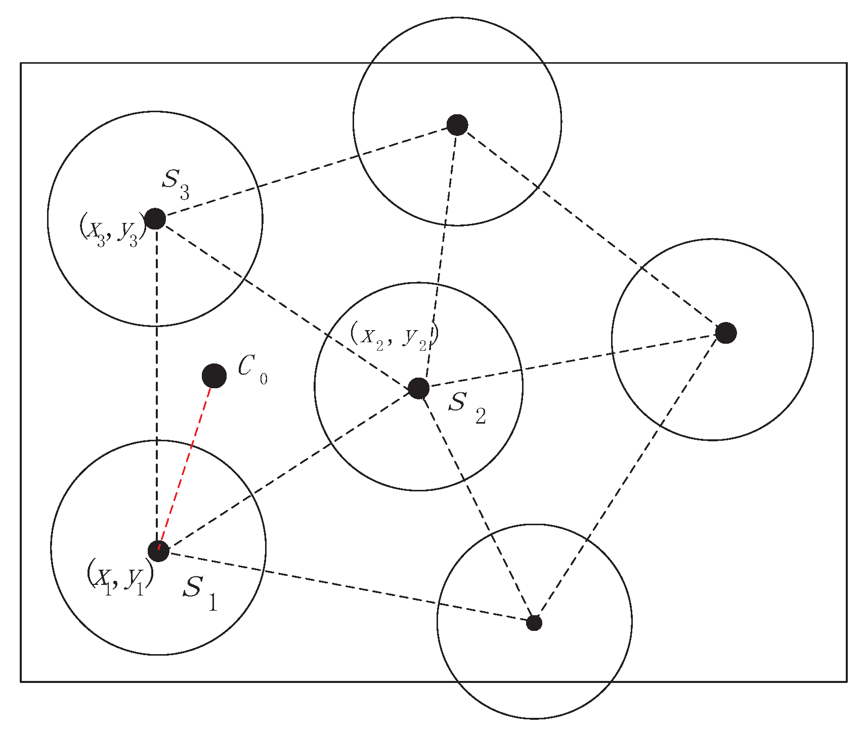
Figure 5.
Coverage holes estimated.

Figure 6.
Node lies in the angle bisector.

Figure 7.
Position of assisted sensor.

Figure 8.
Random deployment of 50 static sensors coupled with 72 mobile sensors.

Figure 9.
COVEN deployment of 50 static sensors coupled with 58 mobile sensors.

Figure 10.
HCHA deployment of 50 static sensors coupled with 72 mobile sensors.
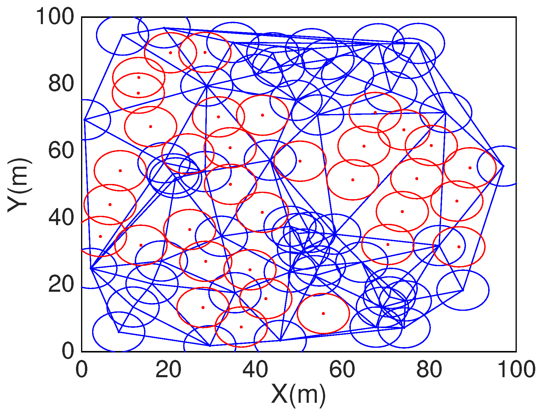
Figure 11.
HCHA(Repair DT) deployment of 50 static sensors coupled with 88 mobile sensors.
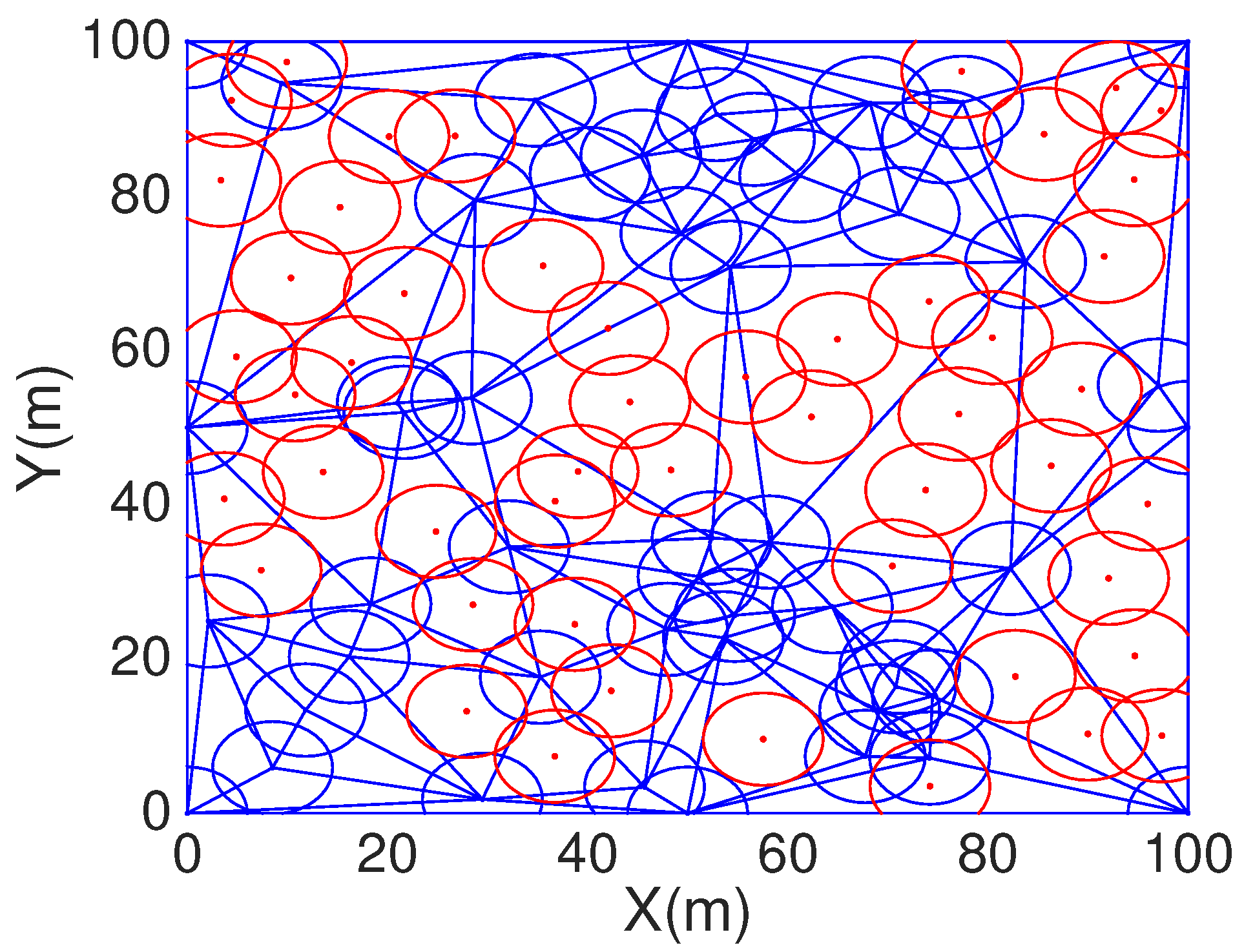
Figure 12.
Obstacles.
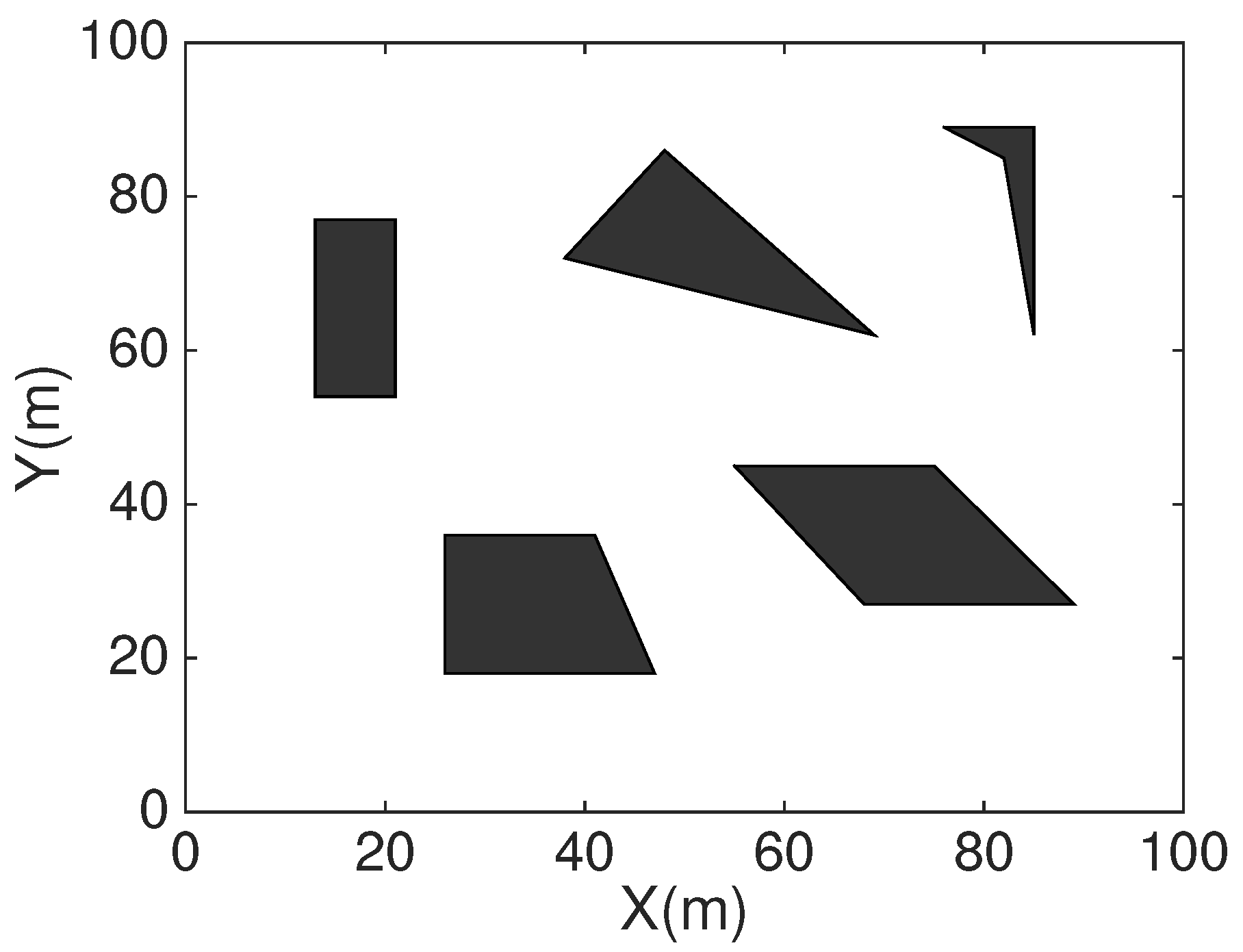
Figure 13.
Obstacle coverage with DT-Score.

Figure 14.
Obstacle coverage with HCHA.
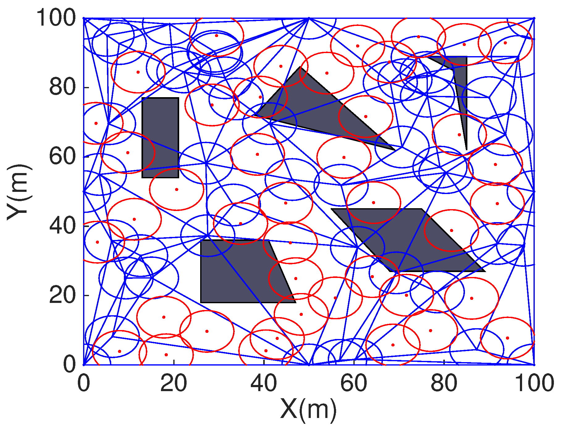
Figure 15.
Coverage ratio without obstacles (200 times).

Figure 16.
The standard deviation of simulation (200 times).

Figure 17.
Coverage ratio with obstacles (200 times).


Table 1.
Main Notations.
| Notation | Definition |
|---|---|
| , | Static sensor and mobile sensor |
| Angle of three Delaunay triangle | |
| Sensing radius and communication radius | |
| Position of mobile assisted sensor | |
| The circumcenter of the | |
| Uncovered area of the triangle | |
| Euclidean distance between and | |
| Input parameter to round the number of assisted sensors |
© 2017 by the authors. Licensee MDPI, Basel, Switzerland. This article is an open access article distributed under the terms and conditions of the Creative Commons Attribution (CC BY) license (http://creativecommons.org/licenses/by/4.0/).
Share and Cite
MDPI and ACS Style
Zhang, G.; Qi, C.; Zhang, W.; Ren, J.; Wang, L. Estimation and Healing of Coverage Hole in Hybrid Sensor Networks: A Simulation Approach. Sustainability 2017, 9, 1733. https://doi.org/10.3390/su9101733
AMA Style
Zhang G, Qi C, Zhang W, Ren J, Wang L. Estimation and Healing of Coverage Hole in Hybrid Sensor Networks: A Simulation Approach. Sustainability. 2017; 9(10):1733. https://doi.org/10.3390/su9101733
Chicago/Turabian StyleZhang, Guanglin, Chengsi Qi, Wenqian Zhang, Jiajie Ren, and Lin Wang. 2017. "Estimation and Healing of Coverage Hole in Hybrid Sensor Networks: A Simulation Approach" Sustainability 9, no. 10: 1733. https://doi.org/10.3390/su9101733
Note that from the first issue of 2016, this journal uses article numbers instead of page numbers. See further details here.