Energy Substitution Effect on China’s Heavy Industry: Perspectives of a Translog Production Function and Ridge Regression

1
School of Management, China Institute for Studies in Energy Policy, Collaborative Innovation Center for Energy Economics and Energy Policy, Xiamen University, Xiamen 361005, China
2
The School of Economics, China Center for Energy Economics Research, Xiamen University, Xiamen 361005, China
*
Author to whom correspondence should be addressed.
Sustainability 2017, 9(11), 1892; https://doi.org/10.3390/su9111892
Submission received: 17 September 2017
/
Revised: 14 October 2017
/
Accepted: 16 October 2017
/
Published: 25 October 2017
(This article belongs to the Section Energy Sustainability)
Abstract
:A translog production function model with input factors including energy, capital, and labor is established for China’s heavy industry. Using the ridge regression method, the output elasticity of each input factor and the substitution elasticity between input factors are analyzed. The empirical results show that the output elasticity of energy, capital and labor are all positive, while the output elasticities of energy and capital are relatively higher, indicating that China’s heavy industry is energy- and capital-intensive. Simultaneously, all the input factors are substitutes, with the substitution between labor and energy having the highest degree of responsiveness. The substitution elasticity between labor and energy is decreasing, while the substitution elasticities of capital for energy and labor are increasing. More capital input can help to improve energy efficiency and thus accomplish the goal of energy conservation in China’s heavy industry.
1. Introduction
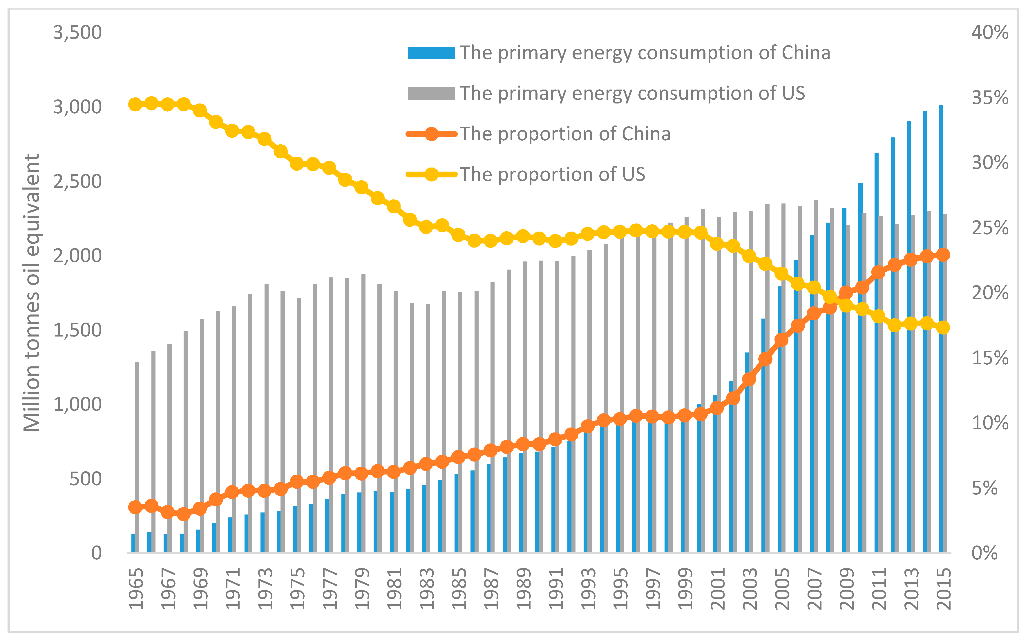
With the rapid economic growth since the beginning of the 21st century, China’s total primary energy consumption has been growing. In 2009, China surpassed the United States to become the world’s largest energy consumer; with primary energy consumption of 3014 million tons of oil equivalent (toe) in 2015, accounting for 22.92% of the world’s consumption. In comparison, the primary energy consumption of the United States has remained stable since the peak level of 2350 million toe in 2005. At the same time, the proportion US energy consumption has been experiencing a rapid decline since 2000. In 2015, the primary energy consumption of the USA was about 2280 million toe, accounting for 17.35% of global consumption (Figure 1).
China’s energy consumption is dominated by fossil fuels. Due to the rapidly growing energy consumption and fossil energy-based structure, the country’s carbon emissions have increased rapidly. According to [1], China’s CO2 emissions in 2015 totaled 9154 million tons, accounting for 27.3% of the world’s total emissions. With the growing concerns about global warming, China is facing enormous pressure on energy conservation and emission reduction.
According to the National Bureau of Statistics, the industrial sector can be divided into heavy and light industry according to production or living materials. The heavy industry is the main source of energy consumption and carbon emissions in China. Specifically, it includes the energy, steel, metallurgy, machinery, chemical, materials, and other industrial sectors which provide raw materials, fuel, power, technical equipment and other production materials for the economy [2]. Compared with the light industry, energy-intensity is one of the major features of heavy industry.
China’s energy consumption is concentrated in the heavy industry, which accounted for over 65% of the total energy consumption [3]. Since the founding of the People’s Republic of China (PRC), China has built a complete industrial system, but the different characteristics of the industrial sectors cause huge sectoral differences in energy consumption and energy intensity. It is necessary to make targeted energy saving and emissions reduction policies according to the industry characteristics.
In recent years, energy substitution is considered as one of the most important ways to solve the problems of resource constraints and environmental pressures, and also achieve sustainable development [4,5,6,7]. Energy substitution can be specifically divided into inter-fuel substitution and inter-factor substitution. Inter-fuel substitution is mainly about energy structure optimization, while inter-factor substitution is about the effective allocation of social resources, including energy, capital, labor and other input factors for production. Typically, by adjusting the proportion of other input factors on the basis of changes in the relative price of energy, the optimal marginal production of energy inputs can be achieved and perhaps realize the purpose of energy conservation [8]. As inter-fuel substitution is subject to certain factors like resource endowments, technology and total costs, people tend to focus more on inter-factor substitution between energy and other input factors [9,10].
The concept of substitution elasticity was first proposed by Hicks [11]. Hick’s substitution elasticity reflects the relative proportion of changes in input factors caused by the change in the marginal technical substitution rate. The shortcoming of Hick’s elasticity of substitution is that the estimation needs to be carried out based on the hypothesis that other input factors remain unchanged, which is obviously a biased estimation. Hick’s substitution elasticity was improved by [12], and then proven by [13], which has been named Allen elasticity of substitution (AES).
However, AES is also a kind of biased estimation, and some limitations cannot be addressed. For instance, AES cannot provide the relative proportion of two input factors, neither can it be explained by the marginal rate of substitution. Thus, AES cannot adequately explain the substitute relationship between one input factor and another.
In [14], the cross-price elasticity (CPE) was proposed, which reflects the change in another input factor when the price of one factor changes. However, CPE can only and simply describe the absolute replacement between factors, for example, the change in capital when energy price changes. That is, CPE cannot explain the effect of changes in relative proportion of input factors on the changes in relative price; even if the increase in energy prices lead to a reduction in the demand for capital investment, it does not mean that the relative amount of capital investment per unit of product to energy input per unit of product decreases, while capital investment per unit of product rise.
Morishima Alternative Elasticity (MES) proposed by [15] is a relative replacement rate that can be obtained by the integration of Hicks substitution elasticity and the replacement rate of two or more factors. Through the comparison of MES and CPE, it is possible to estimate not only the response of the proportion of two input factors to the change in relative price, but also the difference between substitution at the macro and the micro levels.
In the existing empirical research on energy economics, the constant elasticity of substitution (CES) function with the hypothesis of neutral technological progress is mostly used [16,17,18]. However, the impact of input factors on output is not only related to the change in input factors themselves, but also related to the technology progress of different input factors, which are often not the same. It is clear that CES cannot fully reflect the interaction and relationship between input factors. Therefore, earlier research studies on energy substitution were mostly carried out using the translog production function (TPF) method [19,20,21].
TPF is a kind of production function with variable elasticity. However, just like the CES, there is a problem when estimating the substitution relationship in the TPF. The TPF assumes that all the input factors in the production function are endogenous, which obviously leads to multicollinearity problem when estimating the coefficients with linear regression. As a result, there exists a deviation in the elasticity of substitution between energy and other factors [6,22,23,24,25].
Multicollinearity does not affect the unbiased and least variance property of the ordinary least squares (OLS) estimator (Gauss-Markov Theory). However, although the OLS estimator has the least variance in all the linear estimators, the absolute value of this variance is not necessarily small. In fact, we can find a biased estimator, which has a small deviation, but the accuracy can be higher than the unbiased OLS estimator.
Based on this principle, the ridge regression is a method that can solve the problem of multicollinearity through the introduction of a biased constant to obtain the estimator. In the case of multicollinearity problems, the joint distribution between two collinear coefficients is a ridge surface, each point on the surface corresponds to a residual sum of square (RSS); and the higher the point, the smaller the corresponding RSS. This means that the highest point on the ridge surface corresponds to the smallest RSS [26,27].
Ridge regression is essentially an improved least squares estimation method. By discarding the unbiasedness of the original least squares method, the estimator of the ridge regression method is more realistic and reliable, and the tolerance to morbid data is much stronger than in the OLS [28,29].
In summary, this paper studies the substitution between energy and other input factors in China’s heavy industry using a ridge regression method based on the translog production function. The relevant conclusions can provide a reference for the targeted energy saving and emission reduction policies. The remainder of this paper is organized as follows. Section 2 shows the methods used in this paper. Section 3 reports the data sources and processing. Section 4 concludes the estimation results and main conclusion. Section 5 presents some corresponding policy implications based on the empirical results, and the last section include the references used in this paper.
2. Methodology
2.1. Translog Production Function
The translog production function (TPF) was first proposed by [30]. A translog production function which contains two input factors is in the form of Equation (1):
TPF is a variable elasticity production function, which is easy to estimate and also inclusive. It is a simple linear model which can be directly estimated using the singular linear model estimation method. Inclusion means it can approximate any form of production function, for example, let , the production function in Equation (1) can change into Cobb-Douglas production. Also, let , it can change into common elasticity of substitution (CES) production function. Therefore, we can analyze the interaction between energy and other input factors as well as the differences in technological progress with the TPF.
Taking the added value of China’s heavy industry (Y) as the dependent variable, and energy consumption (E), capital stock (K), and labor input (L) as independent variables, we can build a TPF as follows:
The output elasticity is defined as the relative change in output caused by the relative change in input factor under the premise that technology and prices are constant. In Equation (2), the output elasticity of each input factor is:
The substitution elasticity is defined as the relative change in the proportion of input factors caused by a relative change in the marginal rate of substitution technology under the premise that the technology and prices are constant. On the basis of Equation (2), the substitution elasticity between different factors are as follows:
where , and represents the marginal output of capital, labor and energy, respectively. According to [31], we give the deduced procedure of as:
Further, we can obtain:
because:
Substituting Equations (12) and (13) into Equation (11) gives:
Also, by substituting Equation (14) into Equation (10), we can have:
Similarly, we can have the other two substitution elasticities as:
2.2. Ridge Regression
The basic linear regression model is in the form of Equation (18):
The OLS estimator of is:
Due to the interaction and squared terms of the input variables in Equation (2), the model is likely to suffer from severe multicollinearity, a statistical phenomenon in which two or more predictor variables in a multiple regression model are highly correlated, thereby violating a basic necessary condition for OLS to be unbiased. The coefficient estimates for the design matrix X have an approximate linear dependence, and Equation (19) becomes close to singular. As a result, the least squares estimate becomes highly sensitive to random errors in the observed response Y, producing a large variance. If there is multicollinearity between the independent variables, which is , then we can know that will increase, which is harmful for the parameter estimation. Adding a normal matrix to , where is the unit matrix, then the possibility of is lower than the possibility of , which can avoid the variance of increasing because of . The ridge regression estimator is:
where is the ridge regression estimator of , while is the ridge parameter or the biasing parameter which satisfies . , and I is the identity matrix. In general, there is an optimum value of . for any problem. However, it is desirable to examine the ridge solution for a range of admissible values of . Small positive values of improve the conditioning of the problem and reduce the variance of the estimates. While biased, the reduced variance of the ridge estimates usually results in a smaller mean square error when compared to least-squares estimates. In the econometric literature, several methods of obtaining the optimal value of the ridge parameter have been proposed. This study uses the ridge trace plot method which is the most popular in the literature. The coefficients are estimated with various levels of from zero to one. The coefficients are then plotted with respect to the values of and the optimal value is chosen at the point where the bi coefficients seem to stabilize.
3. Data
3.1. Capital Stock
In China, capital stock is not included in the official statistics, so we construct the capital stock of heavy industry using the perpetual inventory method [32].
where is the depreciate rate, and are the original value and net value of fixed assets in year t, respectively. is the accumulated depreciation in year t, and is the depreciation of year t. We then calculate the added amount of investment in year t as:
where represents the newly added investment in year t. Capital stock is calculated by the summing up the newly added investment in year t and the capital stock in year t − 1 minus depreciation. The capital stock in the prime year is the net value of fixed assets in 1980. All the asset values are converted into constant price in 1990 according to the price index of fixed asset investment from the China Economic Database.
The calculated capital stock of China’s heavy industry is shown in Figure 2:
3.2. Energy Consumption
The heavy industry contains a large number of sub-sectors, including energy production and storage sectors. To avoid double counting, we use the terminal energy consumption of each sub-sector to get the total energy input of the heavy industry.
According to the Organization for Economic Cooperation and Development (OECD) and International Energy Agency (IEA), terminal energy consumption refers to energy used by the terminal energy equipment. By this definition, we can infer that terminal energy consumption is equal to primary energy consumption minus the energy loss in processing, conversion and storage, as well as that which is lost in the production process of the energy industry. Losses in the intermediate process include loss in coal preparation and briquette, loss in oil refining, loss in oil and gas fields, power generation, power plant heating, coking, gas loss, transmission loss, loss in coal storage and transportation, and loss in oil and gas transportation. The terminal energy consumption of each sub-sector is from China energy Statistical Yearbook.
3.3. Output and Labor
The output of the heavy industry in this paper is represented by the added value, which is the newly added value in the production process of industrial enterprises. The sum of the added value of each sector is the gross domestic product, and labor is indicated by the number of employees. According to the definition of National Bureau of Statistics, China’s heavy industry includes 26 sub-sectors, covering all areas from mining to manufacturing and other industries. The added value and total employee of China’s heavy industry can be obtained by adding each sub-sector. The date on the added value and employee of each sub-sector are from China Industry Economy Statistical Yearbook and CEIC database, and it spans the years 1980 to 2014. This is because the energy consumption data of each sub-sector before 1980 and after 2014 is not available. If not specifically pointed out, all data are in 1990 constant prices according to the industrial producer price index (PPI) in order to eliminate the impact of inflation.
The statistics of the variables used in this paper are shown in Table 1:
4. Empirical Results
As mentioned above, there is a multicollinearity problem, which we believe might lead to an invalidation of the original least square (OLS) estimator. To prove the existence of multi-collinearity among the variables, Pearson’s correlation coefficients were computed and the results are shown in Table 2. By ranging between +1 and −1, the Pearson correlation coefficient can measure the dependence between two variables (+1 is total positive correlation, −1 is total negative correlation, and 0 is no correlation). The results show that there is a significant multi-collinearity among the variables, thus we use ridge regression instead of the OLS in this paper.
Sensitivity analysis shows that the results are not very sensitive to how the value of the ridge parameter is selected. For this reason, this paper relies on the ridge trace plot to determine the best value of K. Ridge trace plot showed the relationship between coefficients and K, which can fully reflect the effect of different value of K on the estimated value of coefficients. According to the variation in the values of the R-square and the coefficients of ridge regression for different values of K in Table 3, most values become steady when K approaches 0.30 and 0.40. When K is less than 0.30, the values of the coefficients are unstable, varying significantly with K. We can also see from the ridge trace in Figure 3 that when K is around 0.35, the ridge trace becomes steady. At the same time, Figure 4 shows that the R-Square falls rapidly when , and then begins to fall slightly when (the vertical line). Thus, the value of K is 0.35 in this paper.
The results of the ridge regression with is shown in Table 4. The relevant statistical tests show that the results of the ridge regression are significant. All the indicators of statistical testing, such as Adjusted R-Square, Standard Error (SE), significance level of regression equation (value of F and Sig F), as well as the ANOVA table, depict a reasonable model. More importantly, whether this model is good or not depends on the ability of the ridge regression to efficiently overcome the multicollinearity problem, and also the reasonableness of the estimated parameters. From Table 4 we can find that the statistical tests of the coefficients are ideal due to their rather small Standard Error (66.7%) which is smaller than 0.01, and is 0.10. Thus, the ridge regression estimators are reasonable.
According to the ridge regression estimators, Equation (2) can be rewritten as:
From the coefficients in Equation (24), the output elasticity of each input factor can be calculated according to Equations (3)–(5), while the elasticity of substitution between input factors can be calculated according to Equations (15) and (17). The results are shown in Table 5.
The output elasticity of energy, labor and capital have been increasing over the years (1980–2014), indicating that there is continuous overall technology progress. Among the three output elasticities, the elasticity of energy is the largest, followed by capital, and then labor (Figure 5). Though the output elasticity of labor is the smallest, the growth rate of the output elasticity of labor is the highest. During the period 1980–2014, the output elasticity of capital was 0.5115–0.6121 (an increase of 19.67%); the output elasticity of energy was 0.7969–0.9634 (an increase of 20.89%); and the output elasticity of labor was 0.1317–0.2044 (an increase of 55.20%).
The heavy industry is both energy- and capital-intensive. Notwithstanding this, some sub-sectors are labor-intensive, which is proved by the results of the estimated output elasticities. In general, the production of the heavy industry is highly dependent on energy and capital inputs, with the effect of labor inputs being relatively small. These are all determined by the characteristics of the heavy industry itself. On the other hand, in the period of the rapid development of the heavy industry, energy consumption and investment in fixed assets will grow rapidly.
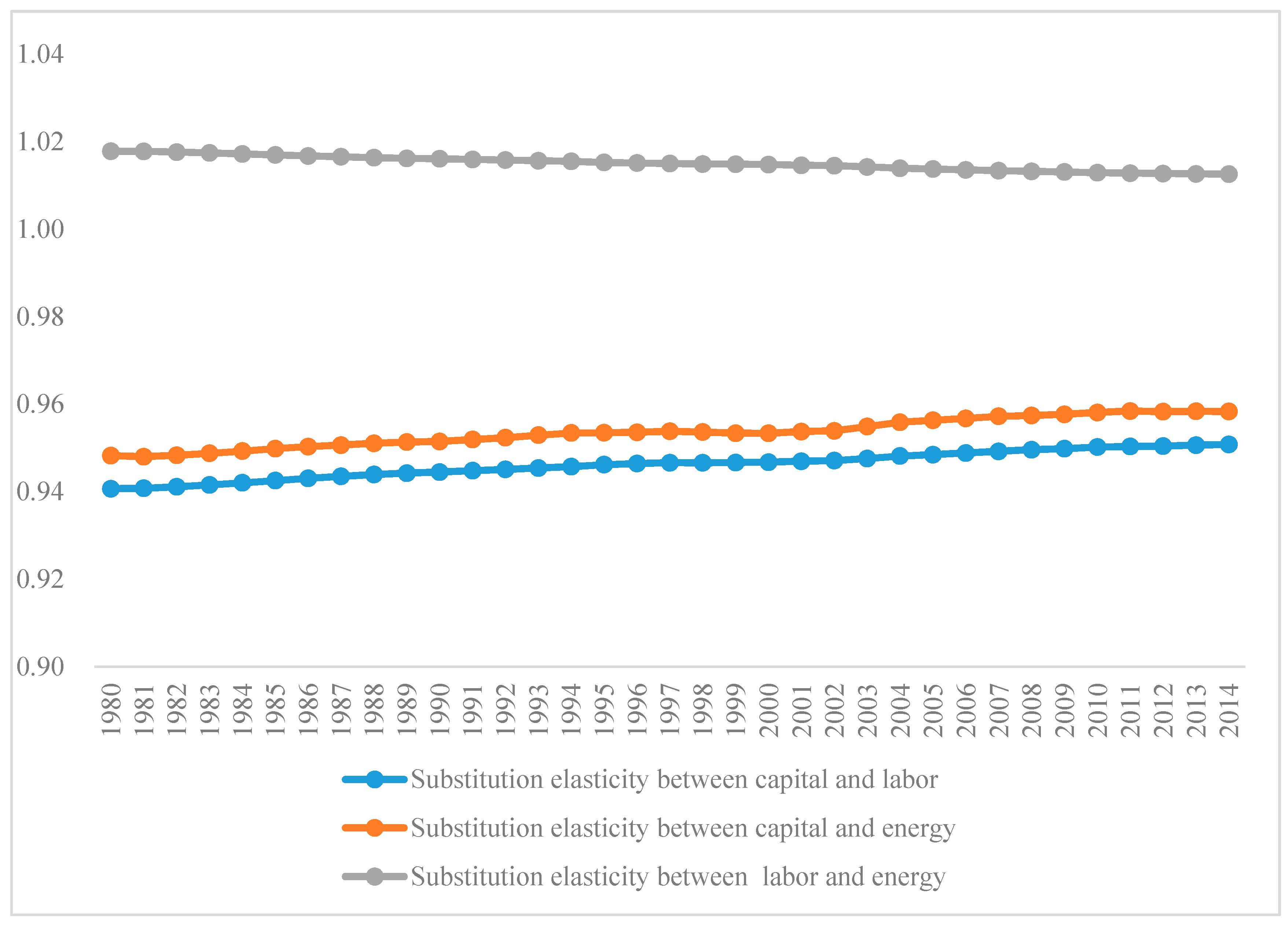
Then we look at the elasticity of substitution between the pair of capital, labor, and energy. From Figure 6, all the estimated elasticities of the heavy industry are positive. According to the definition in Equations (15)–(17), positive elasticity means that the relationship between capital and labor, capital and energy, labor and energy are substitute. On the other hand, the elasticity of substitution between capital and labor is almost the same with capital and energy. Both are in the interval of 0.94–0.96 during the period 1980–2014. The result indicates that the energy consumption and labor input of China’s heavy industry can be effectively saved by increasing the capital input.
The elasticity of substitution between labor and energy is relatively high, indicating that the substitution between labor and energy in the heavy industry is efficient. The substitution between labor and energy can be explained as follows: if a factory invests in more machines, more energy will be consumed, which may obviously decrease labor input. With the increasing popularity of automation equipment, energy and labor becomes more substitutable. In past years, especially after the 1990s, the price of labor inputs in China has been relatively low. Likewise, the existence of many migrant workers made labor supply sufficient. Factories in the heavy industry chose to use more labor inputs than capital and energy inputs. In this sense, China’s labor market has played a positive role in reducing energy consumption in the heavy industry. The effect of the substitute relationship between capital and energy is similar. More capital input can aid invest more efficient machines, which can reduce the energy consumption of a given output.
In recent years, with the increase of labor costs and population aging, China’s demographic bonus is gradually disappearing. This also explains the decreasing elasticity of substitution between labor and energy. With increasing resource constraints and environment pressures, future energy substitutes will mainly rely on the substitution of capital for energy and labor. The slightly upward trend in the substitution between capital and energy and labor suggests that the substitution is effective. The increasing trends of this substitution also indicate a bigger space for remitting energy supply shortage with more capital contribution.
In order to give an indication of the overall energy conservation and emission reduction effect of the substitution between capital and energy in China’s heavy industry, we estimate the energy saving and CO2 emission reduction potential in different scenarios. The results are shown in Table 6.
The average growth rate of capital stock for the past 30 years is 9.29%. If capital input increases by 10% in 2014 (ceteris paribus), it will lead to 131.64 million tons coal equivalent (Mtce) of energy conservation in China’s heavy industry, and 328.17 million tons of CO2 emission reduction (the carbon emission coefficient is assumed as 2.493 per ton). If the growth rate of capital input increases by 20%, the corresponding energy conservation and CO2 emission reduction will be 263.27 Mtce and 656.34 million tons, respectively.
5. Conclusions and Policy Implications
In this paper, a translog production function with input factors including energy, capital, and labor is established for China’s heavy industry. Using ridge regression, the output elasticity of each input factor and the elasticity of substitution between these input factors are analyzed. The main results are as follows.
Firstly, the output elasticity of energy, capital, and labor are all positive, which means that increase in factor inputs increases total output. Moreover, the level and growth rates of the output elasticities of all the three factors increased in the period 1980–2014, indicating that the efficiency of China’s heavy industry is improving. Despite this, the growth rates are rather moderate, indicating that the effect of increasing returns to scale in the heavy industry is wearing off. From the perspective of absolute value, the output elasticity of energy is the largest, followed by that of capital. The output elasticity of labor is the least, indicating that China’s heavy industry is both energy and capital-intensive, while the importance of labor is relatively less. The development of the heavy industry is highly correlated with macroeconomic environment. Thus, it will have an obvious impact on total energy consumption.
Secondly, the elasticities of substitution between energy, capital, and labor are all positive, indicating that all the three input factors are substitutes. The elasticity of substitution between labor and energy is relatively high (around 1.0178–1.0125 during 1980–2014), while the absolute value of the elasticity is decreasing. If industrial upgrading and improvement in the degree of automation continues, coupled with rising labor costs, the substitution effect of labor for energy in China’s heavy industry in the future will decline. The elasticities of substitution between capital and energy and labor are similar in terms of absolute value and trend. Capital and energy are substitutes in the heavy industry, and can be explained as follows: when an enterprise chooses to put more capital into improving energy efficiency, the energy consumption for a given output will decrease. However, it is worth noting that the operation of machinery will consume energy, and energy and capital may be complements, which is not conductive for energy conservation and emission reduction. For policy developments, the substitution between energy and capital depends on the direction of capital inputs, that is, energy saving or energy consumption. Government should encourage enterprises to invest in the improvement of energy efficiency through some fiscal and tax policies, and avoid extensive expansion of production capacity.
Thirdly, as China’s heavy industry accounts for over 60% of China’s total primary energy consumption, the substitution effect will bring about huge energy conservation and emission reduction. The existence of a substitution relationship indicates that the energy consumption constraints the heavy industry is facing can be improved by increasing capital input. With more investment, energy-efficient technology could be applied, and this can promote the substitution between capital and energy. The substitution relationship between capital and labor is similar. On the other hand, the elasticity of substitution is increasing, indicating that there is a chance of reducing the energy constraints when the heavy industry is more capital-intensive.
In summary, China’s heavy industry is both energy- and capital-intensive. More capital input can help improve energy efficiency, which will eventually help accomplish the goal of energy conservation. As capital is substituted for energy and labor, more capital inputs are used in China’s heavy industry from the perspective of energy conservation and emission reduction. It is important to understand the substitution relationship between energy and other input factors to improve the quality of development of China’s heavy industry and also optimize its development model. It is worth noting that there is need to differentiate between advanced and backward production capacity in some energy-intensive sectors in China’s heavy industry. The former can be promoted through some pricing policies like carbon tax, while the latter can be addressed by some administrative means in order to achieve a rapid effect.
Acknowledgments
The paper is supported by the Grant for Collaborative Innovation Center for Energy Economics and Energy Policy (No. 1260-Z0210011), Xiamen University Flourish Plan Special Funding (No. 1260-Y07200) and China National Social Science Fund (No. 15ZD058).
Author Contributions
Kui Liu and Boqiang Lin conceived, designed, prepared and revised the paper. Kui Liu and Boqiang Lin approved the final manuscript.
Conflicts of Interest
The authors declare no conflict of interest.
References
- The British Petroleum Company. BP Statistical Review of World Energy 2016. Available online: https://www.bp.com/en/global/corporate/energy-economics/statistical-review-of-world-energy/downloads.html (accessed on 14 October 2017).
- Lin, B.; Liu, K. How Efficient Is China’s Heavy Industry? A Perspective of Input–Output Analysis. Emerg. Mark. Financ. Trade 2016, 52, 2546–2564. [Google Scholar] [CrossRef]
- Lin, B.; Li, J. The rebound effect for heavy industry: Empirical evidence from China. Energy Policy 2014, 74, 589–599. [Google Scholar] [CrossRef]
- Field, B.C.; Grebenstein, C. Capital-energy substitution in US manufacturing. Rev. Econ. Stat. 1980, 62, 207–212. [Google Scholar] [CrossRef]
- Koetse, M.J.; de Groot, H.L.; Florax, R.J. Capital-energy substitution and shifts in factor demand: A meta-analysis. Energy Econ. 2008, 30, 2236–2251. [Google Scholar] [CrossRef]
- Chang, K.-P. Capital-energy substitution and the multi-level CES production function. Energy Econ. 1994, 16, 22–26. [Google Scholar] [CrossRef]
- Prywes, M. A nested CES approach to capital-energy substitution. Energy Econ. 1986, 8, 22–28. [Google Scholar] [CrossRef]
- Lin, B.; Fei, R. Analyzing inter-factor substitution and technical progress in the Chinese agricultural sector. Eur. J. Agron. 2015, 66, 54–61. [Google Scholar] [CrossRef]
- Welsch, H.; Ochsen, C. The determinants of aggregate energy use in West Germany: Factor substitution, technological change, and trade. Energy Econ. 2005, 27, 93–111. [Google Scholar] [CrossRef]
- Wang, X.; Lin, B. Factor and fuel substitution in China’s iron & steel industry: Evidence and policy implications. J. Clean. Prod. 2017, 141, 751–759. [Google Scholar]
- Hicks, J.R. Marginal productivity and the principle of variation. Economica 1932, 35, 79–88. [Google Scholar] [CrossRef]
- Hicks, J.R.; Allen, R.G. A reconsideration of the theory of value. Part I. Economica 1934, 1, 52–76. [Google Scholar] [CrossRef]
- Uzawa, H. Production functions with constant elasticities of substitution. Rev. Econ. Stud. 1962, 29, 291–299. [Google Scholar] [CrossRef]
- Allen, R.G.D. Mathematical Analysis for Economists; St. Martin’s Press: New York, NY, USA, 1938. [Google Scholar]
- Morishima, M. A few suggestions on the theory of elasticity. Keizai Hyoron (Econ. Rev.) 1967, 16, 144–150. [Google Scholar]
- Özatalay, S.; Grubaugh, S.; Long, T.V. Energy substitution and national energy policy. Am. Econ. Rev. 1979, 69, 369–371. [Google Scholar]
- Pindyck, R.S. Interfuel substitution and the industrial demand for energy: An international comparison. Rev. Econ. Stat. 1979, 169–179. [Google Scholar] [CrossRef]
- Sato, K. A two-level constant-elasticity-of-substitution production function. Rev. Econ. Stat. 1967, 34, 201–218. [Google Scholar] [CrossRef]
- Smyth, R.; Narayan, P.K.; Shi, H. Inter-fuel substitution in the Chinese iron and steel sector. Int. J. Prod. Econ. 2012, 139, 525–532. [Google Scholar] [CrossRef]
- Ma, H.Y.; Oxley, L.; Gibson, J.; Kim, B. China’s energy economy: Technical change, factor demand and interfactor/interfuel substitution. Energy Econ. 2008, 30, 2167–2183. [Google Scholar] [CrossRef]
- Lin, B.; Xie, C. Energy substitution effect on transport industry of China-based on trans-log production function. Energy 2014, 67, 213–222. [Google Scholar] [CrossRef]
- Griffin, J.M.; Gregory, P.R. An intercountry translog model of energy substitution responses. Am. Econ. Rev. 1976, 66, 845–857. [Google Scholar]
- Kim, H.Y. The translog production function and variable returns to scale. Rev. Econ. Stat. 1992, 74, 546–552. [Google Scholar] [CrossRef]
- Berndt, E.R.; Christensen, L.R. The translog function and the substitution of equipment, structures, and labor in US manufacturing 1919–68. J. Econom. 1973, 1, 81–113. [Google Scholar] [CrossRef]
- Zheng, Z.-N.; Liu, D.-S. China’s Trans-log Production Function Using Capital, Energy and Labor as Input. Syst. Eng. Theory Pract. 2004, 5, 51–54. [Google Scholar]
- Hoerl, A.E. Application of ridge analysis to regression problems. Chem. Eng. Prog. 1962, 58, 54–59. [Google Scholar]
- Tikhonov, A. Solution of Incorrectly Formulated Problems and the Regularization Method. Soviet Math. Dokl. 1963, 5, 1035–1038. [Google Scholar]
- Hoerl, A.E.; Kennard, R.W. Ridge regression: Biased estimation for nonorthogonal problems. Technometrics 1970, 12, 55–67. [Google Scholar] [CrossRef]
- Hoerl, A.E.; Kennard, R.W. Ridge regression: Applications to nonorthogonal problems. Technometrics 1970, 12, 69–82. [Google Scholar] [CrossRef]
- Christensen, L.R.; Jorgenson, D.W.; Lau, L.J. Transcendental logarithmic production frontiers. Rev. Econ. Stat. 1973, 55, 28–45. [Google Scholar] [CrossRef]
- Xie, C.P.; Hawkes, A.D. Estimation of inter-fuel substitution possibilities in China’s transport industry using ridge regression. Energy 2015, 88, 260–267. [Google Scholar] [CrossRef]
- Chen, S. Reconstruction of sub-industrial statistical data in China (1980–2008). China Econ. Q. 2011, 10, 735–776. [Google Scholar]
Figure 1.
The primary energy consumption of China and US and their proportions to the world.

Figure 2.
The capital stock of China’s heavy industry in 1980–2014.
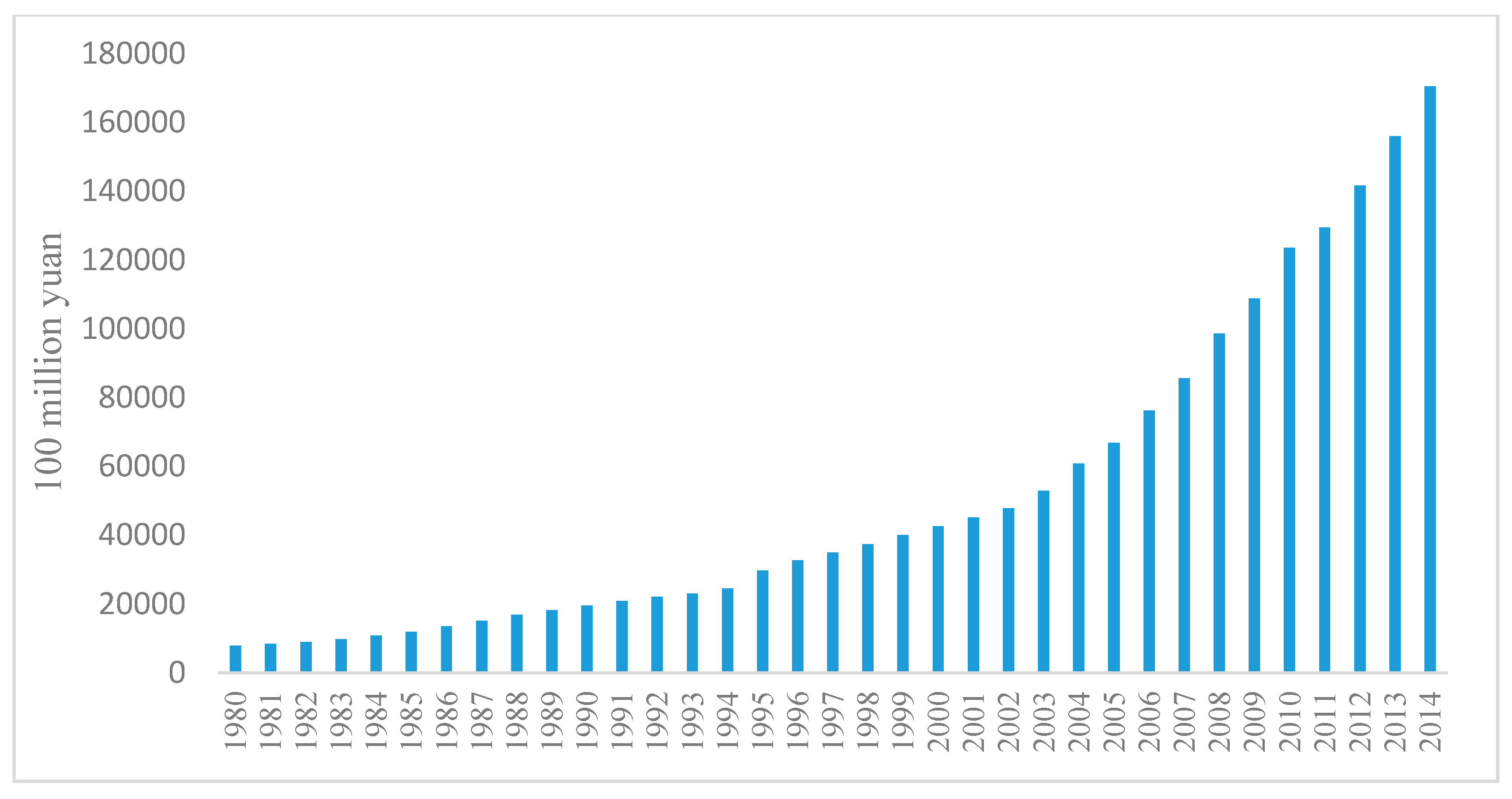
Figure 3.
Ridge trace of the coefficient estimates of the ridge regression.
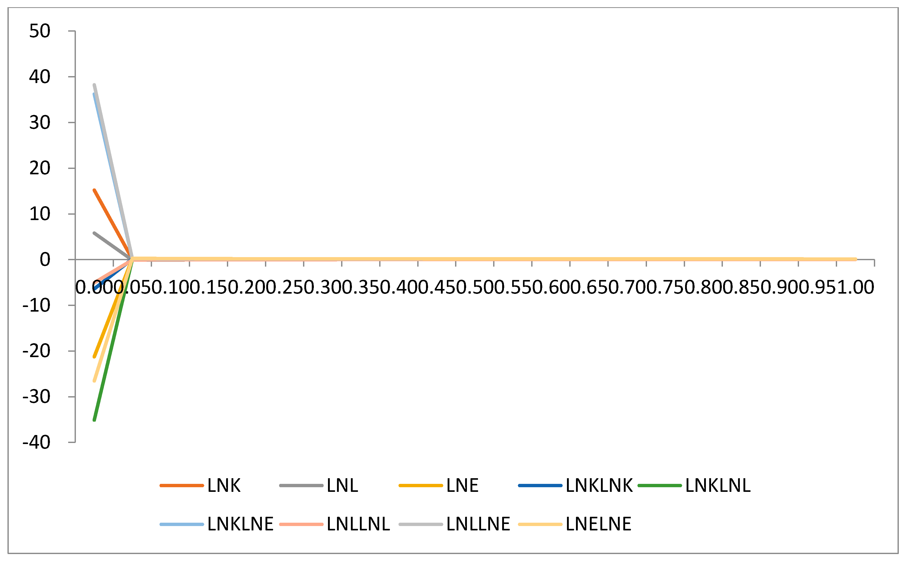
Figure 4.
The scatterplot between R-square and K.
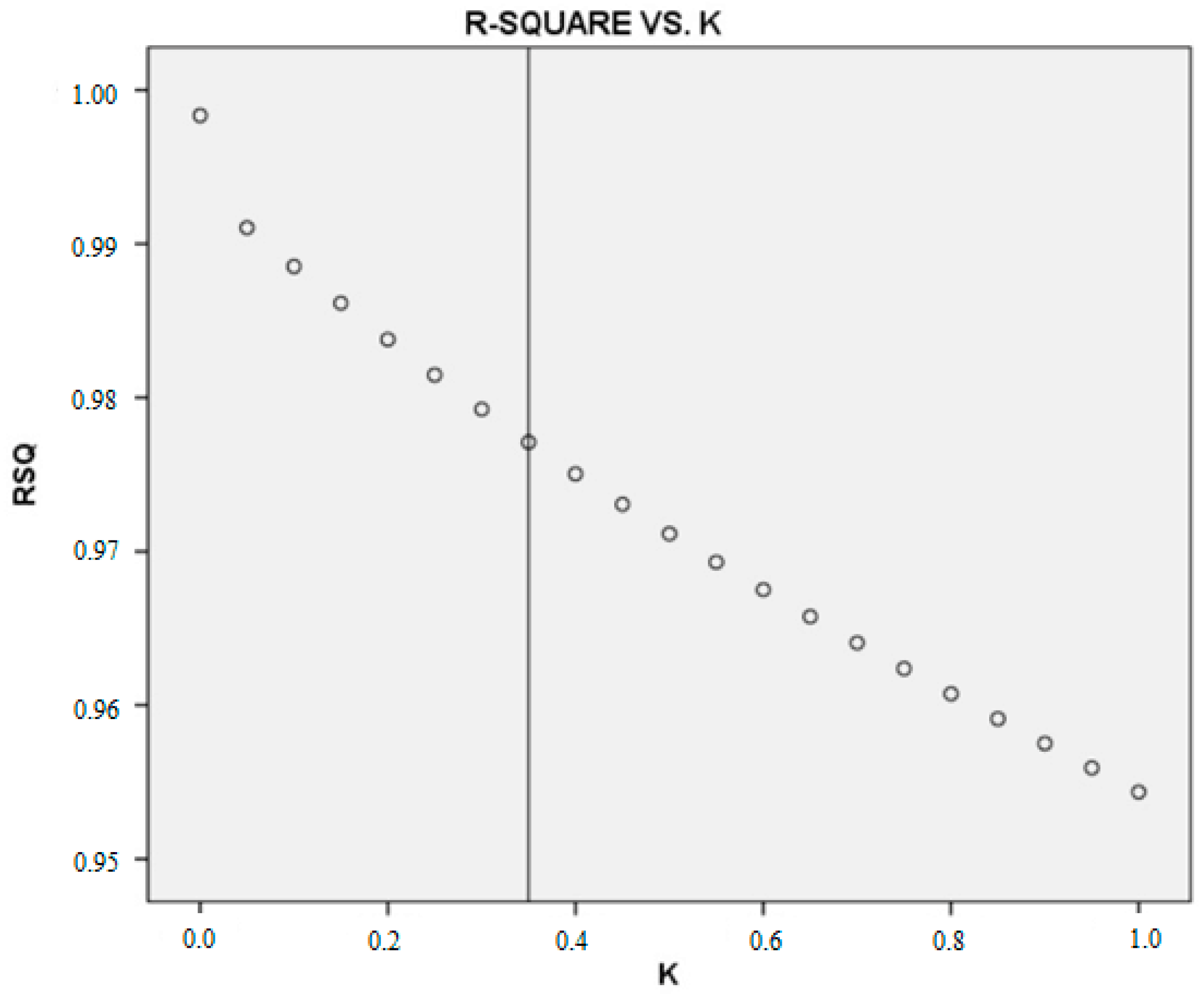
Figure 5.
The output elasticity of capital, labor and energy.
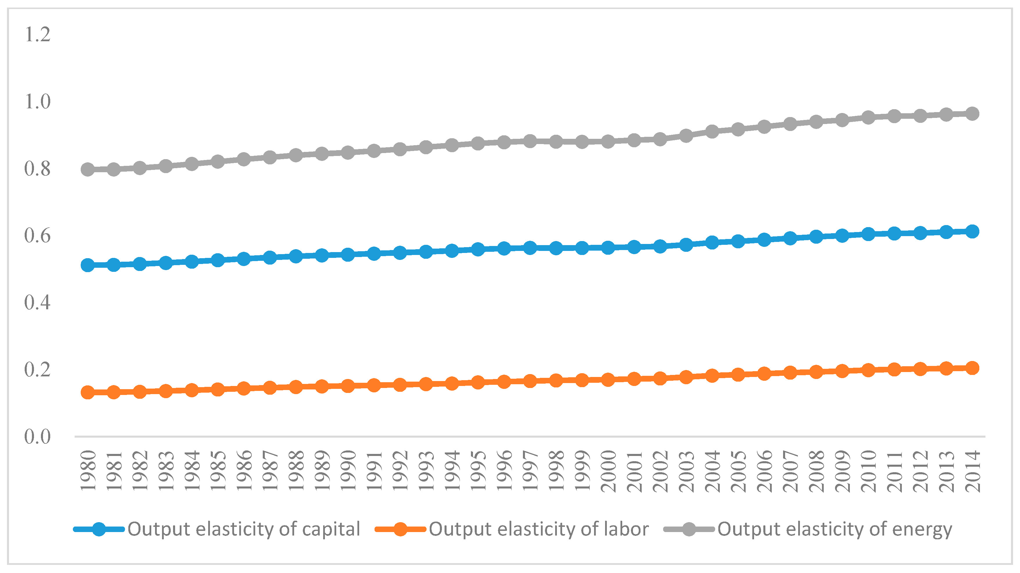
Figure 6.
The substitution elasticity between capital, labor, and energy.


Table 1.
Statistics of variables used in this paper.
| Variable | Obs | Mean | Std. Dev. | Min | Max |
|---|---|---|---|---|---|
| Output | 35 | 25,751.01 | 31,423.81 | 2399.00 | 106,109.70 |
| Capital | 35 | 51,790.68 | 46,530.36 | 7916.28 | 170,377.80 |
| Labor | 35 | 4676.70 | 1427.98 | 2386.01 | 7195.62 |
| Energy | 35 | 579.06 | 393.17 | 166.00 | 1373.64 |
Table 2.
Correlation analysis of variables.
| Output | Capital | Labor | Energy | ||
|---|---|---|---|---|---|
| Output | Pearson Correlation | 1 | 0.991 ** | 0.827 ** | 0.976 ** |
| Sig. (2-tailed) | -- | 0 | 0 | 0 | |
| N | 35 | 35 | 35 | 35 | |
| Capital | Pearson Correlation | 0.991 ** | 1 | 0.854 ** | 0.989 ** |
| Sig. (2-tailed) | 0 | -- | 0 | 0 | |
| N | 35 | 35 | 35 | 35 | |
| Labor | Pearson Correlation | 0.827 ** | 0.854 ** | 1 | 0.874 ** |
| Sig. (2-tailed) | 0 | 0 | -- | 0 | |
| N | 35 | 35 | 35 | 35 | |
| Energy | Pearson Correlation | 0.976 ** | 0.989 ** | 0.874 ** | 1 |
| Sig. (2-tailed) | 0 | 0 | 0 | -- | |
| N | 35 | 35 | 35 | 35 |
** means correlation is significant at the 0.01 level (2-tailed).
Table 3.
R-square and beta coefficients for estimated values of K.
| K | RSQ | LNK | LNL | LNE | LNKLNK | LNKLNL | LNKLNE | LNLLNL | LNLLNE | LNELNE |
|---|---|---|---|---|---|---|---|---|---|---|
| 0.00 | 0.9984 | 15.1871 | 5.7819 | −21.2592 | −6.4124 | −35.1092 | 36.2057 | −5.0518 | 38.2264 | −26.5467 |
| 0.05 | 0.9911 | 0.0983 | −0.1029 | 0.1913 | 0.1529 | 0.0765 | 0.2100 | −0.0784 | 0.1581 | 0.2573 |
| 0.10 | 0.9885 | 0.1282 | −0.0760 | 0.1773 | 0.1594 | 0.0905 | 0.1898 | −0.0620 | 0.1379 | 0.2150 |
| 0.15 | 0.9862 | 0.1354 | −0.0570 | 0.1683 | 0.1579 | 0.0955 | 0.1784 | −0.0470 | 0.1298 | 0.1953 |
| 0.20 | 0.9838 | 0.1370 | −0.0423 | 0.1615 | 0.1548 | 0.0980 | 0.1701 | −0.0343 | 0.1251 | 0.1828 |
| 0.25 | 0.9815 | 0.1365 | −0.0303 | 0.1560 | 0.1514 | 0.0993 | 0.1636 | −0.0236 | 0.1219 | 0.1737 |
| 0.30 | 0.9792 | 0.1353 | −0.0204 | 0.1514 | 0.1481 | 0.1001 | 0.1583 | −0.0146 | 0.1195 | 0.1666 |
| 0.35 | 0.9771 | 0.1338 | −0.0120 | 0.1474 | 0.1451 | 0.1005 | 0.1537 | −0.0069 | 0.1176 | 0.1608 |
| 0.40 | 0.9750 | 0.1321 | −0.0049 | 0.1440 | 0.1422 | 0.1007 | 0.1498 | −0.0003 | 0.1160 | 0.1560 |
| 0.45 | 0.9731 | 0.1305 | 0.0012 | 0.1409 | 0.1396 | 0.1007 | 0.1463 | 0.0054 | 0.1145 | 0.1518 |
| 0.50 | 0.9712 | 0.1289 | 0.0066 | 0.1382 | 0.1372 | 0.1007 | 0.1432 | 0.0104 | 0.1133 | 0.1481 |
| 0.55 | 0.9693 | 0.1273 | 0.0113 | 0.1357 | 0.1350 | 0.1005 | 0.1404 | 0.0148 | 0.1122 | 0.1448 |
| 0.60 | 0.9675 | 0.1258 | 0.0154 | 0.1335 | 0.1329 | 0.1003 | 0.1379 | 0.0187 | 0.1111 | 0.1419 |
| 0.65 | 0.9658 | 0.1243 | 0.0191 | 0.1314 | 0.1310 | 0.1001 | 0.1356 | 0.0221 | 0.1101 | 0.1393 |
| 0.70 | 0.9641 | 0.1229 | 0.0223 | 0.1295 | 0.1292 | 0.0998 | 0.1334 | 0.0252 | 0.1092 | 0.1369 |
| 0.75 | 0.9624 | 0.1216 | 0.0252 | 0.1277 | 0.1275 | 0.0995 | 0.1315 | 0.0280 | 0.1083 | 0.1346 |
| 0.80 | 0.9607 | 0.1203 | 0.0279 | 0.1260 | 0.1259 | 0.0991 | 0.1296 | 0.0304 | 0.1075 | 0.1326 |
| 0.85 | 0.9591 | 0.1191 | 0.0302 | 0.1245 | 0.1244 | 0.0988 | 0.1279 | 0.0327 | 0.1067 | 0.1307 |
| 0.90 | 0.9575 | 0.1180 | 0.0323 | 0.1230 | 0.1230 | 0.0984 | 0.1263 | 0.0347 | 0.1060 | 0.1289 |
| 0.95 | 0.9559 | 0.1168 | 0.0343 | 0.1216 | 0.1216 | 0.0981 | 0.1247 | 0.0365 | 0.1052 | 0.1272 |
| 1.00 | 0.9544 | 0.1158 | 0.0360 | 0.1203 | 0.1203 | 0.0977 | 0.1233 | 0.0382 | 0.1045 | 0.1256 |
Table 4.
Model results of ridge regression.
| Ridge Regression with K = 0.35 | ||||
| R-Square | 0.97710 | |||
| Adjusted R-square | 0.96886 | |||
| Standard Error (SE) | 0.21830 | |||
| ANOVA Table | ||||
| Degree of Freedom (DF) | Stdev Squre (SS) | Mean Squre (MS) | ||
| Regress | 9 | 50.833 | 5.648 | |
| Residual | 25 | 1.191 | 0.048 | |
| F value | Sig F | |||
| 118.52448 | 0 | |||
| Variables in the Equation | ||||
| B | SE(B) | Beta | B/SE(B) | |
| 0.17954 | 0.01101 | 0.13378 | 16.31419 | |
| −0.04644 | 0.06161 | −0.01204 | −0.75379 | |
| 0.26951 | 0.01293 | 0.14741 | 20.84683 | |
| 0.00926 | 0.00050 | 0.14507 | 18.48060 | |
| 0.01152 | 0.00048 | 0.10051 | 24.03356 | |
| 0.01483 | 0.00068 | 0.15373 | 21.76466 | |
| −0.00160 | 0.00364 | −0.00694 | −0.44023 | |
| 0.01945 | 0.00072 | 0.11758 | 27.06722 | |
| 0.02370 | 0.00119 | 0.16084 | 19.95578 | |
| Constant | 1.48061 | 0.62412 | 0.00000 | 2.37231 |
The values of “B” represent coefficients for corresponding variables, and values of “SE(B)” represent the corresponding standard error of each coefficient.
Table 5.
Output and substitution elasticities of each input factor.
| Year | ||||||
|---|---|---|---|---|---|---|
| 1980 | 0.5115 | 0.1317 | 0.7969 | 0.9406 | 0.9482 | 1.0178 |
| 1981 | 0.5123 | 0.1322 | 0.7971 | 0.9407 | 0.9480 | 1.0177 |
| 1982 | 0.5148 | 0.1337 | 0.8012 | 0.9411 | 0.9483 | 1.0176 |
| 1983 | 0.5181 | 0.1358 | 0.8069 | 0.9415 | 0.9487 | 1.0174 |
| 1984 | 0.5220 | 0.1381 | 0.8134 | 0.9420 | 0.9493 | 1.0172 |
| 1985 | 0.5260 | 0.1406 | 0.8204 | 0.9425 | 0.9498 | 1.0169 |
| 1986 | 0.5303 | 0.1433 | 0.8274 | 0.9430 | 0.9503 | 1.0167 |
| 1987 | 0.5340 | 0.1456 | 0.8332 | 0.9435 | 0.9506 | 1.0165 |
| 1988 | 0.5378 | 0.1479 | 0.8394 | 0.9439 | 0.9510 | 1.0163 |
| 1989 | 0.5405 | 0.1496 | 0.8438 | 0.9442 | 0.9513 | 1.0162 |
| 1990 | 0.5428 | 0.1510 | 0.8472 | 0.9445 | 0.9515 | 1.0161 |
| 1991 | 0.5457 | 0.1528 | 0.8525 | 0.9448 | 0.9519 | 1.0159 |
| 1992 | 0.5484 | 0.1545 | 0.8575 | 0.9451 | 0.9523 | 1.0158 |
| 1993 | 0.5513 | 0.1563 | 0.8634 | 0.9454 | 0.9529 | 1.0156 |
| 1994 | 0.5543 | 0.1582 | 0.8693 | 0.9457 | 0.9534 | 1.0155 |
| 1995 | 0.5586 | 0.1617 | 0.8747 | 0.9461 | 0.9534 | 1.0152 |
| 1996 | 0.5612 | 0.1635 | 0.8783 | 0.9464 | 0.9535 | 1.0151 |
| 1997 | 0.5629 | 0.1655 | 0.8814 | 0.9466 | 0.9538 | 1.0150 |
| 1998 | 0.5623 | 0.1675 | 0.8799 | 0.9466 | 0.9536 | 1.0149 |
| 1999 | 0.5627 | 0.1683 | 0.8793 | 0.9466 | 0.9533 | 1.0148 |
| 2000 | 0.5636 | 0.1696 | 0.8803 | 0.9467 | 0.9533 | 1.0147 |
| 2001 | 0.5655 | 0.1719 | 0.8844 | 0.9469 | 0.9537 | 1.0146 |
| 2002 | 0.5672 | 0.1733 | 0.8871 | 0.9471 | 0.9539 | 1.0145 |
| 2003 | 0.5723 | 0.1775 | 0.8977 | 0.9475 | 0.9549 | 1.0142 |
| 2004 | 0.5789 | 0.1818 | 0.9103 | 0.9481 | 0.9558 | 1.0139 |
| 2005 | 0.5825 | 0.1846 | 0.9168 | 0.9484 | 0.9563 | 1.0137 |
| 2006 | 0.5871 | 0.1877 | 0.9245 | 0.9488 | 0.9567 | 1.0135 |
| 2007 | 0.5916 | 0.1907 | 0.9325 | 0.9492 | 0.9572 | 1.0133 |
| 2008 | 0.5964 | 0.1928 | 0.9393 | 0.9496 | 0.9574 | 1.0132 |
| 2009 | 0.5994 | 0.1953 | 0.9443 | 0.9498 | 0.9577 | 1.0130 |
| 2010 | 0.6041 | 0.1982 | 0.9522 | 0.9502 | 0.9581 | 1.0129 |
| 2011 | 0.6059 | 0.2003 | 0.9561 | 0.9503 | 0.9584 | 1.0128 |
| 2012 | 0.6072 | 0.2016 | 0.9570 | 0.9504 | 0.9583 | 1.0127 |
| 2013 | 0.6101 | 0.2032 | 0.9611 | 0.9506 | 0.9583 | 1.0126 |
| 2014 | 0.6121 | 0.2044 | 0.9634 | 0.9508 | 0.9583 | 1.0125 |
Table 6.
Energy conservation and CO2 emission reduction of China’s heavy industry under different substitution scenarios in 2014. Million Tons Coal Equivalent (Mtce).
Table 6.
Energy conservation and CO2 emission reduction of China’s heavy industry under different substitution scenarios in 2014. Million Tons Coal Equivalent (Mtce).
| Year | Capital Input Increases by 10% | Capital Input Increases by 20% | ||
|---|---|---|---|---|
| Energy Conservation | Carbon Emission Reduction | Energy Conservation | Carbon Emission Reduction | |
| 2014 | 131.64 Mtce | 328.17 million tons | 263.27 Mtce | 656.34 million tons |
© 2017 by the authors. Licensee MDPI, Basel, Switzerland. This article is an open access article distributed under the terms and conditions of the Creative Commons Attribution (CC BY) license (http://creativecommons.org/licenses/by/4.0/).
Share and Cite
MDPI and ACS Style
Lin, B.; Liu, K. Energy Substitution Effect on China’s Heavy Industry: Perspectives of a Translog Production Function and Ridge Regression. Sustainability 2017, 9, 1892. https://doi.org/10.3390/su9111892
AMA Style
Lin B, Liu K. Energy Substitution Effect on China’s Heavy Industry: Perspectives of a Translog Production Function and Ridge Regression. Sustainability. 2017; 9(11):1892. https://doi.org/10.3390/su9111892
Chicago/Turabian StyleLin, Boqiang, and Kui Liu. 2017. "Energy Substitution Effect on China’s Heavy Industry: Perspectives of a Translog Production Function and Ridge Regression" Sustainability 9, no. 11: 1892. https://doi.org/10.3390/su9111892
Note that from the first issue of 2016, this journal uses article numbers instead of page numbers. See further details here.