Influencing Mechanism of Potential Factors on Passengers’ Long-Distance Travel Mode Choices Based on Structural Equation Modeling


MOE Key Laboratory for Urban Transportation Complex System Theory and Technology, School of Traffic and Transportation, Beijing Jiaotong University, Beijing 100044, China
*
Author to whom correspondence should be addressed.
Sustainability 2017, 9(11), 1943; https://doi.org/10.3390/su9111943
Submission received: 15 August 2017
/
Revised: 19 October 2017
/
Accepted: 23 October 2017
/
Published: 26 October 2017
Abstract
:Understanding the public transportation users’ preferences to long-distance travel modes would contribute to reasonable developing policies and resource allocation. This paper aims to explore the influencing mechanism of potential factors on the long-distance travel mode choice. A survey was conducted to collect the data. The analysis of variance (ANOVA) approach was applied to analyze the correlation relationship between potential factors and travel mode choice behavior. The results showed that, except gender, service demand for safety and departure time, all of the other factors significantly influenced the travel mode choice behavior. Specifically, passengers with higher education level and income level were more likely to choose high-speed railway (HSR) and plane; passengers caring about travel expense were more likely to choose ordinary train, whereas plane and HSR may be chosen more by passengers caring more about comfort, punctuality and efficiency; the more passengers were satisfied with travel modes’ service performance, the more they would be likely to choose them; the most competitive distance ranges for coach, ordinary train, HSR and plane were below 500 km, 500–1000 km, 500–1500 km and over 1500 km, respectively. Besides, the structural equation modeling (SEM) technique was applied to investigate the influencing mechanism of factors on the long-distance travel mode choice. The results revealed that travel distance was the most significant variable directly influencing passengers’ mode choices, followed by the service demand, performance evaluation, and personal attributes. Furthermore, personal attributes were verified to have an indirect effect on travel mode choice behavior by significantly affecting the service demand and performance evaluation.
1. Introduction
During the past two decades, China has been in a period of rapid urban development, with the rate of development increasing from 26.94% to 57.35% between 1991 and 2016 [1]. With the trend of rapid urbanization, China has seen a sharp growth in its long-distance multimode transportation system, including airlines, railways, and highways. On average, the annual increases of the modes’ mileages are 13.3% for airways, 4.5% for railway and 3.2% for highways. The most impressive achievement is the establishment of high-speed rail (HSR) system which is acknowledged widely as low-energy, high-capacity and high-efficiency. As of 2016, China had the world’s longest HSR network, with about 22,000 km in service [1]. Furthermore, there are plans to increase the HSR network to 30,000 km by 2020, based on a network of four vertical and four horizontal trunk lines.
With the huge growth in the usage of HSR, researchers found that passenger’s long-distance travel mode choice has significantly changed due to the diversification of alternative travel modes. Especially, the rapid rise of HSR has a huge impact on the traditional transportation modes and brings competitions [2] For example, after 48 days operation of HSR, all the flights between Xi’an and Zhengzhou (505 km) were cancelled by the airlines because of the low demand; after one year HSR operation, the number of flights between Wuhan and Guangzhou was reduced from 15 to 9, even though the distance is 1069 km [3]. With the concurrent improvement of Chinese social economy and income level, the passenger volume, travel distance, and trip frequency of the long-distance transportation have also been also rapidly increasing during the past two decades. Because HSR brings new development opportunities to the Chinese passenger transport market, there is an urgent need to better understand the characteristics of passengers’ long-distance travel behavior, which is influenced by various factors.
Many countries, including USA, Germany, UK, Spain and Korea et al. [4,5,6,7,8,9], have made great efforts to explore and understand passengers’ travel behavior in long-distance. Country-wide or city-wide travel surveys are conducted in these counties to measure the travel behavior characteristics. However, travel surveys in China mainly focus on investigating the passengers’ inner-city travel behavior, such as the Fourth Comprehensive Travel Surveys in Shanghai (2009) and Beijing (2010). The research findings in the previous studies cannot be applied to the long-distance travel behavior in China directly. On the one hand, the network structure of long-distance transportation modes is quite different between China and other countries, which will lead to great differences in passengers’ travel mode choice. Generally speaking, China strives to develop railway and Occident has advanced aviation system. On the other hand, the behavior features of long-distance travel are quite different from those of inner-city travel due to some important distinctions. Firstly, long-distance travel generally involves more time and expense, so passengers facing the mode choice decision are in a different situation compared with a short-distance travel [8]. Secondly, alternative travel modes are quite different. Available modes for long-distance travel mainly include ordinary train, high-speed railway, plane and coach, while, for inner-city, include urban rail transit, bus, bike, and car, and walk. Thirdly, there are obvious differences between the long-distance travel and inner-city travel in terms of travel distance and travel purpose. The principal motive of inner-city travel is commuting, while long-distance travel is mainly dominated by pleasure and business pursuits, which will cause differentiated service demands [10]. Thus, research on travel mode choice behavior in long-distance calls for special attention. Therefore, given the lack of literature, it is critical to focus on Chinese passengers’ travel mode choice among the different public transportation modes typically including HSR, ordinary train, plane and coach.
The motivation for this study is twofold. Firstly, we want to confirm whether the potential influencing factors significantly affect passengers’ travel mode choice behavior in long-distance travel. Secondly, this paper seeks to determine the influence degree of influencing factors and their interaction relationship. To do so, a survey was conducted to collect data providing a rich source of information on passenger travel mode choice behavior. The analysis of variance (ANOVA) approach is applied to detect whether the potential influencing factors have significant impact on passengers’ travel mode choice behavior. To better understand how these factors work, two hypotheses regarding the passenger travel mode choice behavior are proposed, and verified using SEM.
The paper is organized as follows. Section 2 reviews the related literature. Section 3 describes the survey design and the collected data structure. Section 4 presents the descriptive analyses of survey results. In Section 5, SEM method is applied to verify the hypotheses of passengers’ travel mode choice behavior characteristics. Finally, Section 6 provides concluding remarks.
2. Literature Review
2.1. Travel Behavior Investigation Literature Review
Extensive studies have been carried out to explore what factors significantly affect travel behavior, including passengers’ personal attributes such as vocation and income [7,11,12,13] education level [14]; trip attributes such as travel distance [15] and departure time [16,17]; and perception on different modes [18].
Passengers’ personal attributes are some of the key factors affecting travel mode choice behavior. Yu [19] found that travel behavior and activity patterns differ between age groups. The results showed that for the elderly, safety and convenience were the two most significant aspects in travel mode choice. Paulley et al. [20] and Santos et al. [14] explored the effects of passengers’ incomes and education levels on the demand for public transport, and found that both of them positively affected the transport mode share patterns. Georggi and Pendyala [12] indicated that groups with lower incomes were more likely to choose coach than those with higher incomes; with an increase in income level, the share of air travel increased steadily. Mallett [13] noted that although coach and trains were the two most important travel modes for the low-income groups, they still rarely chose those two modes for long-distance travel. The author also found that air travel accounted for about twice the share of the combination of coach and train trips for low-income groups.
Trip attributes such as departure time and travel distance significantly impact on choice behavior. Abdel-Aty and Jovanis [17] found that departure time had a significant impact on the travel behavior of the elderly. They reported that the elderly always avoided travelling at night or during the rush hour. Previous research has found that, for different travel distances, none of the modes can always have advantages over the others, and different travel modes have different competitive powers for different distances of travel. Janic [21] found that HSR was competitive with air transport over a relatively large range of distances, from 400 to over 2000 km. Rothengatter [22] found that air transport and HSR were in competition over distances up to 1000 km, while the competition between 400 and 800 km was the intensive. Furthermore, Gonzalez-Savignat [23] found that the total journey time was the most important determinant of market share.
Passenger’s satisfaction on different travel modes’ service attribute performances (performance satisfaction attributes) has a key effect on mode choice. Redman et al. [18] pointed out that numerous attributes have been proposed to define public travel quality, which can roughly be classified as physical (reliability, frequency, speed, accessibility, price, etc.) or perception (comfort, safety, convenience, aesthetics, etc.). Physical attributes are an inherent feature of travel modes without involving passengers’ opinions, while perception attributes are measured by the evaluation of passengers’ satisfaction. However, most service quality evaluations conducted by transportation suppliers evaluate a list of attributes deemed important by suppliers, rather than those deemed important by the users [24]. As perception attributes can more realistically reflect the level of service of public transportation, the transport suppliers should pay more attention to the perception than the physical attributes. Obviously, different passengers have different needs for transportation service. For example, Su and Bell [25] found that older people care more about the travel expense but less about how long the journey will take because they may have more time and less money. Furthermore, passengers always tend to choose the travel modes meeting their expectation of the service performance to the maximum extent [26].
Based on the above literature review, it can be found that, although quite a few of the previous studies have explored the causal relationship between some factors and travel mode choice behavior, most of the factors are limited to a certain aspect [15,27]. Thus, in this study, factors associated with passengers’ travel mode choice in the long-distance are divided into four classes, namely, personal attributes, trip attributes, service preference attributes, and performance satisfaction attributes.
2.2. Structural Equation Modeling
SEM is a very flexible linear-in-parameters multivariate statistical modeling technique. Since the 1980s, it has been widely used for research in transportation studies, and its application is accelerating rapidly because of the availability of improved software [28]. SEM is the combination of two types of statistical technique: factor analysis and simultaneous equation models, which can handle a large number of exogenous and endogenous variables flexibly, as well as latent variables specified as linear combinations (weighted averages) of the observed variables [29].
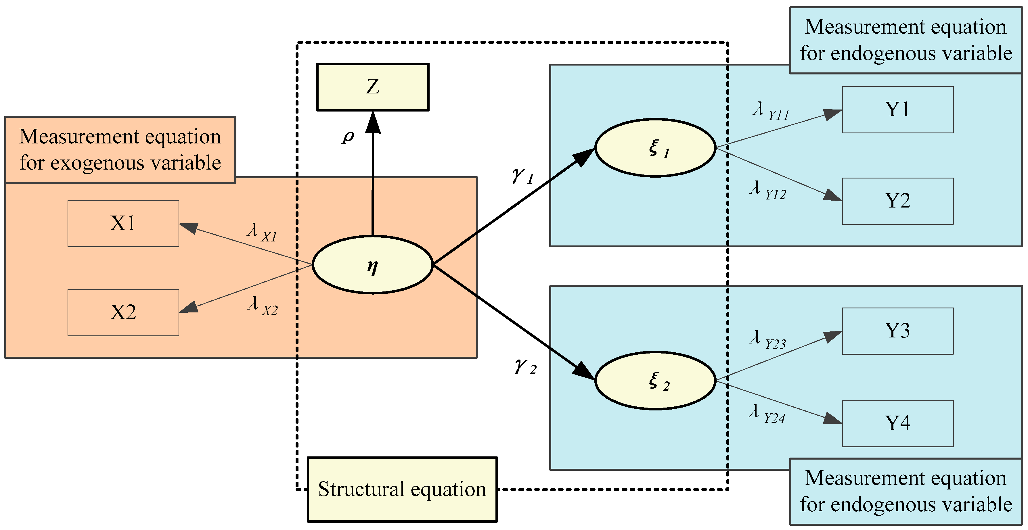
Figure 1 shows a simple schematic diagram of SEM along with the various kinds of variables. The equations of SEM are specified by direct links between these variables, which can be called “the simultaneous equations” [30]. SEM is defined using three sets of equations: structural equations, and measurement equations for both the endogenous and exogenous variables [31]. The purpose of the structural equations is to capture causation and weight the influence of exogenous variables (η) on endogenous variables (ξ1 and ξ2), and relationships between latent variables and those observed variables (Z) without latent variables. The measurement equations are composed of latent variables (η, ξ1 and ξ2) and their observed variables (X1, X2; Y1, Y2, Y3, and Y4), which are used to capture the relationship between the two kinds of variables. λ represents coefficient matrix between latent variables and their observed variables. γ represents matrix of regression effects for exogenous variables to endogenous variables.
Before applying SEM, hypotheses regarding causal relationships between variables need to be proposed [32]. Then, SEM can obtain more valid coefficients and provide more support for testing and confirming these hypotheses [33,34,35]. In the process of SEM development, a two-step approach is the most widely used method present [36]. The first step is to develop an acceptable measurement model through confirmatory factor analysis (CFA). The measurement model describes how well the latent variables are measured by their observed variables. However, causal relationships between the latent variables are not specified by the measurement model [37]. Therefore, in the second step, the structural model is modified to describe the relationships among the latent variables. The modified model is usually referred to as the structural model or the causal model [28].
Measurement model fit should be evaluated by assessing convergent validity and discriminant validity. Convergent validity and discriminant validity attempt to test whether observed variables correspond to the latent variables [38]. Convergent validity means that observed variables, which should theoretically be related to each other, are practically observed to be related to each other. Discriminant validity means latent variables, which should theoretically not be related to each other, are practically observed to not be related to each other. In this paper, the method of factor loading was applied to assess convergent validity. Composite reliability (CR) is one of the most important indexes to test the convergent validity, which can be evaluated by Equation (1) [39]. In the equations, λ donates the factor loading and θ means the variance of measurement errors. Generally, the value of CR theoretically should be more than 0.6. The method of chi-square difference quantity was used to test discriminant validity. To evaluate the difference value of chi-square, two measurement models were established including unrestricted model and restricted model. The difference between the two models was that the co-variation parameter between latent variables of unrestricted model was freely estimated parameter, while that of restricted model was fixed parameter. If the difference value of chi-square is high and reaches the significance level, it means that the two measurement models are discriminated from each other. Moreover, the lower the chi-square value of unrestricted model is, the higher the value of discriminant validity will be.
Criteria were developed based on the chi-square statistics given by the result of the optimized fitting function and the sample size. These criteria can also measure how well one model functions compared to another model. Firstly, the sample size cannot be too small and a critical sample size of N = 200 was set for an acceptable model [40]. Common goodness-of-fit measures for a single model are as follows [41]: (1) root mean square error of approximation (RMSEA), which measures the discrepancy per degree of freedom; (2) the comparative fit index (CFI); (3) the goodness-of-fit index (GFI); (4) the adjusted goodness-of-fit index (AGFI); and (5) the normed fit index (NFI). Most SEM programs provide these measures together with their confidence intervals. As a general rule, the value of RMSEA for a good model should be less than 0.05 while the CFI, AGIF, CFI, NFI should be more than 0.90 [42].
Compared with other traditional multivariate statistical methods, SEM has several advantages: Firstly, it can estimate the effect of observed variables on both exogenously and endogenously latent variables simultaneously, which cannot be measured through a survey. Secondly, in SEM, variables can be either exogenous or endogenous, which allow the method to handle indirect, multiple, and reverse relationships [34,35]. In other words, the causal relationships between the independent variables can also be estimated, which is difficult to achieve using other methods. Finally, the graphical and intuitive expression of the results makes it much easier for us to visualize the complicated relationships between large numbers of variables [38,43].
Most existing studies on long-distance travel behavior are limited to directive analyses of the relationship between mode choice and influential factors, while the internal mechanism has rarely been discussed. According to the above stated, SEM has advantages over handling complicated relationships between numerous variables. Therefore, SEM is used in this paper to explore the intricate relationships between the various factors and the complicated travel mode choice behavior characteristics.
3. Methods
3.1. Survey
To obtain the basic information about passengers’ travel mode choice behavior in China, a survey was conducted in Beijing at four different transportation stations, namely Beijing Railway Station (the largest ordinary railway station in Beijing), Beijing South Railway Station (the largest HSR station), Beijing Capital Airport, and Beijing Liuliqiao long-distance bus station. At each survey site, 100 effective questionnaires were collected during November and December 2012.
Passengers’ travel mode choices among coach, ordinary train, HSR and plane is the dependent variable in this survey, and the explanatory variables mainly include passengers’ socio-demographic characteristics (such as gender, age, education level, vocation and income), service preference characteristics, i.e., passengers’ preference for a travel mode’s different service elements (such as preference for safety, economy, comfort, and punctuality), performance satisfaction characteristics, i.e., passengers’ satisfaction on a travel mode in each aspect of service elements (such as safety, economy, efficiency, comfort and punctuality), and trip characteristics (such as departure time and travel distance).
3.2. Data and Independent Variables
Of 400 cases collected, 33 cases were excluded because of missing values or unreasonable data. As a result, the number of valid responses in this study was 367 with a 91.75% retention rate. Table 1 is relevant statistical information about passengers’ socio-demographic characteristics. Passengers’ education level is divided into three different levels, including low-education, middle-education and high-education. The low level includes passengers who have never been to a university. The middle level includes passengers who are studying for or have obtained a bachelor’s degree. The high level includes passengers whose are studying for or have obtained a graduate degree. Passengers’ income level is divided into three categories. The first category is low-income passengers, whose income is less than 6 thousand RMBRMB (¥) per month. The second category is middle-income passengers, whose income is between 6 thousand and 10 thousand RMB per month. The last category is high-income passengers, whose income is more than 10 thousand RMB per month.
Table 2 lists the statistical information about passengers’ service preference distribution. For each service element, passengers’ preference is divided into five levels, from the most important to the least important. Particularly, when passengers treat a service element as the most important, it means that they care most about whether travel modes perform well. It could be found that safety and price are the most two important service elements. Of the 367 respondents, 285 passengers cared most about whether modes for the long-distance travel were safe, while 128 considered price as the second important aspect of travel modes.
To intuitively demonstrate passengers’ service element preference for long-distance travel, the average importance score of each service element was calculated by defining value of each importance level, ranging from five points for the most important level to one point for the least important level, as listed in Table 2. According to Figure 2, the safety (4.58 points) was the most important service element, followed by price (2.88 points), comfort (2.62 points), punctuality (2.50 points) and efficiency (2.42 points).
Figure 3 shows the satisfaction distribution of each travel mode in terms of different service elements, reflecting which travel modes were the most or least competitive in specific aspects. The ordinary train had the most advantages on both safety and economy among the four modes; however, it was least competitive in terms of efficiency, comfort and punctuality. HSR was most competitive in aspects of efficiency, comfort and punctuality. Plane ranked highly for efficiency and comfort but was less competitive than HRS for both. The coach was the least competitive mode for long distance travel in every aspect, and could therefore be termed the least competitive overall.
Respondents were also asked to make travel mode choice under different assumptive departure time and travel distance ranges, to explore the influence of trip attributes on mode choice. Thus, the departure time and travel distance in this study can be regarded as two repeated variables, which means that a respondent must choose one travel mode at different departure time and distance ranges, while the other three kinds of explanatory variables remain the same. In this study, it is simplified that the passengers depart either at daytime or at night. The travel distance is divided into five intervals, <500 km, 500–1000 km, 1000–1500 km, 1500–2000 km and >2000 km. Therefore, each respondent has to make ten repeated mode choice decisions.
4. Descriptive Analyses
The analysis of variance (ANOVA) approach was applied to investigate the impacts of independent variables on passengers’ travel mode choice behavior, and the hypothesis testing of the coefficients was based on a 0.05 significance level. Table 3 reports the ANOVA results for the differences between factors. It could be found that, except gender (F = 0.5, p > 0.05), service preference for safety (F = 3.2, p > 0.05) and departure time (F = 2.3, p > 0.05), all other variables significantly influenced the passengers’ travel mode choice behavior.
4.1. Effects of Passengers’ Socio-Demographic Characteristics on Mode Choice
Table 4 displays the statistical information of passengers’ travel mode choice behavior based on different categories of independent variables about passengers’ socio-demographic characteristics. In Table 4, the following general passengers’ travel mode choice behavior characteristics can be identified.
First, HSR is the most competitive travel mode among all age groups, the selection proportions of which are all above 30%. Inversely, coach has no competitiveness among all age groups. Except for HSR, ordinary train is relatively more popular with those below 30 years old or above 50 years old, while plane is more competitive among passengers in the age group of 30 to 50 years old.
Second, there are some differences in travel mode choice of passengers with different education levels. As expected, passengers with higher education level are obviously more likely to choose plane. Particularly, 43.2% of passengers with high education level choose plane to travel, much higher than 29% and 21.8% of those with middle and low education level, respectively. Conversely, the percentages of passengers with high education level ordinary train are much lower than those of s passengers with middle and low education level, 14% versus 29.2% and 30.5%, respectively.
Third, passengers’ vocation has a big impact on their travel mode choice. Figure 4 illustrates relationship between vocation and travel mode choice. According to the mode choice distribution patterns, the passengers’ vocations can be categorized three clusters. In Cluster #1, the choices of student, farmer and worker were very similar while most of them preferred to choose ordinary train and HSR rather than coach and plane. In Cluster #2, free vocation passengers’ mode choice pattern is close to small business owners, who are most likely to choose HSR. In Cluster #3, civil servants and enterprise employees, who have the highest income level, are most likely to choose plane with the highest travel expense.
Finally, significant differences can be observed between travel mode choices among passengers with different income levels. It could be found that coach was not competitive among three groups of passengers while HSR was always passengers’ favorite travel mode. Specifically, the average selected portions of coach and HSR of the three groups of passengers are 10.6% and 33.2%, respectively. However, the results showed that passengers’ choices of coach and HSR did not show great changes in different income levels. The lowest and highest selected portions of coach among the three groups are 9.2% and 11.4%, and that of HSR are 32% and 34.3%. Inversely, income level was much more sensitive to ordinary train and plane. Passengers with higher income level would more likely to choose plane while ordinary train may be chosen by passengers with relatively low income. Particularly, the lowest and highest selected portions of ordinary train among the three groups are 13.2% and 33.3%, and that of plane are 21% and 44.2%. The trend was quite similar to the relationship between education level and travel mode choice. The reason might be that people’s income level is highly correlated with education level [44,45].
4.2. Effect of Service Preference Attributes on Mode Choice
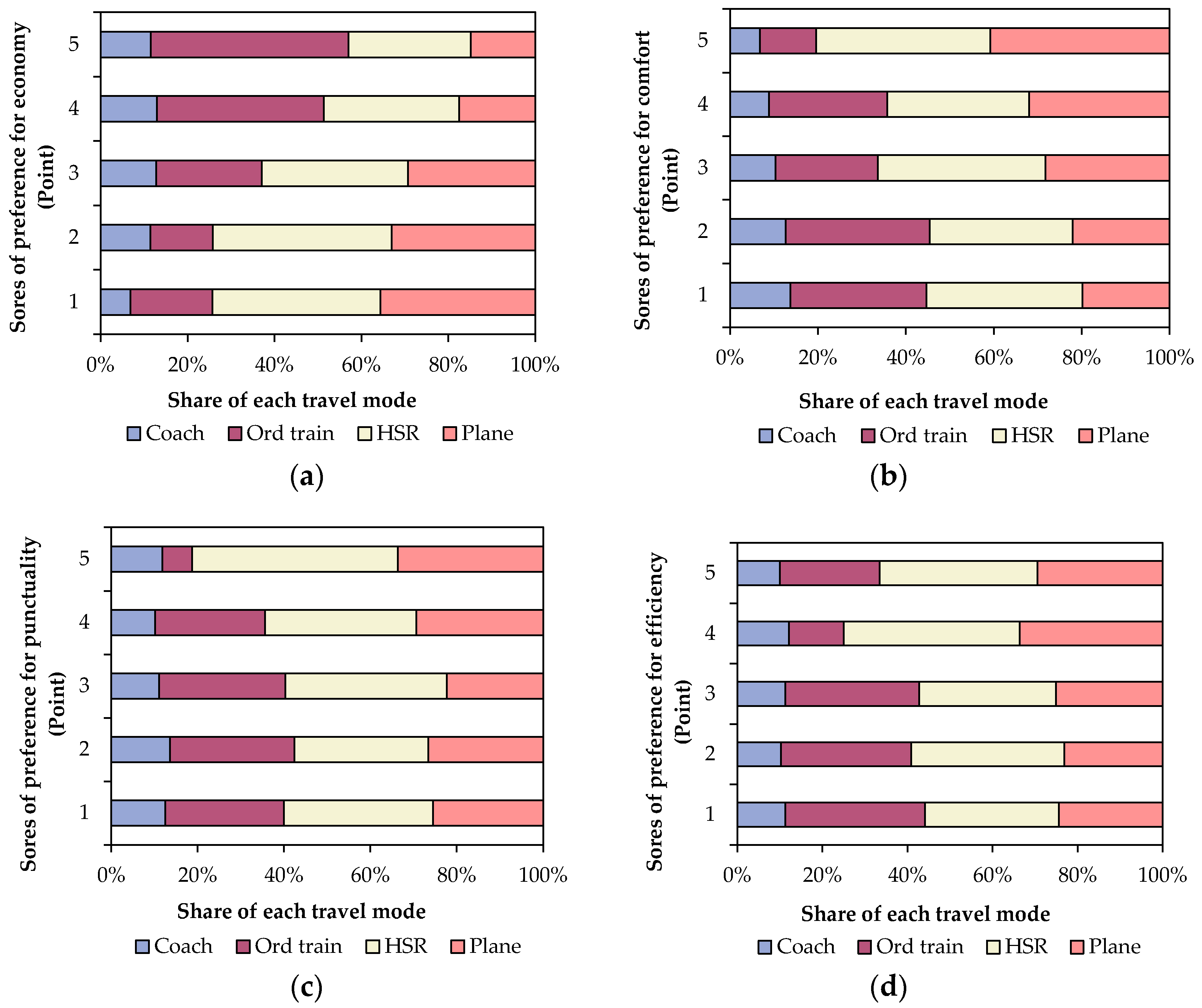
Figure 5 illustrates the relationship between travel mode choice and different importance levels of service preference for economy, comfort, punctuality and efficiency respectively. The results showed that different preferences would result in passengers’ different mode choice behavior. Figure 5a indicates that, in the long-distance travel, ordinary train may be chosen more over the three other travel modes for those caring more about the travel expense, whereas plane and HSR may be chosen more over coach and ordinary train when passengers cared less about money. One possible reason for this phenomenon was that the prices of HSR and plane were much higher because the target customer of the HSR and plane was mid- and top-earners [16,46]. In contrast, Figure 5b reveals that passengers were more likely to choose HSR and plane when they paid more attention to whether the travel mode was comfortable. Similar choice tendency about preference of punctuality and efficiency could be found from Figure 5c,d, respectively. The results also implied that HSR and plane would be considered as the modes that could shorten travel time and provide a high quality of service. Such a finding was consistent with the previous study [47]. Therefore, to enhance the competitiveness of travel modes, the transport operator should target the passengers’ service preference and provide diversified services to different target passenger groups.
4.3. Effect of Performance Satisfaction Attributes on Mode Choice
Generally, when a passenger thought that a travel mode was the most competitive in one service element, it meant that the passenger was satisfied with the travel mode’s service performance. In this study, the satisfaction score on a travel mode’s service performance was calculated as 0 or 1 point: if a travel mode was considered as was the most competitive in one service element, the satisfaction score for the mode would be 1 point; otherwise, the score would be zero. Figure 6a illustrates each travel mode’s average satisfaction score on the overall performance in the aspects of safety, economy, efficiency, comfort and punctuality. Figure 6b illustrates the distribution of passengers’ travel mode choices, indicating a similar distribution pattern of the average satisfaction scores in Figure 6a. It could be found that HSR was the passengers’ most satisfied travel mode with absolute advantage (2.29 points), corresponding to the highest mode choice percentage (34%). The finding implied that the more passengers were satisfied with the service of travel modes, the more likely they would be to choose them. Thus, to seize the shares of passenger transportation market, transport operators are required to improve their service performance and get passengers’ high recognition.
4.4. Effect of Travel Distance on Mode Choice
The results revealed that travel distance significantly affected passengers’ long-distance travel mode choices. Generally, when the travel distance was relatively long, passengers would be more inclined to choose plane and HSR, whereas ordinary train or coach would be chosen over plane and HSR within relatively short distance. Figure 7 illustrates the different levels of competitiveness of the travel modes over different distance. It showed that the competitiveness of plane and coach contrasted with each other. When the travel distances increased, plane would be much more competitive while coach was much less so. However, the trends in ordinary trains and HSR were very similar to each other and did not show monotonous changes in competitiveness over different distances. The competitiveness of both ordinary trains and HSR increased at first and then decreased.
To further understand the competition between travel modes over different distances, the competitiveness over each distance range was analyzed. When the travel distance was less than 500 km, the coach (38.91%) was the most competitive travel mode followed by the ordinary train (33.06%) and then HSR (26.67%); the plane mode was almost completely uncompetitive with only 1.36% of passengers choosing them. It meant that passengers would tend to choose coach and ordinary train over HSR and plane within the distance of 500 km. Similarly, Zhang and Zhao [48] found that, when the distance was less than 300 km, the main competition was between the railway and coach. Furthermore, the share of ordinary trains was higher than that of HSR. One possible explanation was that the speed advantage of HSR was unapparent when the distance was short, so that passengers were more likely to choose ordinary trains due to their low prices. Within the distance range from 500 km to 1000 km, the competitiveness of ordinary train, HSR and plane was all increasing while the coach mode’s competitiveness was dramatically decreasing; it should be note that the share of the ordinary train achieved its highest point (40%) within the distance interval. The results revealed that passengers would be likely to choose ordinary train and HSR over coach and plane within the distance from 500 km to 1000 km. Within the distance range from 1000 km to 1500 km, the share of passengers choosing the ordinary railway began to fall, while HSR experienced no change (remaining at 42%), which meant that HSR was often considered as the best transportation mode for medium-distance trips [47]. When the travel distance was between 1500 and 2000 km, the share of plane started to be similar to HSR and even became the most competitive travel mode. When the travel distance was over 2000 km, the plane was the most competitive travel mode, with an absolute advantage (60.57%), followed by HSR (24%), ordinary train (14%) and coach (2%). In summary, considering the highest share as the measurement of competitiveness, the most competitive range of coach was below 500 km; for ordinary train it was about 500–1000 km; for HSR it was 500–1500 km; and for plane it was over 1500 km.
4.5. Summarization on Travel Modes’ Competitiveness and Relevant Suggestions
Based on the above analyses, Table 5 summarizes each travel mode’s competitive travel distance scope, performance features about service elements and target passenger groups. In addition, relevant suggestions were proposed to increase each travel mode’s competitiveness and serviceability.
Except for spatial competitiveness within the travel distance of 500 km, coach was uncompetitive over all aspects of service performance among almost every passenger group. Transport operators of coach were facing great challenges in how to boost the passenger transportation market share. The results revealed that the service quality improvement may assist in attracting more passengers. Planners should promote the accessibility of bus stations and networks between adjacent cities to provide proper environments for short haul.
Because of the low travel expense, ordinary train was popular among passengers with relatively lower-income, such as students, famers and works. However, due to the low service quality on the aspects of efficiency, comfort and punctuality, ordinary train was not attractive to passengers with high-income, since their travel demand has transformed from a unitary pattern of accessibility to a pluralist coexistent pattern of accessibility and enjoyment. In this case, the efforts to investigate passengers’ service preference could be made in providing reasonably diversified services to different target passenger groups. Transport planners should take full advantage of its superiority within the competitive distance scope, 500–1000 km. In the future, enhancing infrastructure construction of ordinary train in the middle-long distance may make it more attractive.
HSR was competitive within almost all travel distance scope and the most satisfied travel mode among each passenger group. The results may bring massive encouragements for the government to further develop the HSR networks. As of 2014, the construction of four vertical and four horizontal trunk lines, proposed in the “Medium and Long Term Railway Network Planning” of China, has made a significant progress with all four vertical trunk lines under operation. In the future, the government should simultaneously accelerate the construction of branch lines to improve the capacity of HSR network and meet the dramatically increasing demand of passengers. Moreover, the fact that travel expense of HSR was slightly high [46] suggests that passengers would be enticed by economic incentives, such as ticket discount and bonus points, especially for those with low-income travelers.
The performance of punctuality was one of the main restricts in competitiveness of plane. Thus, operators should strive to ensure the travel time reliability. Plane was considered as a luxury travel mode with high income-elastic [7], which should attract the passengers with high-income, such as civil servant and enterprise employee, as target passenger groups. Though a high discount rate may flexibly occur in the air transportation, a sizeable portion of passengers was obviously transferred from air mode to the HSR mode owing to lower price but more reliable travel time, especially within the travel scope ranging from 500 km to 2000 km. Thus, operators should further devote to taking proper economic incentive strategies, for example reducing the airport construction fee and fuel oil tax. On the other hand, plane should consolidate the passenger transportation market share in its advantage distance scope, i.e., over 2000 km.
Toward the end, great efforts are required to construct a reasonable comprehensive transportation network and improve the multi-mode passenger transportation market in the long-distance travel. Infrastructure construction of each mode should be strengthened within its competitive distance range in order to fully take advantage of each travel mode’s superiority. At the same time, transport managers should develop the market segmentation strategy to lead the market differentiation, and operators should provide diversified and high-quality service to improve passengers’ satisfaction.
5. SEM Development and Results
5.1. Variables System and Models
As listed in Table 6, in this study, the structural equation includes three latent variables, and two observed variables without latent variables. Particularly, personal attributes are specified as a latent variable while education level, vocation and income level were considered to be its observed variables. Service preference attributes and performance satisfaction attributes are the other two latent variables, which, respectively, have four and five observed variables. Moreover, the passengers’ travel mode choice is the endogenous variable. Table 6 shows the relationship between latent variables and their observed variables, as well as the descriptions and input codes for the observed variables adopted in the following analysis.
In this paper, two hypotheses are proposed for explaining the passengers’ travel mode choice behavior. Firstly, it is assumed that above three latent variables, as well as the observed variable of travel distance have a significant impact on the passengers’ choice of travel mode. Secondly, it is assumed that the latent variable of personal attributes significantly affects latent variables of service preference attributes and performance satisfaction attributes. To test whether these variables have an impact on mode choice, four arrows from three latent variables (personal attributes, service preference attributes and performance satisfaction attributes) and the observed variable (travel distance) to the observed variable (travel mode choice) were connected. Furthermore, two linkages between the latent variable (personal attributes) and latent variables (service preference attributes and performance satisfaction attributes) were examined. Therefore, as shown in Figure 8, a testing structural model was developed to verify the two hypotheses of passengers’ travel mode choice behavior in long-distance.
5.2. Verification of Hypotheses: Structural Model of Passengers’ Travel Mode Choice
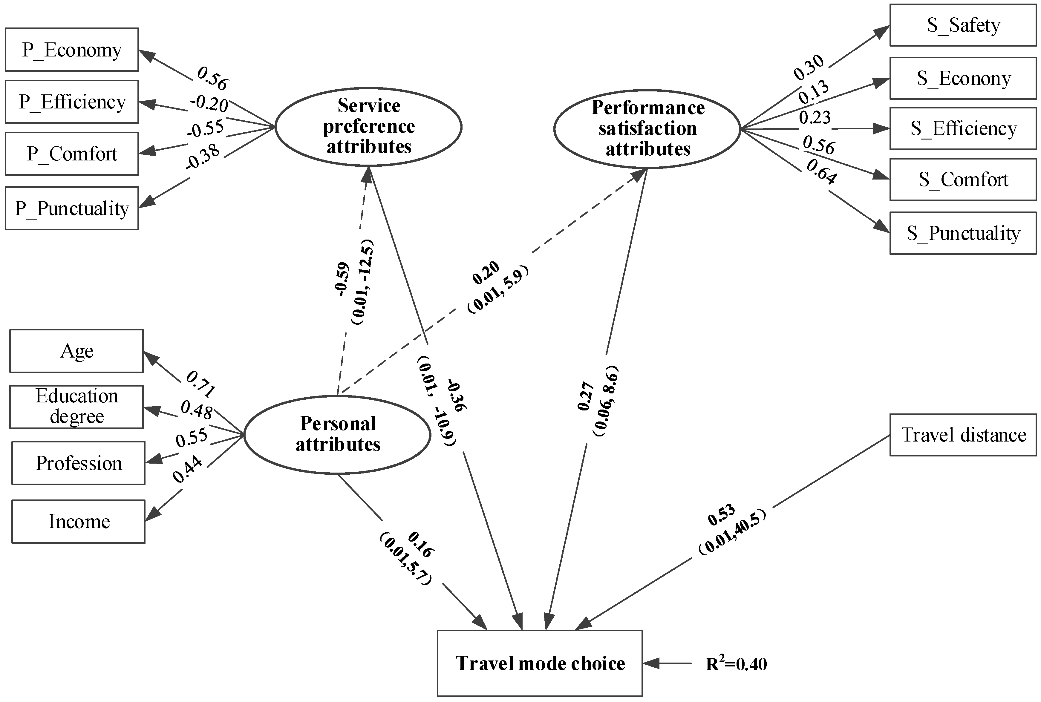
Modified by the rules of assessing goodness-of-fit [28], an acceptable travel mode choice model with high fitted values was achieved, as shown in Figure 8. Standardized loading factors along with the standard error of the estimate and the critical ratio were shown in the figure. The numbers on the arrows were parameter estimates and the numbers in parentheses indicated the standard errors and critical ratio, the latter being equivalent to the t-value. If the t-value was greater than 1.96, then the estimate was significant at the 95% confidence level.
Table 7 lists the results of the hypothesis verification. From the parameters of measurement models and the travel mode choice structural model, the results of the hypothesis verification could be described as follows:
Firstly, all the observed variables in the final model were significant in measuring their latent variables. After estimating by software AMOS, it could be found that the CR of measurement model for exogenously latent variable (personal attributes) was 0.6, and that of measurement model for exogenously latent variable (service preference and performance satisfaction) was 0.8. The results showed that the observed variables of each latent variable were related to each other and convergent validity was high. The chi-square value of unrestricted model was 234.4 and that of restricted model was 2684.4. The difference value of chi-square was 2450, and the probability value of chi-square difference quantity significance test was p = 0.000, reaching the significant level (p < 0.05). The results meant that there was significantly difference between the unrestricted model and restricted model, i.e., the three latent variables were discriminated from each other. Compared with restricted model, the chi-square of unrestricted model was smaller, meaning that discriminant validity between the three latent variables was high.
Secondly, three latent variables including personal attributes (t = 5.7, p < 0.05), service preference attributes (t = −10.9, p < 0.05), and performance satisfaction attributes (t = 10.7, p < 0.05)), as well as the observed variable travel distance (t = 40.5, p < 0.05) all had a significant impact on the passengers’ travel mode choice. Moreover, the results suggested that travel distance (factor loading = 0.53) was the most significant factor, followed by service preference attributes (factor loading = −0.36), performance satisfaction attributes (factor loading = 0.27) and personal attributes (factor loading = 0.16). Specifically, among the four observed variables of service preference attributes, the preference for economy was the most important factor influencing mode choice, with an impact factor of 0.20 (0.56 × 0.36), followed by the preference for comfort with 0.19 (0.55 × 0.36), punctuality with 0.14 (0.38 × 0.36) and efficiency with 0.07 (0.20 × 0.36). Furthermore, among the five observed variables of performance satisfaction attributes, satisfaction on comfort was the most significant factor influencing mode choice, with an impact factor of 0.18 (0.64 × 0.27), followed by satisfaction on efficiency with 0.15 (0.56 × 0.27), punctuality with 0.08 (0.30 × 0.27), economy with 0.06 (0.23 × 0.27) and safety with 0.04 (0.13 × 0.27).
Finally, the latent variable of personal attributes had a significant impact on the latent variables of service preference attributes (factor loading = −0.59, t = −12.5, p < 0.05) and performance satisfaction attributes (factor loading = 0.20, t = 5.9, p < 0.05). The results revealed that except for the above direct impact, the personal attributes also had an indirect influence on the mode choice in the way of affecting service preference attributes and performance satisfaction attributes. Table 8 lists both the direct and indirect effects of latent variable (personal attributes) and its observed variables (age, education level, vocation and income) on the travel mode choice behavior. The results showed that the indirect effect (0.27) of personal attributes was higher than direct effect (0.16), which meant that the two mediating variables (service preference attributes and performance satisfaction attributes) played a necessary role in the influence of personal attributes on the travel mode choice [43,49].
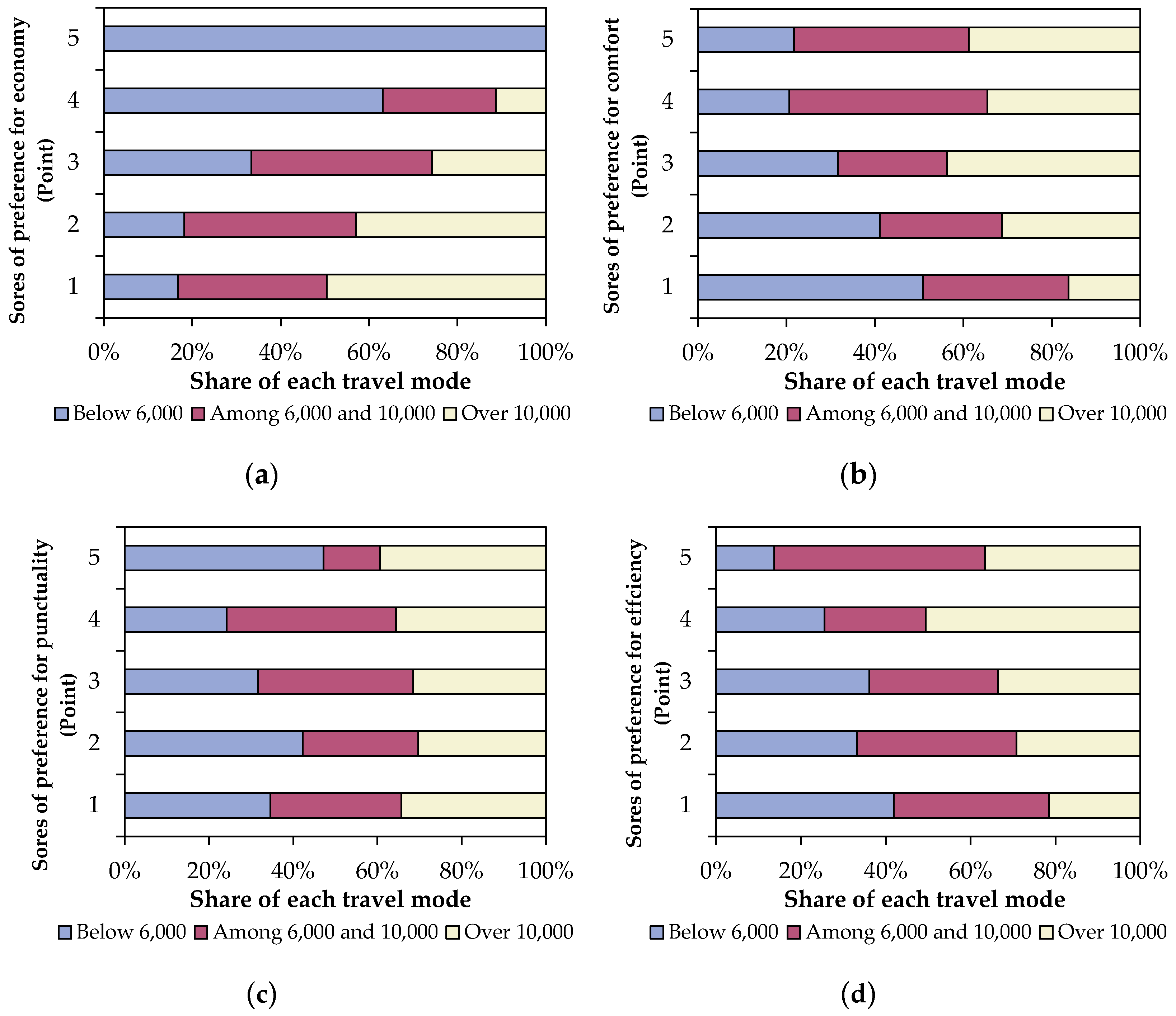
Particularly, as shown in Figure 9, the results reveal that passengers with different income level showed great difference in service element preference of travel modes, especially in economy and comfort. Passengers with high income would be more concerned about the travel mode’s comfort, efficiency and punctuality but less about travel expense, while passengers with lower income immensely cared about whether the mode could save money. A similar result was shown by Ye and Wang [50], who found that with an increase of income, the sensitivity of the travel expense dropped while the sensitivity to journey time increased. Analogously, such results could be found in Vocation Cluster #2 (free vocation and small business owner), Vocation Cluster #3 (civil servant and enterprise employee), and passengers with higher education level or age. Moreover, the results show that passengers with higher income, education level and age may be more satisfied with HSR and plane. In addition, the satisfaction degree on the performance of HSR and plane was higher among Vocation Cluster #2 (free vocation and small business owner) and Vocation Cluster #3 (civil servant and enterprise employee) but lower among Vocation Cluster #1 (students and peasants).
5.3. Fit Indices of SEM Model
Table 9 summarizes the goodness-of-fit statistics of the three SEM models explored in this paper. According to the results, except for the p-value of the structural model (p-value < 0.05), almost all the values of GFI, AGFI, CFI, and NFI are greater than 0.9 and the values of RMSEA are smaller than 0.05, which indicates that the model matches the data well and is acceptable. Generally, the p-value should be more than 0.05 but when the sample size is large, the p-value will be deeply affected and will incline towards zero. Thus, even if the p-value of the structural model is smaller than 0.05, the result can still be acceptable [49]. The structural model explained 40% (R2 = 0.40) of the total variance in passengers’ travel mode choice.
6. Conclusions
China has entered a period of rapid development of high-speed rail (HSR), which brings an intense competition to the other long-distance travel modes. Travel mode choice is a complex psychological and behavioral process influenced by various factors. In this study, the potential influencing factors as well as their causal relationship were explored to understand passengers’ long-distance travel mode choice behavior characteristics.
Potential influencing factors are verified whether have significant impact on passengers’ travel mode choice behavior based on the analysis of variance (ANOVA) approach. The results reveal that, except gender, service preference safety and departure time, all other variables significantly influence the passengers’ travel mode choice behavior. Specifically, for personal attributes, some important findings have been obtained: firstly, passengers with higher education level are obviously more likely to choose plane; secondly, according to the mode choice distribution patterns, the passengers’ vocations can be categorized into three clusters; and, finally, income level was sensitive to ordinary train and plane, while passengers with higher income level would more likely to choose plane and ordinary train may be chosen by passengers with relatively low income. For service preference attributes, it is found that ordinary train may be chosen more for those caring more about travel expense, whereas plane and HSR may be chosen more when passengers paid more attention to whether the travel mode was comfortable, punctuality and efficiency. For performance satisfaction attributes, the results show that the more passengers were satisfied with the service of travel modes, the more likely they would be to choose them. For travel distance attribute, it can be concluded that the most competitive distance ranges for coach, ordinary train, HSR and plane were below 500 km, 500–1000 km, 500–1500 km and over 1500 km, respectively.
SEM method is used to test the causal relationship between the influencing factors. The results reveal that travel distance was the most significant variable affecting travel mode choice followed by service preference attributes, performance satisfaction attributes and personal attributes. Furthermore, except for the direct impact, personal attributes are verified to have an indirect influence on passengers’ travel mode choice behavior by significantly affecting service preference and performance satisfaction attributes. Particularly, passengers with older ages and higher incomes and education levels would concern more about whether the travel mode was comfortable, efficient and punctual and cared less about economy. In addition, they were more satisfied with HSR and plane. Free vocation, small business owner, civil servant and enterprise employee tended to have similar patterns in the service preference (more comfort, efficiency and punctuality and less economy) and performance satisfaction (more satisfied with HSR and plane) while the patterns in student, farmer and worker were opposite to the other vocations.
In summary, the long-distance travel mode choice behavior profoundly affects the establishment of the public transportation service market. Through research into the long-distance travel mode choice, the public transportation users’ preferences to different travel modes can be identified, and transportation management and resource allocation can be implemented more effectively by policy makers.
Acknowledgments
This work is financially supported by the National Natural Science Foundation of China (71621001), and the Fundamental Research Funds for the Central Universities (2016YJS080).
Author Contributions
Y.W. and X.Y. conceived and designed the survey; Y.W., Y.Z., and Q.X. conducted the survey; Y.W., Y.Z., and Q.X. process the data; and Y.W., X.Y. and Y.Z. analyzed the data, interpreted the findings and wrote the paper. All authors have read and approved the final manuscript.
Conflicts of Interest
The authors declare no conflict of interest.
References
- National Bureau of Statistics of China. Available online: http://www.stats.gov.cn/ (accessed on 19 October 2017).
- Liu, J.; Zhang, N. Empirical Research of Intercity High-speed Rail Passengers’ Travel Behavior Based on Fuzzy Clustering Model. J. Transp. Syst. Eng. Inf. Technol. 2012, 12, 100–105. [Google Scholar] [CrossRef]
- Fu, X.; Zhang, A.; Lei, Z. Will China’s airline industry survive the entry of high-speed rail? Res. Transp. Econ. 2012, 35, 13–25. [Google Scholar] [CrossRef]
- Nostrand, C.V.; Sivaraman, V.; Pinjari, A.R. Analysis of long-distance vacation travel demand in the United States: A multiple discrete–continuous choice framework. Transportation 2013, 40, 151–171. [Google Scholar] [CrossRef]
- Lu, Y.J.; Zhang, L. Imputing Trip Purposes for Long-Distance Travel. Transportation 2015, 42, 581–595. [Google Scholar] [CrossRef]
- Reichert, A.; Rau, C.H. Mode use in long-distance travel. J. Transp. Land Use 2015, 8, 87–105. [Google Scholar] [CrossRef]
- Dargay, J.M.; Clark, S. The determinants of long distance travel in Great Britain. Transp. Res. Part A 2012, 46, 576–587. [Google Scholar] [CrossRef]
- Arbués, P.; Baños, J.F.; Mayor, M.; Suárez, P. Determinants of ground transport modal choice in long-distance trips in Spain. Transp. Res. Part A 2016, 84, 131–143. [Google Scholar] [CrossRef]
- Sung, H.G. Determinants of Transportation Mode Choice for Long-distance Travel in Korea - Focused on High-speed Rail over Private Car. J. Korea Plan. Assoc. 2014, 49, 245–257. [Google Scholar] [CrossRef]
- Lu, Q.C.; Zhang, J.; Peng, Z.R.; Rahman, A.B.M.S. Inter-City Travel Behaviour Adaptation to Extreme Weather Events. J. Transp. Geogr. 2014, 41, 148–153. [Google Scholar] [CrossRef]
- Kim, S.; Ulfarsson, G.F. Travel mode choice of the elderly: Effects of personal, household, neighborhood, and trip characteristics. Natl. Res. Counc. 2004. [Google Scholar] [CrossRef]
- Georggi, N.L.; Pendyala, R.M. Analysis of Long-Distance Travel Behavior of the Elderly and Low Income. Transp. Res. Circ. 2012, E-C026, 121–150. [Google Scholar]
- Mallett, W.J. Long-distance travel by low-Income households. TRB Transp. Res. Circ. 2001, E-C026, 169–177. [Google Scholar]
- Santos, G.; Maoh, H.; Potoglou, D.; von Brunn, T. Factors influencing modal split of commuting journeys in medium-size European cities. J. Transp. Geogr. 2013, 30, 127–137. [Google Scholar] [CrossRef]
- Mabit, S.L.; Rich, J.; Burge, P.; Potoglou, D. Valuation of travel time for international long-distance travel results from the Fehmarn Belt stated choice experiment. J. Transp. Geogr. 2013, 33, 153–161. [Google Scholar] [CrossRef]
- Wang, S.; Zhao, P. Analysis of passengers’ choice behavior for dedicated passenger railway lines based on Logit model. J. China Railw. Soc. 2009, 31, 6–10. [Google Scholar]
- Abdel-Aty, M.; Jovanis, P. A Survey of the Elderly: An Assessment of Their Travel Characteristics. In Proceedings of the 77th Annual Meeting of the Transportation Research Board, Washington, DC, USA, 11–15 January 1998. [Google Scholar]
- Redman, L.; Friman, M.; Gärling, T.; Hartig, T. Quality attributes of public transport that attract car users: A research review. Transp. Policy 2013, 25, 119–127. [Google Scholar] [CrossRef]
- Yu, C.C. Factors affecting airport access mode choice for elderly air passengers. Transp. Res. Part E 2013, 57, 105–112. [Google Scholar]
- Paulley, N.; Balcombe, R.; Mackett, R.; Titheridge, H.; Preston, J.; Wardman, M.; Shires, J.; White, P. The demand for public transport: The effects of fares, quality of service, income and car ownership. Transp. Policy 2006, 13, 295–306. [Google Scholar] [CrossRef]
- Janic, M. A model of competition between high speed rail and air transport. Transp. Plan. Technol. 1993, 17, 1–23. [Google Scholar]
- Rothengatter, W. Competition between airlines and high-speed rail. In Critical Issues in Air Transport Economics and Business; Macario, R., van de Voorde, E., Eds.; Routeledge: Oxford, UK, 2011. [Google Scholar]
- Gonzalez-Savignat, M. Competition in air transport: The case of the high speed train. J. Transp. Econ. Policy 2004, 38, 77–108. [Google Scholar]
- Parkan, C. Measuring the operational performance of a public transit company. Int. J. Oper. Prod. Manag. 2002, 22, 693–720. [Google Scholar] [CrossRef]
- Su, F.; Bell, M.G.H. Transport for older people: Characteristics and solutions. Transp. Econ. 2009, 25, 46–55. [Google Scholar] [CrossRef]
- Yin, H.; Guan, H.; Liu, T.; Gong, L. Study of urban resident travel mode choice behavior. In Proceedings of the 10th International Conference of Chinese Transportation Professionals—Integrated Transportation Systems: Green, Intelligent, Reliable, ICCTP 2010, Beijing, China, 4–8 August 2010. [Google Scholar]
- Wu, J.; Yang, M. Modeling Commuters’ Travel Behavior by Bayesian Networks. Procedia Soc. Behav. Sci. 2013, 96, 512–521. [Google Scholar] [CrossRef]
- Golob, T.F. Structural equation modeling for travel behavior research. Transp. Res. Part B 2003, 37, 1–25. [Google Scholar] [CrossRef]
- Roorda, M.J.; Ruiz, T. Long- and short-term dynamics in activity scheduling: A structural equations approach. Transp. Res. Part A 2008, 42, 545–562. [Google Scholar] [CrossRef]
- Lee, J.; Chung, J.; Son, B. Analysis of traffic accident for Korean highway using structural equation models. Accid. Anal. Prev. 2008, 40, 1955–1963. [Google Scholar] [CrossRef] [PubMed]
- Sharmeen, F.; Arentze, T.; Timmermans, H. An analysis of the dynamics of activity and travel needs in response to social network evolution and life-cycle events: A structural equation model. Transp. Res. Part A 2014, 59, 159–171. [Google Scholar] [CrossRef]
- Chen, Y.; Lin, L. Structural equation-based latent growth curve modeling of watershed attribute-regulated stream sensitivity to reduced acidic deposition. Ecol. Model. 2010, 221, 2086–2094. [Google Scholar] [CrossRef]
- Dion, P. Interpreting structural equation modeling. Bus. Ethics 2008, 83, 365–368. [Google Scholar] [CrossRef]
- Iriondo, J.M.; Albert, M.J.; Escudero, A. Structural equation modeling: An alternative for assessing causal relationships in threatened plant populations. Biol. Conserv. 2003, 113, 367–377. [Google Scholar] [CrossRef]
- Martinez, L.; Silva, J.; Viegas, J. Assessment of residential location satisfaction in the Lisbon metropolitan area. Available online: https://trid.trb.org/view.aspx?id=909819 (accessed on 19 October 2017).
- Anderson, J.C.; Gerbing, D.W. Structural equation modeling in practice: A review and recommendation two-step approach. Psychol. Bull. 1988, 103, 411–423. [Google Scholar] [CrossRef]
- Hassan, H.M.; Abdel-Aty, M.A. Analysis of drivers’ behavior under reduced visibility conditions using a Structural Equation Modeling approach. Transp. Res. Part F 2011, 14, 614–625. [Google Scholar] [CrossRef]
- Bollen, K.A. Structural Equations with Latent Variables; John Wiley Sons, Inc.: New York, NY, USA, 1989. [Google Scholar]
- Farrell, A.M.; Rudd, J. Factor analysis and discriminant validity: A brief review of some practical issues. Paper presented at the Australia-New Zealand Marketing Academy Conference (ANZMAC). Retrieved 1 February 2011. Available online: http://www.duplication.net.au/ANZMAC09/papers/ANZMAC2009-389.pdf. (accessed on 19 October 2017).
- Tanaka, J.S. How big is big enough? Sample size and goodness of fit in structural equation models with latent variables. Child Dev. 1987, 58, 134–146. [Google Scholar] [CrossRef]
- Steiger, J.H.; Lind, J.C. Statistically Based Tests for the Number of Common Factors. Available online: http://ci.nii.ac.jp/naid/10011513263/ (accessed on 19 October 2017).
- Browne, M.; Cudeck, R. Alternative Ways of Assessing Model Fit. In Testing Structural Equation Model; Bollen, K., Long, S., Eds.; Sage: Newbury Park, NJ, USA, 1993. [Google Scholar]
- Ory, D.T.; Mokhtarian, P.L. Modeling the structural relationships among short-distance travel amounts, perceptions, affections, and desires. Transp. Res. Part A 2009, 43, 26–43. [Google Scholar] [CrossRef]
- Campos, B.C.; Ren, Y.; Petrick, M. The impact of education on income inequality between ethnic minorities and Han in China. China Econ. Rev. 2016, 41, 253–267. [Google Scholar] [CrossRef]
- Lavrinovicha, I.; Lavrinenko, O.; Teivans-Treinovskis, J. Influence of Education on Unemployment Rate and Incomes of Residents. Procedia Soc. Behav. Sci. 2015, 174, 3824–3831. [Google Scholar] [CrossRef]
- Yang, H.; Zhang, A. Effects of high-speed rail and air transport competition on prices, profits and welfare. Transp. Res. Part B 2012, 46, 1322–1333. [Google Scholar] [CrossRef]
- Román, C.; Espino, R.; Martín, J.C. Competition of high-speed train with air transport: The case of Madrid–Barcelona. J. Air Transp. Manag. 2007, 13, 277–284. [Google Scholar] [CrossRef]
- Zhang, J.N.; Zhao, P. Research on passenger choice behavior of trip mode in comprehensive transportation corridor. China Railw. Sci. 2012, 33, 123–131. [Google Scholar]
- Wu, M.L. Structural Equation Model: Operation and Application (Improved Version); Chongqing University Press: Chongqing, China, 2013. [Google Scholar]
- Ye, Y.; Wang, Y. Research on travel mode choice behavior in Shanghai-Hangzhou transport corridor. J. China Railw. Soc. 2010, 32, 13–17. [Google Scholar]
Figure 1.
The simple schematic diagram of structural equation modeling (SEM).

Figure 2.
Service preference attributes distribution.

Figure 3.
Performance satisfaction distribution.
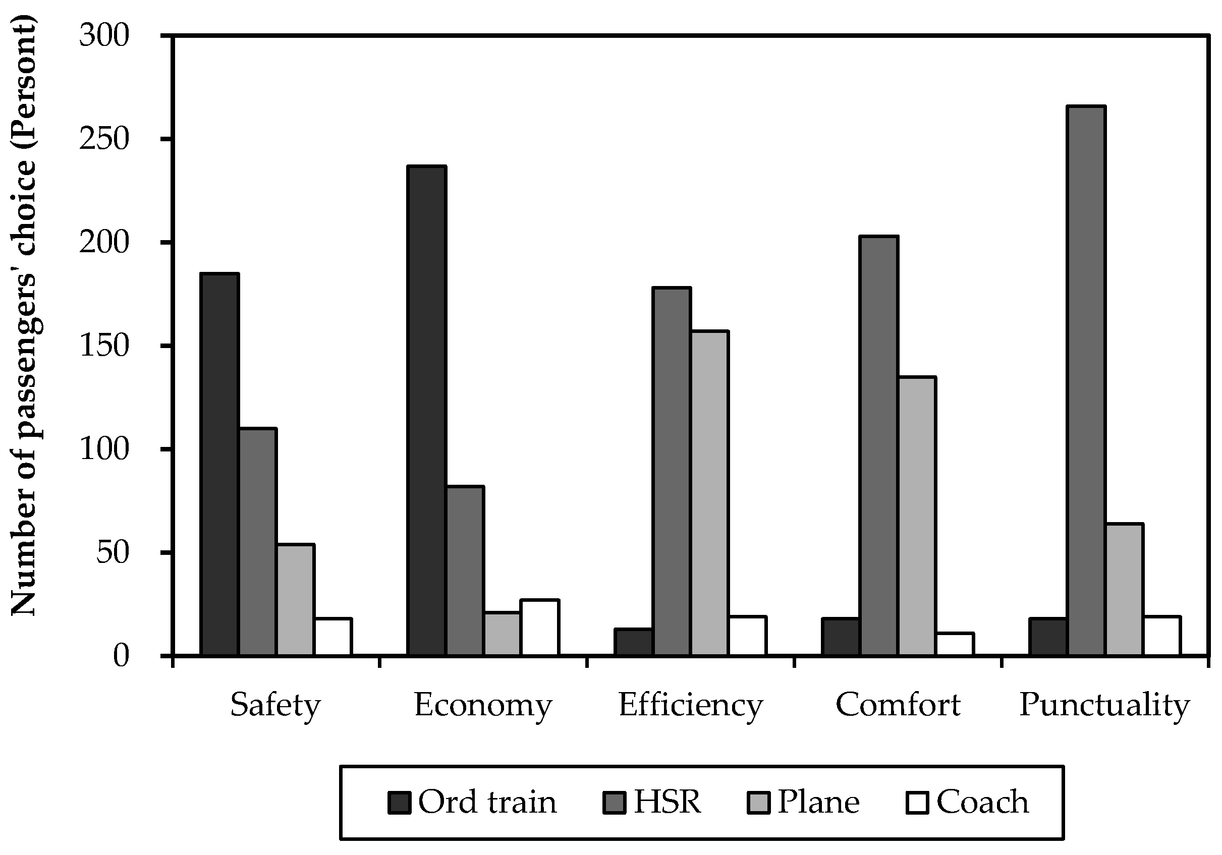
Figure 4.
Relationship between vocation and travel mode choice: (a) Vocation Cluster #1; (b) Vocation Cluster #2; and (c) Vocation Cluster #3.
Figure 4.
Relationship between vocation and travel mode choice: (a) Vocation Cluster #1; (b) Vocation Cluster #2; and (c) Vocation Cluster #3.
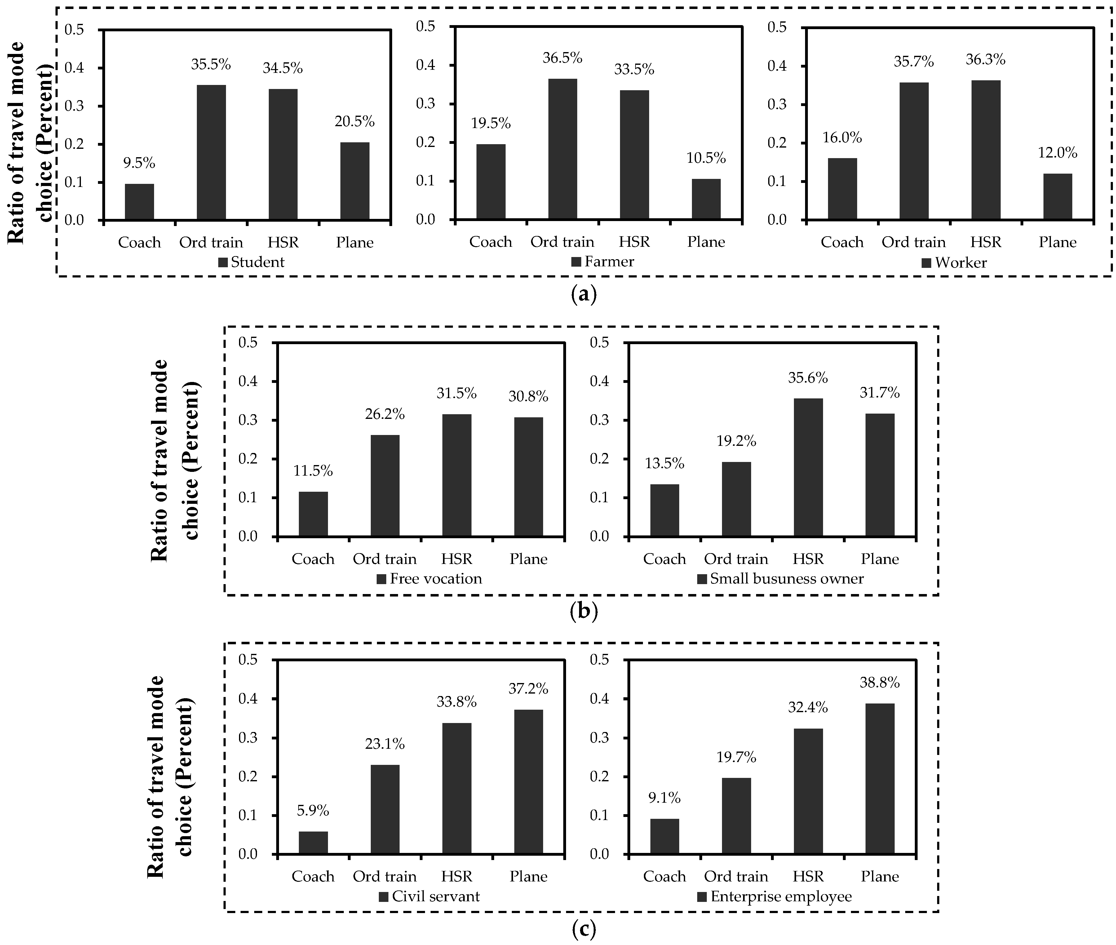
Figure 5.
Relationship between travel mode choice and different importance levels of service preference for economy, comfort, punctuality and efficiency: (a) service demand for economy; (b) service demand for comfort; (c) service demand for punctuality; and (d) service demand for efficiency.
Figure 5.
Relationship between travel mode choice and different importance levels of service preference for economy, comfort, punctuality and efficiency: (a) service demand for economy; (b) service demand for comfort; (c) service demand for punctuality; and (d) service demand for efficiency.

Figure 6.
Relationship between performance satisfaction and travel mode choice: (a) average satisfaction scores of travel modes; and (b) travel mode choice distribution.
Figure 6.
Relationship between performance satisfaction and travel mode choice: (a) average satisfaction scores of travel modes; and (b) travel mode choice distribution.
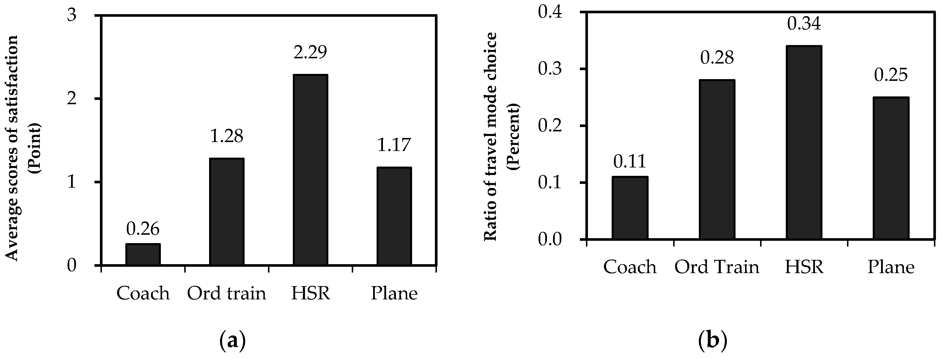
Figure 7.
Travel mode choice in different distance.
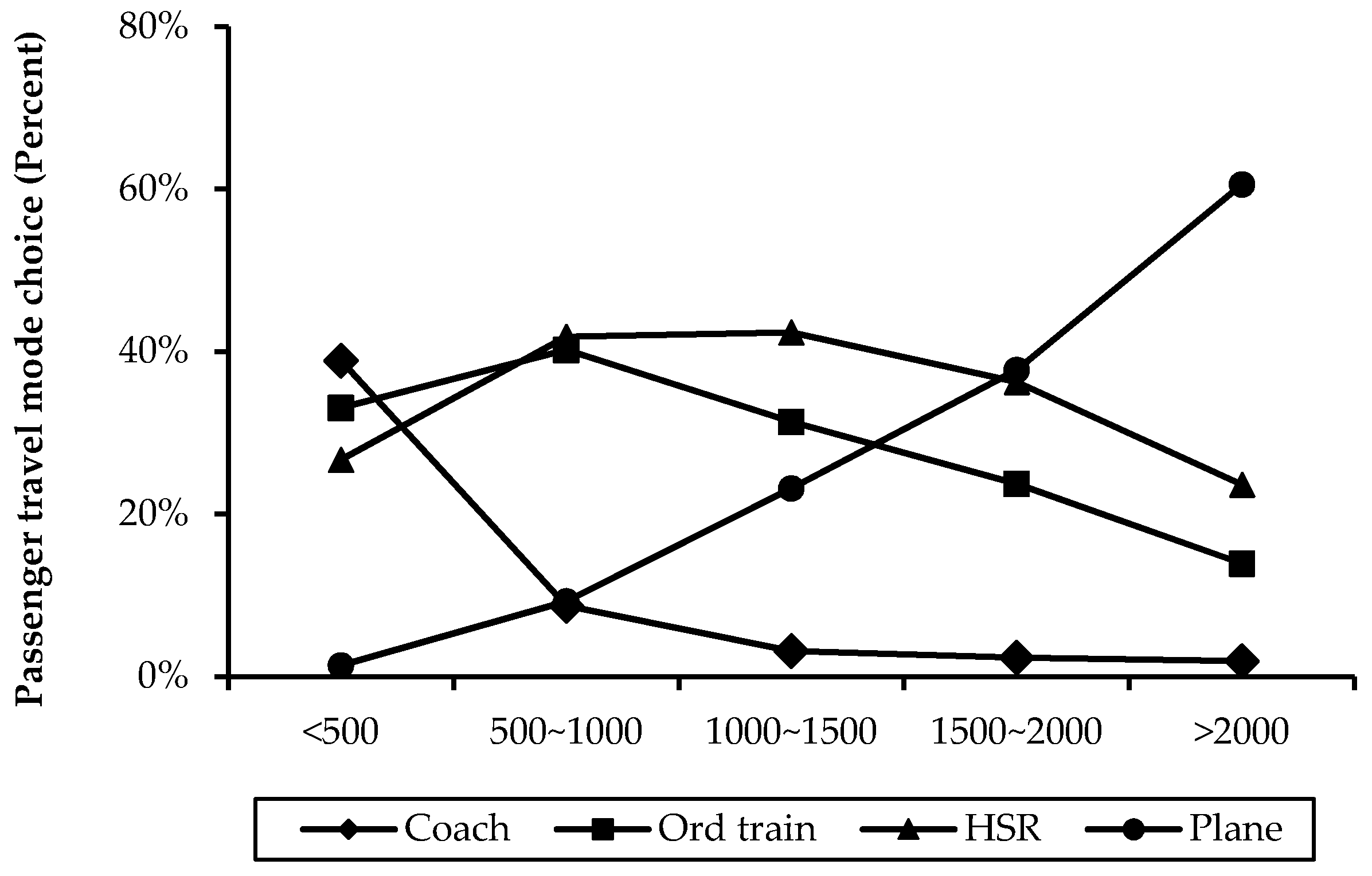
Figure 8.
Structural model of travel mode choice behavior.

Figure 9.
Relationship between income level and different importance levels of service preference for economy, comfort, punctuality and efficiency: (a) service demand for economy; (b) service demand for comfort; (c) service demand for punctuality; and (d) service demand for efficiency.
Figure 9.
Relationship between income level and different importance levels of service preference for economy, comfort, punctuality and efficiency: (a) service demand for economy; (b) service demand for comfort; (c) service demand for punctuality; and (d) service demand for efficiency.

Table 1.
Passengers’ socio-demographic characteristics.
| Variables | Description/Levels | Frequency | Percentage (%) |
|---|---|---|---|
| Gender | Male | 236 | 64.31% |
| Female | 131 | 35.69% | |
| Age | Below 20 | 11 | 3% |
| 20–29 | 176 | 48% | |
| 30–39 | 74 | 20.2 | |
| 40–49 | 70 | 19.1 | |
| Above 50 | 36 | 9.8 | |
| Education level | Low-education | 188 | 51.20% |
| Middle-education | 154 | 42.00% | |
| High-education | 25 | 6.80% | |
| Vocation | Student | 108 | 29.4% |
| Farmer | 20 | 5.4% | |
| Civil servant | 38 | 10.4% | |
| Small business owner | 52 | 14.2% | |
| Worker | 36 | 9.8% | |
| Free vocation | 41 | 11.2% | |
| Enterprise employees | 56 | 15.3% | |
| Others | 16 | 4.4% | |
| Income | Low-income | 293 | 80.00% |
| Middle-income | 44 | 12.00% | |
| High-income | 30 | 8.00% |
Table 2.
Distribution of passengers’ service preference.
| Service Preference Attributes | Most Important | Second Important | Third Important | Forth Important | Least Important | Total |
|---|---|---|---|---|---|---|
| Safety | 285 | 35 | 25 | 19 | 3 | 367 |
| Price | 27 | 125 | 72 | 65 | 66 | 367 |
| Comfort | 25 | 76 | 62 | 104 | 86 | 367 |
| Punctuality | 19 | 80 | 111 | 70 | 105 | 367 |
| Efficiency | 11 | 81 | 75 | 109 | 99 | 367 |
Table 3.
Results of the analysis of variance.
| Variables | Sum of Squares | df | Mean Square | F | Sig | |
|---|---|---|---|---|---|---|
| Passengers’ socio-demographic characteristics | Gender | 0.5 | 1 | 0.5 | 0.5 | 0.48 |
| Education level | 65.5 | 2 | 32.7 | 35.7 | 0.00 * | |
| Vocation | 130.3 | 7 | 18.6 | 20.7 | 0.00 * | |
| Income | 125.7 | 7 | 18.0 | 19.9 | 0.00 * | |
| Service preference attributes | Preference for safety | 12.0 | 4 | 3.0 | 3.2 | 0.12 |
| Preference for price | 196.8 | 4 | 49.2 | 55.9 | 0.00 * | |
| Preference for efficiency | 107.5 | 4 | 26.9 | 29.7 | 0.00 * | |
| Preference for comfort | 146.3 | 4 | 36.6 | 40.9 | 0.00 * | |
| Preference for punctuality | 83.8 | 4 | 21.0 | 23.0 | 0.00 * | |
| Performance satisfaction | Satisfaction of safety | 90.6 | 4 | 22.6 | 24.9 | 0.00 * |
| Satisfaction for price | 57.9 | 3 | 19.3 | 21.0 | 0.00 * | |
| Satisfaction for efficiency | 23.4 | 3 | 7.8 | 8.4 | 0.00 * | |
| Satisfaction for comfort | 28.8 | 3 | 9.6 | 10.4 | 0.00 * | |
| Satisfaction for punctuality | 44.2 | 3 | 14.7 | 16.0 | 0.00 * | |
| Trip attributes | Departure time | 2.1 | 1 | 2.1 | 2.3 | 0.13 |
| Travel distance | 10,007.0 | 4 | 251.8 | 381.6 | 0.00 * | |
* Significant at the 0.01 level.
Table 4.
Passengers’ travel mode choice based on passengers’ personal attributes.
| Independent Variables | Coach | Ordinary Train | HSR | Plane | ||||
|---|---|---|---|---|---|---|---|---|
| N | % | N | % | N | % | N | % | |
| Age | ||||||||
| Below 20 | 12 | 10.9 | 31 | 28.2 | 50 | 45.5 | 17 | 15.5 |
| 20–29 | 201 | 11.4 | 546 | 31.0 | 566 | 32.2 | 447 | 25.4 |
| 30–39 | 81 | 10.9 | 159 | 21.5 | 271 | 36.6 | 229 | 30.9 |
| 40–49 | 85 | 12.1 | 176 | 25.1 | 237 | 33.9 | 202 | 28.9 |
| Above 50 | 27 | 7.5 | 122 | 33.9 | 137 | 38.1 | 74 | 20.6 |
| Education | ||||||||
| Low-education | 250 | 13.3 | 563 | 29.9 | 655 | 34.8 | 412 | 21.9 |
| Middle-education | 136 | 8.8 | 436 | 28.3 | 519 | 33.7 | 449 | 29.2 |
| High-education | 20 | 8.0 | 35 | 14.0 | 87 | 34.8 | 108 | 43.2 |
| Vocation | ||||||||
| Student | 104 | 9.5 | 387 | 35.5 | 376 | 34.5 | 223 | 20.5 |
| Farmer | 39 | 19.5 | 73 | 36.5 | 67 | 33.5 | 21 | 10.5 |
| Civil servant | 23 | 5.9 | 90 | 23.1 | 132 | 33.8 | 145 | 37.2 |
| Small business owner | 70 | 13.5 | 100 | 19.2 | 185 | 35.6 | 165 | 31.7 |
| Worker | 56 | 16 | 125 | 35.7 | 127 | 36.3 | 42 | 12.0 |
| Free vocation | 45 | 11.5 | 102 | 26.2 | 123 | 31.5 | 120 | 30.8 |
| Enterprise employees | 53 | 9.1 | 114 | 19.7 | 188 | 32.4 | 225 | 38.8 |
| Others | 16 | 10.7 | 43 | 28.7 | 63 | 42 | 28 | 18.7 |
| Income | ||||||||
| Low-income | 302 | 11.3 | 879 | 32.8 | 923 | 34.4 | 576 | 21.5 |
| Middle-income | 68 | 11.5 | 121 | 20.5 | 195 | 33.1 | 206 | 34.9 |
| High-income | 36 | 9.0 | 34 | 8.5 | 143 | 35.8 | 187 | 46.8 |
| Total | 406 | 11.1 | 1034 | 28.2 | 1261 | 34.4 | 969 | 26.4 |
Table 5.
Summarization on travel modes’ competitiveness and relevant suggestions.
| Travel Mode | Competitive Travel Distance Scope | Performance Features | Target Passenger Groups | Relevant Suggestions |
|---|---|---|---|---|
| Coach | <500 km. | low satisfaction degree of service performances. | lack of competitiveness among all groups. | (1) vigorously improving service quality; (2) enhancing the highway construction between cities to provide proper environment for haul business in relatively short distance. |
| Ordinary train | 500–1000 km. | low travel expense; high satisfaction degree of safety performance; low satisfaction degree of the performances on efficiency, comfort and punctuality. | low-income; student, farmer and worker. | (1) providing diversified service; (2) broadening the competitive distance scope to longer distance. |
| HSR | highly competitive over each distance scope, especially within 500–1000 km. | high travel expense; satisfied performances on safety, efficiency, comfort and punctuality. | highly competitive among almost all groups. | (1) taking economic incentive strategies, such as ticket discount and bonus points; (2) improving the construction of branch lines in the middle-long distance. |
| Plane | highly competitive in relatively long distance, especially over 2000 km. | high travel expense; low satisfaction degree of punctuality performance; satisfied performances on comfort and efficiency. | high-income; civil servant, enterprise employee. | (1) improving punctuality performance to ensure reliability; (2) properly taking economic incentive strategies. |
Table 6.
Definition of variables in SEM models.
| Variables | Coding of Input Value | ||
|---|---|---|---|
| Latent Variable | Observed Variable | Description | |
| Personal attributes | Age | Passenger’s age group. | 1→ Below 20 |
| 2→ 20–29 | |||
| 3→ 30–39 | |||
| 4→ 40–49 | |||
| 5→ Above 50 | |||
| Education | Passenger’s education level. | 1→ high school or under | |
| 2→ bachelor degree | |||
| 3→ master degree or above | |||
| Vocation | Passenger’s vocation classification. | 1→ student | |
| 2→ farmer | |||
| 3→ civil servant | |||
| 4→ small business owner | |||
| 5→ worker | |||
| 6→ free vocation | |||
| 7→ enterprise employees | |||
| 8→ others | |||
| Income | Passenger’s income level. | 1→ <6000 RMB | |
| 2→ 6000–10,000 RMB | |||
| 3→ >10,000 RMB | |||
| Service preference attributes | P_Economy/ | Passenger’s ranking on preference about safety, economy, efficiency, comfort and punctuality for long distance travel. | 1→ the least important |
| P_Efficiency/ | 2→ the forth important | ||
| P_Comfort/ | 3→ the third important | ||
| P_Punctuality | 4→ the second important | ||
| 5→ the most important | |||
| Performance satisfaction attributes | S_Safe/ | Passenger’s satisfaction to the most competitive travel mode in safety, economy, efficiency, comfort and punctuality respectively. | 1→ coach |
| S_Economy/ | 2→ ordinary train | ||
| S_Efficiency/ | 3→ HSR | ||
| S_Comfort/ | 4→ plane | ||
| S_Punctuality | |||
| / | Distance | The assumptive travel distance of long distance travel. | 1→ <500 |
| 2→ 500–1000 | |||
| 3→ 1000–1500 | |||
| 4→ 1500–2000 | |||
| 5→ >2000 | |||
| / | Travel mode choice | Passenger’s mode choice under a certain assumptive travel time and travel distance. | 1→ coach |
| 2→ ordinary train | |||
| 3→ HSR | |||
| 4→ plane | |||
Table 7.
Results of Testing Model 3.
| Equations | Observed Variables | Latent Variables | Estimate | S.E. | t-Value | p |
| Measurement equation for exogenously latent variable (personal attributes) | Income | Personal attributes | 1 | *** | ||
| Vocation | Personal attributes | 4.776 | 0.26 | 18.364 | *** | |
| Education level | Personal attributes | −0.878 | 0.051 | −17.273 | *** | |
| Age | Personal attributes | 2.814 | 0.145 | 19.339 | *** | |
| Measurement equation for exogenously latent variable (service preference and performance satisfaction) | P_Punctuality | Service preference | −0.832 | 0.078 | −10.629 | *** |
| P_Comfort | Service preference | −0.974 | 0.105 | −9.291 | *** | |
| P_Efficiency | Service preference | −0.272 | 0.033 | −8.200 | *** | |
| P_Economy | Service preference | 1 | ||||
| S_Punctuality | Satisfaction | 1 | ||||
| S_Comfort | Satisfaction | 0.925 | 0.125 | 7.409 | *** | |
| S_Efficiency | Satisfaction | 0.425 | 0.063 | 6.692 | *** | |
| S_Economy | Satisfaction | 0.208 | 0.037 | 5.614 | *** | |
| S_Safety | Satisfaction | 0.567 | 0.082 | 6.953 | *** | |
| Equations | Endogenously Latent Variables | Exogenously Latent Variables | Estimate | S.E. | t-Value | p |
| Structural equation for travel mode choice mechanism in long-distance | Service preference | Personal attributes | −1.13 | 0.09 | −12.544 | *** |
| Satisfaction | Personal attributes | 0.059 | 0.01 | 5.899 | *** | |
| Mode choice | Service demand | −0.669 | 0.061 | −10.947 | *** | |
| Mode choice | Satisfaction | 0.532 | 0.062 | 8.583 | *** | |
| Mode choice | Travel distance | 0.362 | 0.009 | 40.493 | *** | |
| Mode choice | Departure time | 0.042 | 0.025 | 1.67 | 0.095 | |
| Mode choice | Personal attributes | 0.557 | 0.098 | 5.697 | *** |
*** means the estimate was significant at the 95% confidence level.
Table 8.
Effects of personal attributes on travel mode choice.
| Latent Variables | Observed Variables | Direct Effects | Indirect Effects | Total Effects |
|---|---|---|---|---|
| Personal Attributes | 0.16 | −0.59 × −0.36 + 0.20 × 0.27 = 0.27 | 0.43 | |
| Age | 0.11 | 0.71 × 0.27 = 0.19 | 0.30 | |
| Education level | 0.08 | 0.48 × 0.27 = 0.13 | 0.20 | |
| Vocation | 0.09 | 0.55 × 0.27 = 0.15 | 0.23 | |
| Income | 0.07 | 0.44 × 0.27 = 0.12 | 0.19 | |
Table 9.
Fit statistics for structural equation models.
| Fix Index | SEM Models | Criteria of Acceptable Fit |
|---|---|---|
| Chi-square | 86.785 | Smaller values |
| df | 75 | |
| p-value | 0.016 *** | >0.05 |
| GFI | 0.997 | >0.9 |
| AGFI | 0.994 | >0.9 |
| CFI | 0.998 | >0.9 |
| NFI | 0.988 | >0.9 |
| RMSEA | 0.007 | <0.05 |
*** means the estimate was significant at the 95% confidence level.
© 2017 by the authors. Licensee MDPI, Basel, Switzerland. This article is an open access article distributed under the terms and conditions of the Creative Commons Attribution (CC BY) license (http://creativecommons.org/licenses/by/4.0/).
Share and Cite
MDPI and ACS Style
Wang, Y.; Yan, X.; Zhou, Y.; Xue, Q. Influencing Mechanism of Potential Factors on Passengers’ Long-Distance Travel Mode Choices Based on Structural Equation Modeling. Sustainability 2017, 9, 1943. https://doi.org/10.3390/su9111943
AMA Style
Wang Y, Yan X, Zhou Y, Xue Q. Influencing Mechanism of Potential Factors on Passengers’ Long-Distance Travel Mode Choices Based on Structural Equation Modeling. Sustainability. 2017; 9(11):1943. https://doi.org/10.3390/su9111943
Chicago/Turabian StyleWang, Yun, Xuedong Yan, Yu Zhou, and Qingwan Xue. 2017. "Influencing Mechanism of Potential Factors on Passengers’ Long-Distance Travel Mode Choices Based on Structural Equation Modeling" Sustainability 9, no. 11: 1943. https://doi.org/10.3390/su9111943
Note that from the first issue of 2016, this journal uses article numbers instead of page numbers. See further details here.