Spatial–Temporal Modeling for Regional Economic Development: A Quantitative Analysis with Panel Data from Western China


1
School of Economics and Management, Chang’an University, Middle-section of Nan’er Huan Road, Xi’an 710064, China
2
School of Civil Engineering, Chang’an University, No.161, Chang’an Road, Xi’an 710061, China
3
Assistant Professor, Bert S. Turner Department of Construction Management, Louisiana State University, 3315D Patrick F. Taylor Hall, Baton Rouge, LA 70803, USA
*
Authors to whom correspondence should be addressed.
Sustainability 2017, 9(11), 1955; https://doi.org/10.3390/su9111955
Submission received: 17 July 2017
/
Revised: 16 October 2017
/
Accepted: 16 October 2017
/
Published: 27 October 2017
Abstract
:The objective of this research is to analyze regional economic difference and explore the influencing factors, which would eventually provide an effective foundation to narrow the regional economic differences. In this paper, a new regional economic difference model is established considering the interactions between the spatial weight and human capital and foreign direct investment (FDI). With the panel data from twelve western provinces in China, the empirical research is conducted by adopting feasible generalized least squares (FGLS) fixed effects model. The preliminary results show that: (1) the spatial spillover effect of human capital and FDI is significant to the formation of regional economic difference; and (2) the total capital formation, government expenditure, FDI, human capital and patent application authorization are positively correlated with GDP growth per capita, while the number of medical institutions is negatively correlated with GDP growth per capita. In addition, the robust test is carried out for validation by using the filter variable method, spatial lag model and spatial error model. The robustness test results show that the results of the FGLS fixed effects model are validated by the filter variable method. The other two robust test results show that: (1) the total capital formation and the fixed asset investment is of 99.9% significance, which represents that they play a key role in the formation of economic development difference; and (2) the coefficients’ symbols of the other variables are consistent with the FGLS fixed effect model but a little different on the significances, which enhance the effectiveness of the proposed regional economic difference model.
1. Introduction
Economic inequality has become an increasingly prominent global issue for economic development, especially in underdeveloped regions or special regions of developing countries [1,2], for example, the western regions of China. A Western Development Strategy was proposed in 2000 by Chinese government aiming to overcome the economic backwardness and better support the economic development of western regions [3,4]. Although this policy has promoted the regional economic development to a certain extent, the economic development difference in the west regions has not stopped enlarging. This creates the phenomenon of “the strong get stronger and the weak get weaker”. The current economic development within western China remains significantly unbalanced, and, to some degree, it is becoming even worse than before. For example, in the underdeveloped areas such as Tibet, Gansu and other provinces, people are suffering a low standard of living, and this seriously affects the social harmony and stability, blocks the process of regional modernization, and influences the efficiency of regional economic development. All of these problems have greatly affected the sustainable and healthy development of Chinese economy [5]. The key of alleviating current situation is to identify the top influencing factors that affects regional economic difference in western China. Currently, regional economic difference in China is a popular research topic [6,7,8,9], and many studies [10,11,12,13] have been reported. For example, Peng [10] analyzed the spatial–temporal evolution characteristics of three regional economic differences of eastern and western China, and other regions of China have been studied similarly by other researchers [11,12,13]. Yang [12] used Henan province as an example to explore the influencing factors of regional economic growth difference, and concluded that location condition, capital condition, and industrial structure are the important factors influencing regional economic growth difference. Liu et al. [13] analyzed the panel data from 1987 to 2017 and verified the transportation infrastructure had a significant positive effect on Chinese economic growth. However, little research has been done to analyze the economic difference of western China with the latest panel data, and to recognize the top impact factors not only at the theoretical level but also at the policy implementation level. Thus, there is a need of identifying the influencing factors of regional economic development in western China, such as whether the Western Development Strategy and industrial isomorphism are the significant influencing factors, whether the western region still relies on fixed asset investment to drive economic development or not, etc. The research objectives of this paper are to realize this need, analyze the important influencing factors of regional economic development using the proposed spatial–temporal model with the latest panel data [6], and provide corresponding suggestions to sustain the economic development in western China.
In this paper, the authors established a regional economic difference model based on spatial–temporal effect, analyzed the important influencing factors of regional economic difference by using the feasible generalized least squares (FGLS) fixed effect model, and validated it through robustness testing. This study first analyzed the influencing factors of regional economic difference, compared with the existing literature, and added new variables including the number of universities and medical institutions. Meanwhile, this research introduced industrial isomorphism, population density, and the dummy variables of Western Development Strategy as control variables. Secondly, based on generic spatial–temporal model [14,15], considering the interactions between spatial weights, human capital and foreign direct investment, the authors proposed an innovative regional economic difference model, and applied the FGLS fixed effect model to identify the top influencing factors to reduce the regional economic difference. Finally, the robustness testing was conducted by using the filter variable method, spatial lag model, and spatial error model [15]. The main contributions to the body of knowledge are: (1) the variables considered in this research are comprehensive compared with the existing research, while the space weight matrix is applied to FGLS fixed effects model [15]; (2) the proposed approach integrates FGLS fixed effects model and the spatial–temporal effect, which could overcome the shortcoming of lacking the individual spatial correlation and reduce the endogenous in the traditional model [14]; and (3) the research results provide a good reference for the regional economic difference analysis in the similar regional economic and other developing countries.
Following the Introduction, Section 2 analyzes the influencing factors of regional economic difference through literature review. In Section 3, an innovative regional economic difference model based on spatial–temporal effect was proposed. Section 4 introduces a case study analyzing the panel data from western China to explore the regional economic difference, and applies the FGLS fixed effects model to identify the influencing factors. Section 5 integrates the filter variable method, the spatial lag model and the spatial error model to conduct the robustness testing. Section 6 discusses how to respond to the influencing factors to form a reasonable space development pattern, gradually reduce regional economic development differences, and promote the sustainable development of Western China. Section 7 summarizes the conclusions of this study and discusses the limitations.
2. Literature Review
The difference of regional economic development can be explained in two ways. One is from the perspective of the spatial effect between regions, which mainly refers to the impact of industrial agglomeration, cluster and isomorphism on regional economic growth. The other is from the perspective of regional internal analysis, and the influencing factors of economic development cover not only fixed assets, human capital, scientific and technological innovation, and foreign investment, but also related policies and development strategies.
2.1. Spatial Effects between Regions
For example, Boschma [16,17] applied the evolution model to analyze the positive correlation between industrial agglomeration and economic development. Yu [18] conducted the principal component analysis to analyze the importance of industrial agglomeration in a regional economy, and provide a foundation for local government to take effective policies to promote economic growth. Niu [19] introduced panel data model and GIS spatial analysis method to realize the positive correlation between regional expansion and economic growth. Xu [20] adopted the cluster analysis and GIS technology to analyze the structural characteristics of regional economic difference, and stated that the economic development level is directly related to the regional locations. Chen and Zhu [21] studied the variation coefficient method and spatial autocorrelation to measure the spatial pattern of regional economy in China, and concluded that GDP per capita at provincial, local, and country level had significant spatial autocorrelation.
2.2. Internal Region
From the global perspective, Galazova assessed the role of knowledge innovation in economic growth in the current economic situation [22]. Crescenzi used time fixed effects model to explore the relationship among the three policies of EU and regional economic growth, and concluded that the three policies promoted the economic growth, but regional policy played the main role [15]. Choi found that there is a certain spatial correlation between regional economic development and land utilization [23]. Kim analyzed the panel data for the correlation regression analysis, and found that the government consumer expenditure showed the obvious negative effect on the economic growth [24,25]. Berthlemy [26] and Fleisher [27] stated that the root causes of the regional economic development difference were human capital and FDI. In addition, Shim [28] used the fixed effect model to analyze the promoting impact of infrastructure construction on regional economic growth.
From Chinese regional economic perspective, Dai [29] analyzed the influencing factors of regional economic difference within three northeastern provinces, and found that the impact of industrial structure, investment and marketization level on regional economic difference were significant. Zhang [30], Wu [31], and Li [32] argued that indicators including natural and geographical conditions, human capital, policy inclination, innovation ability and financial expenditure were important influencing factors on regional economic difference. Kong [33] used the vector autoregressive model to analyze the fixed asset investment as an important factor to influence regional economic difference. Xu and Liao [33] analyzed the relationship among final consumption expenditure, total capital formation, and actual GDP, and this uncovered that the total capital formation had an obvious short-term effect on economic development as well as a weak long-term effect.
Many researchers focus on endogenous factors, such as policy expenditure, total capital formation, fixed asset investment, financial industry agglomeration, etc., to generate their contribution rate on economic growth. However, little research concentrated on the difference of regional economic development with the comprehensive consideration industrial structure, Western Development Strategy, endogeneity, and spatial factors in western China. In this paper, the proposed model integrated the spatial weight factor into a generic spatial–temporal model, which is an innovative approach of analyzing the economic difference of western China.
3. The Proposed Regional Economic Difference Model
3.1. General Spatial–Temporal Model
There are three regional spatial economic difference models [34], which are spatial–temporal data model, spatial lag model, and spatial error model. Regional economic difference is divided into three categories: absolute difference, relative difference, and comprehensive difference. In this paper, it is referred as the absolute difference. In the following sections, the proposed model was introduced on how it can be used to analyze the influencing factors, and then the model robust test was conducted by using the filter variable method, spatial lag model, and spatial error model.
The general form of spatial–temporal data models is shown in Formula (1) [14]:
where is the interpreted variable, is the explanatory variable, stands for time, represents different individual, and is random disturbance item. The coefficients in the model can be different with the different of individual and time, and thus the generic model can reflect the influence of the neglected individual factors and time factors in spatial–temporal process.
3.2. Extended Application of General Model
Based on the abovementioned model, this study integrated the research framework from Zhang [30], Wu [31], and Li [32]; considered the economic difference influence variables in recent research on Chinese western economic; and built the linear model, as shown in Formula (2):
is the natural logarithm of GDP per capita at the end of the year; is the capital matrix; is the government expenditure; is the external environment; is the basic facility matrix; is the knowledge innovation matrix; is the spatial lag variable matrix; is the control variable matrix; is a specific error; represents the regions; and represents the years. Detailed explanations are shown as follows:
(1) Natural logarithm of GDP per capita () in the western region at the end of each year
is as an interpreted variable, which is the true reflection of regional economic performance, using the natural logarithm of the actual value of GDP per capita to identify, i.e., . GDP refers to the final outcome of the production activities of all permanent units of a region calculated by the market price in a certain period. The reason for choosing GDP per capita is that it can eliminate the regional difference on the aspect of population and land area, and can accurately reflect the real economic development rate of the region [35].
(2) Capital matrix
The capital here refers to the financial capital. Two indicators, total capital formation (TCF) and fixed asset investments (FAI), are introduced to measure the capitals’ impact on the economic differences [33,36]. Total capital formation refers to the net amount calculated by subtracting the disposed fixed assets and inventories within a certain period from the permanent unit. The fixed asset investments are the work and cost in the form of money for building and purchasing the fixed assets in the certain period.
(3) Government expenditure
Government spending refers to use the fiscal expenditure (FE) to measure the government impact on economic differences, wherein it refers to the government investment expenditure [32]. The fiscal expenditure includes the expenses in general public service, national defense, public security, education, science and technology, cultural sports and media, social security employment, medical and health, environmental protection, urban and rural community affairs, agricultural and forestry water affairs, transportation, etc.
(4) External environment
Economic globalization has great impact on the rapid development of the enterprises. Therefore, the external economic environment is particularly important. This research used the foreign direct investment (FDI) as an indicator of the external economic conditions [26]. FDI refers to foreign enterprises and economic organizations or individuals, in accordance with China’s relevant policies and regulations, using cash, technology, etc. to open foreign-owned enterprises in China, and organize joint ventures, cooperative ventures or cooperation in the development of resources investment with the domestic enterprises or economic organizations; and the funds borrowed by the enterprise from abroad under the total project investment approved by the relevant government departments.
(5) Infrastructure matrix
Infrastructure is the facility that provides public services for social production and residential life, and it includes transportation, water and electricity supply, commercial services, landscaping, cultural education, medical and health services, municipal public works facilities, public life services facilities, etc.
Due to limited data access, this research used three main indicators to interpret the conditions of infrastructure from transportation, cultural education, and medical and health services aspects: railway line length (RLL) [37,38], the number of college and universities (OHS) and the number of medical institutions (MI).
(6) Knowledge innovation matrix
This research used the following two variables to explain the knowledge Innovation matrix: human capital (HC) [30,39] and the number of domestic patent authorization (PA). Human capital refers to the average amount of students for each 100,000 populations in the university, which is shown as:
The number of the patent authorization represents the regional technical innovation ability [31]. Patent is the abbreviation of patent right. When inventions are qualified after examination, the Patent Office, in accordance with patent law, grant inventors and designers the exclusive rights of the invention including inventions, utility models, and exterior designs.
(7) Spatial lag variable
There are three methods of computing the weight matrix [18], adjacency matrix, geographical distance matrix, and economic distance matrix. The weight matrix in this research is calculated following the criterion of adjacency matrix, which is defined as follows:
The spatial lag variable refers to use the spatial weight matrix multiplies the human capital and foreign direct investment, respectively, which could reduce the time and space error as well as the errors caused by the difference between regions.
(8) Control variables
There are three control variables: Krugman index, population density (PD), and a policy dummy variable.
Firstly, this research applied the Krugman index to explain the industrial isomorphism. Krugman industrial division index can be used to measure the overall difference of industrial structure between regions. Krugman index between two regions is shown as follows:
where represents the industry proportion of the whole industry in region, and represents the industry proportion of the whole industry in region. As for Chinese statistical year book, the industry is divided into primary, secondary, and the tertiary industry. The sum of these three industrial added values represents the regional gross domestic product (GDP). When region and j have the same industrial structure, Krugman index is zero. When the two-industrial structures are completely different, Krugman index is two.
Due to the scope of this study of analyzing 12 provinces in the western China, it is certainly a burden to generate the Krugman index between two regions. As a simple and effective method referenced in the existing research [18], we applied the average value of the sum of the Krugman index calculated by region and the remaining 11 regions to measure the industrial isomorphism between the region and the rest of the region. The second control variable is population density (PD). To solve the difference of compared base caused by the regional population, this research used the population density as control variable to increase the interpretation of remaining variables. The third control variable takes the consideration of policy factors as dummy variable. We choose the Western Development Strategy (DWEST) as the policy dummy variable. DWEST is implemented after the year 2000, Thus, before the year 2000, policy dummy variable DWEST is 0; after the year 2000, the policy dummy variable DWEST is 1 [18]. As a summary, the above influencing factors are listed in Table 1.
4. Empirical Results
4.1. Data Collection
This research collected panel data of 1994 to 2015 from National Bureau of Statistics (NBS) of the People’s Republic of China [44] (http://www.stats.gov.cn/). According to the region division of Chinese government, the western region of China includes 12 provinces, autonomous regions and municipalities, and they are Sichuan, Yunnan, Chongqing, Shaanxi, Guizhou, Tibet Autonomous Region, Gansu, Qinghai, Ningxia Hui Autonomous Region, Inner Mongolia, Xinjiang Autonomous Region, and Guangxi Autonomous Region. The panel data include 12 provincial cross-section data, and a time series from 1994 to 2015.
Table 2 shows the demographics description of the above 15 indicators corresponding to 12 regions in 22 years. is calculated by using adjacency criteria of 12 western regions.
Table 2 shows that different regions have different variables across the year. There are many big gaps between minimum and maximum, such as for patent authorization with minimum 2 and maximum 64,953. The standard deviations of some variables are relatively high. For example, the standard deviation of FDI is 15,249.63, which indicates that there is fluctuation for FDI and the external invest environment across the 22 years.
4.2. Regional Economic Difference Analysis
According to the data of GDP per capita from 1994 to 2015 in western China, there is a rapid development in recent years, especially after the implementation of Western Development Strategy in 2000. However, with the overall economic rapid development, internal regional economic difference begins to increase simultaneously.
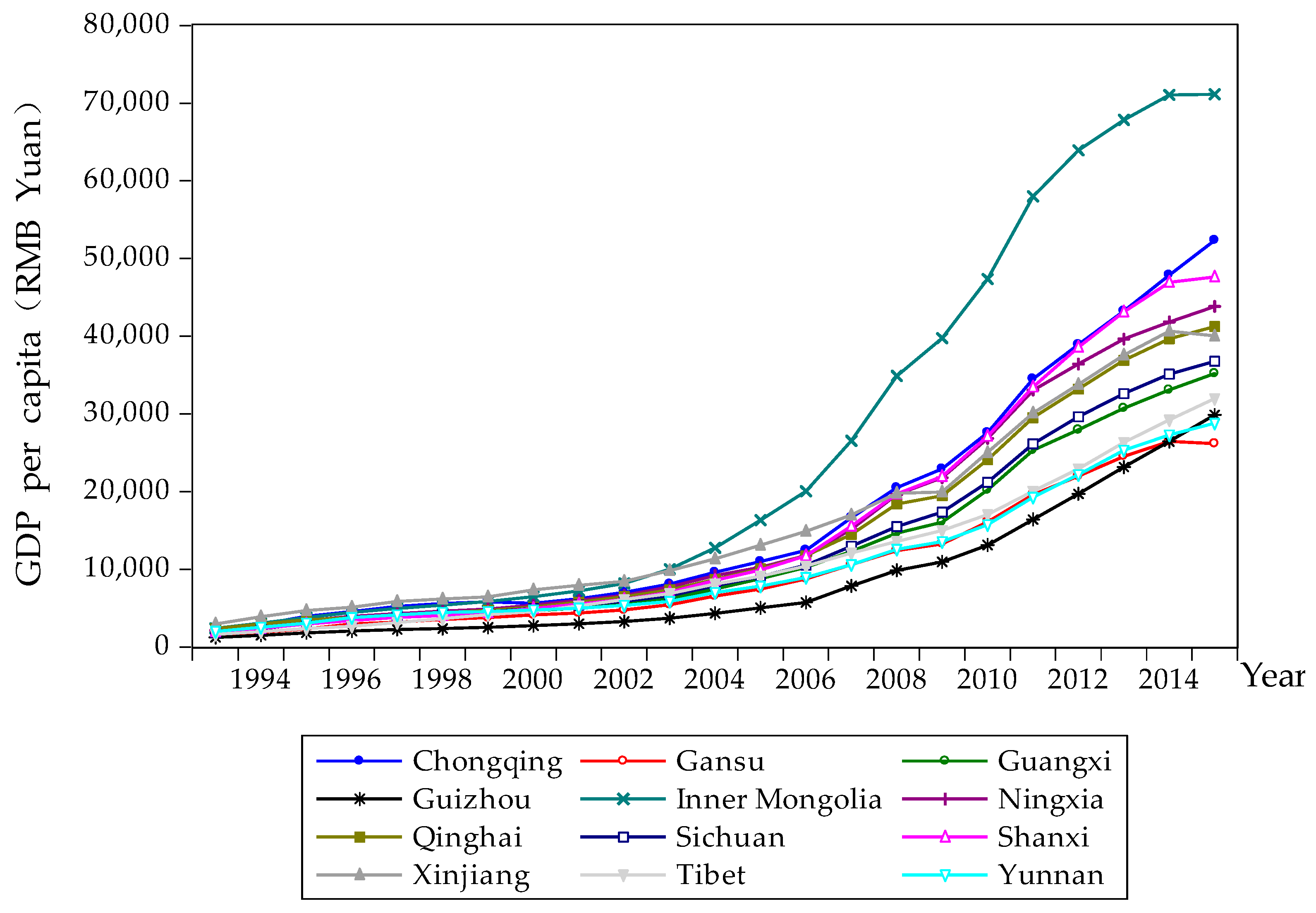
Figure 1 shows that there is almost no difference for GDP per capita in the 12 western regions in 1994. There is a slight growth from 1994 to 2000. After 2000, there is a significant increase in GDP per capita, mainly due to the Western Development Strategy aiming at western economic growth. The fastest economic growing region is Inner Mongolia, Specifically, GDP per capita in both Guizhou and Gansu are the lowest two in 2014; meanwhile, Guizhou has been the lowest before 2014. In addition, on GDP per capita in 2015, there are three regions varying from 20,000 to 30,000, four regions between 40,000 and 50,000, one region between 50,000 and 60,000, and one region over 70,000. It is easy to observe that there is a gradually increasing difference within 12 regions. Thus, it is a practical need to analyze the influencing factor of regional economic difference, such as the long- or short-term impacts of Western Development Strategy. Figure 2 shows that southwestern China lists at the end of GDP per capita, which should become the focus of future economic development difference. The dynamic trend of Krugman indices is shown in Figure 3.
There is an inverse relationship between Krugman index and industrial isomorphism. The smaller the Krugman index is, the greater the industrial isomorphism is, and the smaller the industrial labor division is. Figure 3 shows the Krugman index of southwestern region and Tibetan have always been higher than the other provinces, but southwestern China and Tibetan show a declining trend from 0.53 in 1994 to 0.211 in 2015. In addition, Krugman index of the other provinces stay at the same level, ranging from 0.1 to 0.3. For example, the minimum Krugman index is 0.135, and its maximum is 0.271 in Guizhou. Figure 4 shows that there is a small fluctuation scope from 0.1 to 0.22 for five northwestern provinces. For example, a minimum Krugman index is 0.103 in Gansu, and the maximum in Xinjiang is 0.199. Figure 5 shows the Krugman index comparison among southwest, northwest, Inner Mongolia and Guangxi. In 1994, the minimum Krugman index is 0.124 in Guangxi, and the maximum Krugman index is 0.224 in southwestern China. However, with the recent development, the gap has been narrowed from the minimum 0.148 to the maximum 0.157 in 2015. It can be seen that the western regional industrial isomorphism is gradually increasing, which will result in the decreasing product value and cause the increasing internal vicious competition. It is a clear signal that the enterprise could not benefit from a scaled economic, and the similar industrial isomorphism will eventually hinder economic development.
4.3. Influencing Factors Analysis of Regional Economic Difference
4.3.1 Moran’s I Index Calculation
The Moran’s I index is used to measure the global spatial autocorrelation, reflecting the similarity of spatial adjacency or spatial proximity of the regional unit [28,45,46]. Its range is −1 to 1, and a value closer to 1 indicates more significant spatial positive correlation. This research takes the human capital of west region as an example and carries out the Moran’s I computation. The time series is 1994 to 2015. The Moran’s I is used to determine whether the human capital has spatial spillover, which proves the rationality of introducing the spatial weight matrix.
Moran’s I was generated using Formula (6),
where represents the deviation between and its mean , is the space weight between and , and n is the number. is the aggregation of all spatial weights, which is shown as Formula (7),
is calculated as the following Formula (8),
where
This research used stata13.0 software to calculate the global Moran’s I of western regional human capital shown in Formula (6) from 1994 to 2015; the results are shown in Table 3.
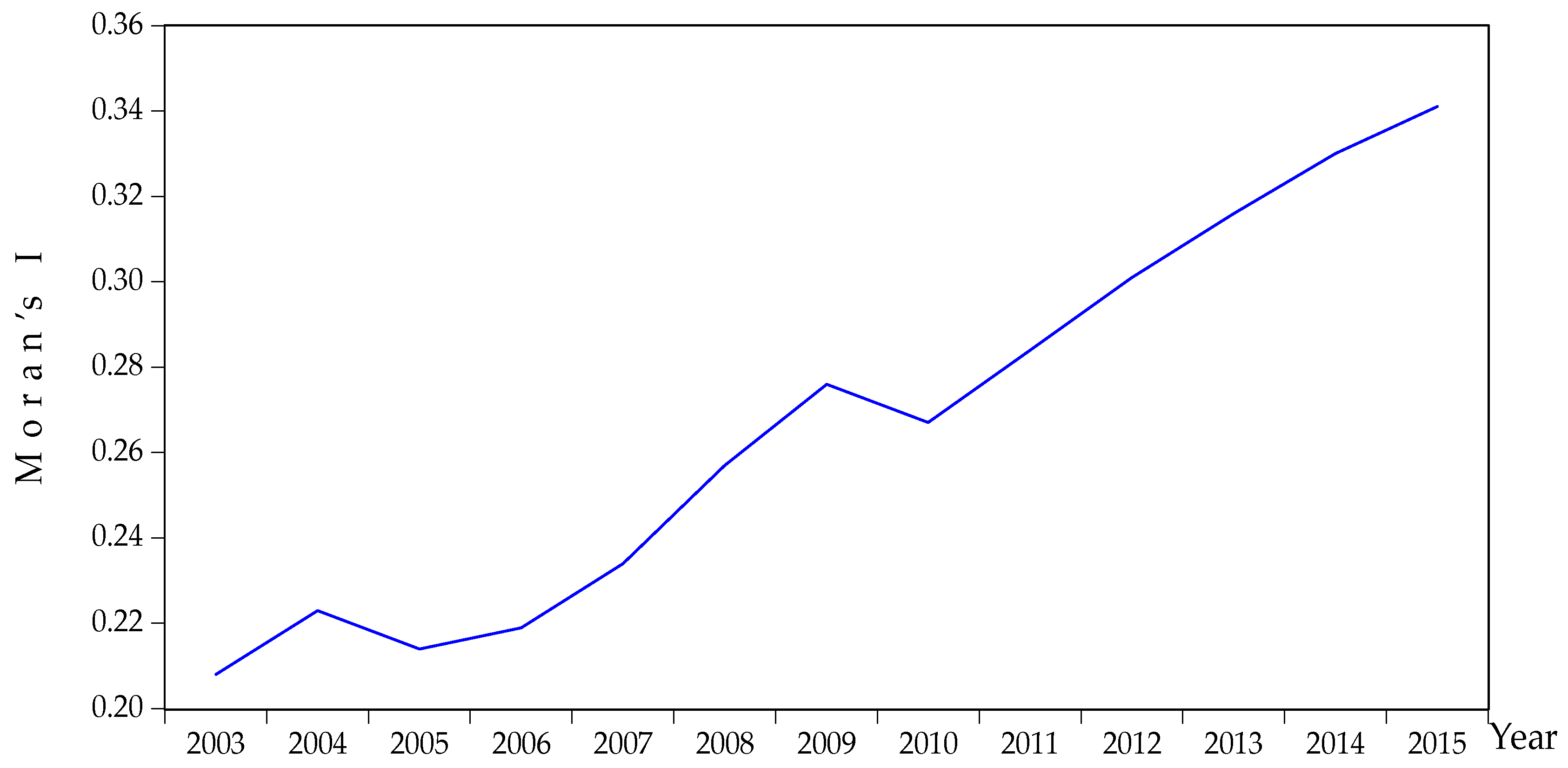
In Table 3, the global Moran’s I of human capital is positive from 1994 to 2015, but the Moran’s I did not pass 95% significance test before 2003, but the Moran’s I did pass 95% significance test after 2003. The following is the trend chart of Moran’s I of Human capital after 2003.
In Figure 6, the Moran’s I of human capital is more than 0.2, and it has a rising trend with time, which indicates that the foreign exchange of students is increasingly frequent, the human capital has significant space spillover effect, and the human capital of different regions are significantly positively interrelated.
Taking 2003 and 2015 as examples, human capital spatial distribution maps were made.
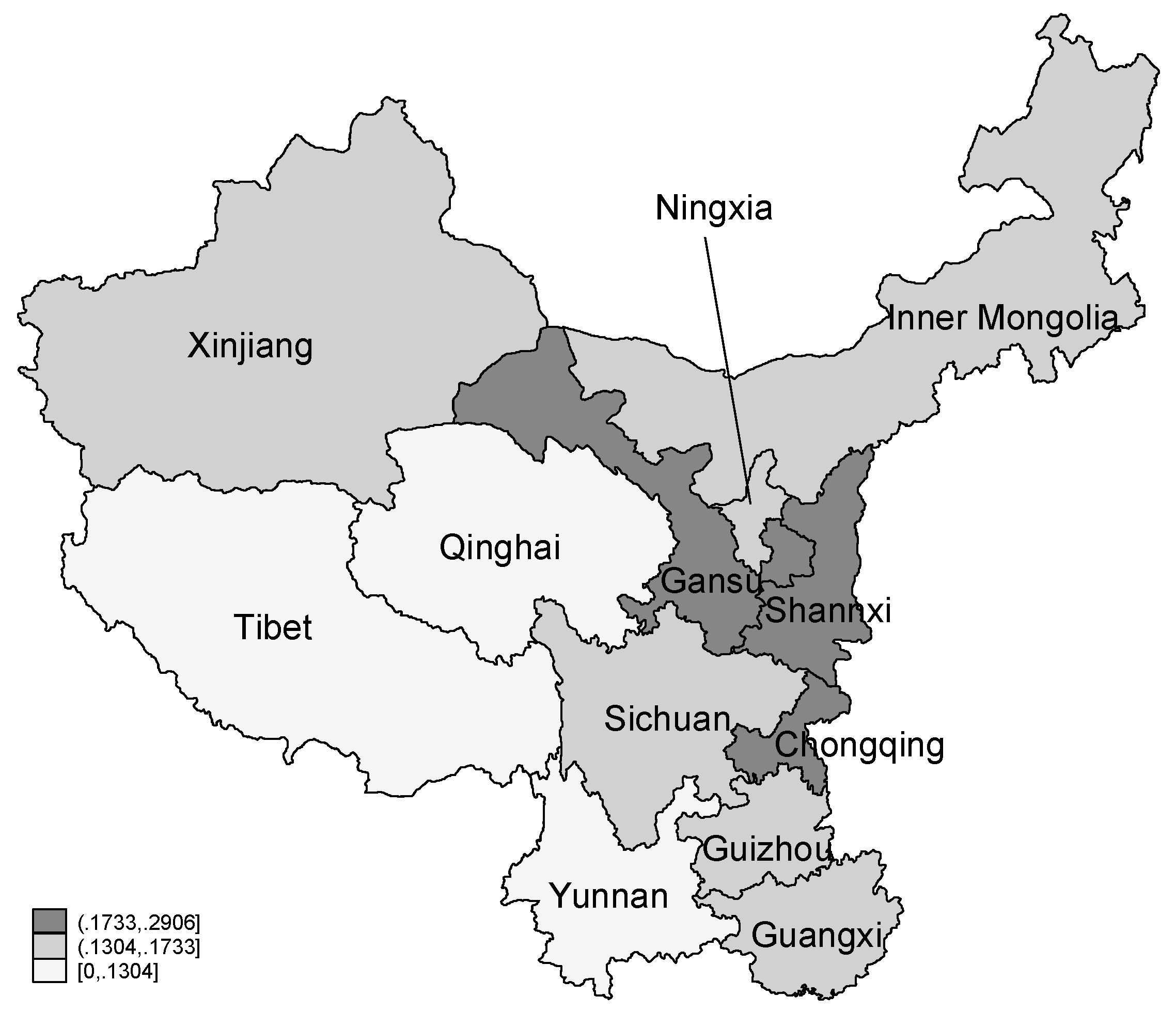
As can be seen in Figure 7 and Figure 8, human capital has more and more obvious spatial spillover effect as time goes by, the closer the region is to the center, the higher the human capital is (Figure 7 and Figure 8 only show the western regions of China, while the eastern and central regions in China are not included). Shaanxi and Chongqing, compared to the other regions in the west, have more geographical advantages and more neighbor provinces. They have greater probability to attract students and to send students out, so the human capital is relatively high.
In summary, in the analysis of regional economic development differences in the western region, the space influence should not be neglected, thus the introduction of space weight matrix is necessary.
4.3.2. Hausman Test
If the possibility of Hausman test is less than 5%, the fixed effects model should be used to analyze the panel data to look for the influencing factors of regional economic development difference. Otherwise, the stochastic effect model should be applied [20,47]. The data collection of Hausman test (p < 5%) is appropriate to use the fixed effects model. In addition, this research focused on the regional economic difference, which should consider the regional individual effect. Thus, follows the individual and changes with time .
4.3.3. Extended Model Analysis
FGLS (feasible generalized least squares) [48,49,50] can solve the autocorrelation, variance and spurious regression problem. It is a two-step GLS estimation, which mainly uses the pre-supported autocorrelation coefficients to conduct the GLS estimation. The basic formula of FGLS fixed effects model is shown in Formula (11), and he FGLS estimation is shown in Formulas (12) and (13).
and
The proposed regression model firstly used the OLS (ordinary least square) method to realize the regression equation, then to test the effects of variance and autocorrelation subsequently. The test results showed that calculated Durbin–Watson value of 0.56, which is less than 1.709, a lower critical value at 5% significant level (DL with K = 12 and N = 260). Therefore, we reject the null hypothesis of no serial correlation. At the same time, the possibility of variance test is less than 5%, which shows that there is heteroscedasticity for collection data.
Thus, it is inappropriate to use the OLS method to estimate the proposed regression model and it is good to use FGLS fixed effects model to further the proposed regression model. The proposed regression model, i.e., the regional economic difference model, is shown with two considerations in Table 4.
In Table 4, since the meaning and unit of each variable are different, it should focus on the sign of the coefficient and whether the result is significant, and not on the value of the coefficient.
- (1)
- It was clear to see that two major capital factors played a leading role in western economic growth, which indicated that total capital formation is the main direct force of economic development since total capital formation is close with the economic activities [51,52]. At the same time, fixed asset investment (p < 0.1%) also showed positive promotion to the economic development difference [53,54].
- (2)
- Government investment expenditure (p < 0.1%) also played an important role to support the western economic growth. Government investment expenditure can promote the regional infrastructure construction, and reduce the gap of public service level between regions [40].
- (3)
- It was a disappointment to find that infrastructure construction, the length of the railway and the number of universities are not significant (p > 5%). The number of MI (p < 1%) showed a negative relationship with economic development difference, which seemed to be inconsistent with the reality, because it is common sense that the more developed a regional economy is, the more MI there would be. However, the argument that more medical institutions could promote regional economic development difference has not been tested. In China, the number of medical institutions is now growing significantly. Firstly, the “difficult to see a doctor, expensive to see a doctor” phenomenon is particularly prominent, the low living standard people do not have money to see a doctor, and many people choose not to treat the disease. Moreover, although there are many hospitals, there are only a few good hospitals. Most clinics’ sizes are small, and they lack formal medical equipment or medical resources, leading to overcrowding in large hospitals and sparsely population in small hospitals. Many hospitals lack income sources, thus the overall economic benefits are affected, resulting in the number of medical institutions negatively correlated with economic growth. The expansion of MI is not conducive to economic growth. Otherwise, the expansion of MI will promote the regional economic development difference statistically.
- (4)
- Human capital (p < 0.1%) showed a significant positive impact [55,56,57]. This result showed that higher education will promote economic development difference. Patent authorization (p < 0.1%), to a certain level, representing the regional innovation capability, was the key reason of the regional economic difference formation.
- (5)
- With the interaction of space variable W, human capital (p < 0.1%) had a significant positive influence on regional economic development difference. This showed that knowledge spatial spillover and talent flow were becoming the driving force of regional economic difference [56,58]. Especially, the better the geographical location is, the stronger the economic development force is. At the same time, the spatial function of FDI was also highly significant. The closer to the central zone a region is located, the more foreign direct investment it attracts, and the faster the economic development difference forms [59,60,61,62].
- (6)
- As a control variable, Krugman index (p < 0.1%) was positive here, which indicated that the larger the Krugman index was, the lower the industrial isomorphism was, and, the more obvious the industry division of labor was, the greater the impact on economic development [42]. It should be noted that the dummy variables of DWEST did not show a significant positive effect on the development of western China.
5. Robustness Test
To test the influencing factors’ robustness of the proposed regional economic difference model, we used the filter variables method, spatial lag model and spatial error model to estimate the results whether the followed a consistent interpretation.
5.1. Filter Variable Method
In this section, we used the significant variables as filter variable to further the robustness test, with FGLS regression method (Formula (14)):
The robustness test result of filter variable method (Table 5) shows that there was a perfect robust test of the proposed regional economic difference model in Table 4 using the filter variable method.
- (1)
- There were five variables (p < 0.1%), which had significant positive relationship with GDP per capita to push the economic growth: the total capital formation, fixed asset investment, government expenditure, human capital, and patent authorization.
- (2)
- MI (p < 0.1%) was significant negative relate with GDP per capita.
- (3)
- The W spatial intersection with human capital (p < 5%) and foreign direct investment (p < 0.1%), respectively, can effectively promote economic growth.
- (4)
- The coefficient signal of Krugman index (p < 0.1%) was positive, which indicated that the similar industrial isomorphism resulted in western region’s industry convergence. This phenomenon was unfavorable to the western economic development in China. Thus, western regions should develop their local economic features to the industrial isomorphism. Population density (p < 0.1%) was also highly significant, indicating that the rapid economic development was closely related to regional population density.
5.2. Spatial Lag Model and Spatial Error Model
To verify the influencing factors under the spatial consideration, it is an appropriate way to test the spatial econometric model with spatial lag model (SLM) and spatial error model (SEM) [14,63,64]. SLM is also called the spatial autoregressive model [14,63,64], the formula is shown in Formula (15),
wherein, is the dependent variable; is the independent variable; is the spatial weight matrix; is spatial lag dependent variable; is the estimated parameter vector; is the parameter of spatial lag , which measures the spatial effect between observations; is random error.
The spatial error model (SEM) could be shown as follows in Formulas (16) and (17):
Wherein, is the spatial weight matrix, is the regression residual vector, is the spatial error coefficient, is white noise.
The robustness test results of SLM and SEM are shown in Table 6.
The following results were observed in Table 6. Firstly, the coefficient of spatial lag dependent variable (p < 1%) was 0.219, which stated that the space spillover effect had a significant effect on the formation of regional economic difference as well as the previous year of economic development. The estimations of SLM and SEM were consistent with each other. Especially, the coefficients of both total capital formation (p < 0.1%) and fixed asset investment (p < 0.1%) were positive. Thus, it can be found that the capital factor had a steady significant positive effect and played a major role in economic development difference. In addition, Krugman index passed the significant test at 1% level. Secondly, although the other variables showed different significance in the robust test, their coefficient signs were consistent with the FGLS fixed regression model. Specifically, government expenditure, FDI, human capital and patent authorization, showed positive effective, while medical institution still showed the negative effect on the economic development difference.
6. Discussions
This research considered the comprehensive influencing factors of economic development difference. Beyond reviewing the factors in the existing literature, some new factors were discovered under the context of western China, such as medical institutions and industrial isomorphism. Most factors showed significant positive effect on the economic development, different to tests in previous research. Some factors showed different impact, which was not consistent with the existing research. For example, Wang [37] argued that the railway length will promote economic growth, which was also supported by our research with the positive coefficient of the railways line length. However, it was not significant. This does not mean that it had no impact on the economy, but that other factors were more pronounced in the studied samples. In the previous research, DWEST showed a positive effect on the economic development difference [13], but our work found that, 16 years after implementation, it did not show a significant positive long-term impact on the development of western China. Many factors together, including new government policy incentive, are pushing the regional economic development. In this process, the spillover of DWEST was replaced and stayed at secondary priority. Thus, to form a reasonable space development pattern, the local western government should mainly focus on the significant influencing factors to reduce the economic difference in the formulation of the local supporting policy, development and action plans.
- (1)
- (2)
- Increase the financial investment expenditure and make the short-term and long-term investment expenditure policies based on the contribution of the effect period to the economic growth [67,68,69]. The fiscal expenditure policy should promote the steady growth of the economy, and take full advantage of the positive expenditure effect on the economy.
- (3)
- (4)
- Take a series of measures to encourage high school students to pursue higher education, and eliminate the corresponding institutional obstacles. For example, local government should gradually eliminate the socio-economic role differences on the aspects of household registration, archives, personnel relations, etc. [72,73]. In addition, local government should use a fair entry system, and increase various types of scholarships and employment incentives to achieve a fair allocation of public resources. When we take these similar actions, local HR market will serve the flow of talent, and attract outland students learning locally and realize the human resources communication [74,75,76].
- (5)
- The quantity of patent authorization is an important performance of knowledge innovation level [9]. Knowledge innovation drives the development of local industry [73,77]. Thus, local government should pay more attention to technology development and patent protection to improve innovation level. In addition, incentive measures and action on technological transformation should be taken to promote the development of local economic development such as the tax reduction of patent application [62,78,79,80].
7. Conclusions
The main contribution of this research is to propose a spatial–temporal regional economic difference model to analyze the regional economic development of western China. In the literature, it is a common knowledge to integrate the spatial factor into a general form of spatial–temporal data model by the interaction of weight matrix and influence variables. For example, Riccardo Crescenzi used the interaction of weight matrix and innovation activity to analyze the spillover effect of the intellectuals in the central region [15]. Their approaches not only overcame the shortcoming of ignoring the individual spatial correlation, but also reduced the variables’ endogenous problem in the traditional econometric model. However, their approaches were rarely applied to test the economic difference under the context of China. Thus, an innovative approach was proposed in this paper to analyze the influencing factors of spatial–temporal regional economy difference using the FGLS fixed effects model, which would assist the similar research under the context of China and other developing country.
Secondly, this research used the FGLS fixed effects model to identify the influencing factors of regional economic difference. Empirical research found that the following factors are significant (p < 0.1%), including total capital formation, fixed asset investment, government’s financial expenditure, human capital and patent authorization. These factors are filtered as the key factors to analyze the formation of regional economic differences. At the same time, the unreasonable location of medical institutions will hinder economic development in a certain degree (p < 1%). Additionally, the spatial spillover effects of both human capital (p < 1%) and foreign direct investment (p < 0.1%) were obvious, which indicated that the more frequent human capital and FDI exchanges with the surrounding areas were, the more developed the economy was. However, the remaining variables did not pass the significant test (p < 5%).
Finally, to test the robustness, empirical results were tested by using filter variable method, spatial lag model and spatial error model. The results of filter variable method were shown to be consistent with the empirical analysis. The lag item of SLM was shown significant at the 0.1% level, which proved that the spatial spillover effect has a significant positive effect on economic growth. In addition, both SLM and SEM confirmed that there was a significant test (p < 1%) with the contribution of the capital factor on the economic growth. Due to its significant positive impact in the estimations, the capital factor was proved to be the main factor influencing the formation of regional economic difference. At the same time, the other variables were not significant in the robustness test with SLM and SEM, but the coefficient symbols were the same as the empirical results.
This research contributes to the regional economic differences on the development of generic spatial–temporal data model under the context of western China; however, limitations still exist: (1) because of the limited data access, the selected index data in our research is not available in longer time series; (2) this study mainly focused on the provincial level of western China, and the other regions and provinces could also be analyzed in the future; and (3) although this research took most of the factors into account, it is still inevitable that some variables were omitted and should be considered in future research.
Supplementary Materials
Supplementary File 1Acknowledgments
This research is supported by the National Natural Science Foundation of China (No. 71301013); Humanity and Social Science Program Foundation of the Ministry of Education of China (No. 13YJA790150 and No. 17YJA790091); Shaanxi Nature Science Fund (No. 2014JM2-7140); Shaanxi Social Science Fund (No. 2017Z028, No. 2016ZB017, No. 2016Z047 and No. 2014HQ10); Xi’an Social Science Fund (No. 17J169); Xi’an Science Technology Bureau Fund (No. CXY1512 [2]); Xi’an Construction Science and Technology Planning Projects (No. SJW2017-05); Shaanxi Province Higher Education Teaching Reform Project (17BZ017); Fundamental Research Funds for Graduate Student Education Reform of Central College, Chang’an University (No. jgy16062, No. 310628161406, No. 310623176201, No. 310623176702 and No. 310628176702); Fundamental Research for Education Reform of Central College, Chang’an University (No.310623172904, No. 310623171003 and No. 310623171633); Fundamental Research for Funds for the Central Universities (Humanities and Social Sciences), Chang’an University (No. 310828160661 and No. 310823170215); and National Engineering Degree Graduate Funding Project of China (No. 2016-ZX-390).
Author Contributions
Jingxiao Zhang and Hui Li conducted the interviews, analyzed the data, and contributed to drafting the paper. Jingxiao Zhang and Hui Li contributed to the concept and design of the paper. Chao Wang edited the paper. Jingxiao Zhang, Qiaoling Liu and Chao Wang were in charge of its final version.
Conflicts of Interest
The authors declare no conflict of interest.
Abbreviations
| TCF | Total capital formation |
| FAI | Fixed asset investments |
| FE | Fiscal expenditure |
| FDI | Foreign direct investment |
| RLL | Railway line length |
| OHS | Ordinary higher school |
| MI | Medical institutions |
| HC | Human capital |
| PA | Patent authorization |
| Krugman | Krugman index |
| PD | Population density |
| W | Space weight matrix |
| WHC | W* Human capital |
| WFDI | W* Foreign direct investment |
| DWEST | West development dummy variables |
| FGLS | Feasible generalized least square |
| OLS | Ordinary least square |
| SLM | Spatial Lag Model |
| SEM | Spatial Error Model |
References
- Barnes, T.J. Reading Economic Geography; Blackwell Pub.: Malden, MA, USA, 2004. [Google Scholar]
- Smith, A. Reconstructing the Regional Economy: Industrial Transformation and Regional Development in Slovakia; Edward Elgar Publishing: Cheltenham, UK; Northampton, MA, USA, 1998. [Google Scholar]
- Bao, S.; Lin, S.; Zhao, C. The Chinese Economy after WTO Accession; Ashgate: Aldershot, UK; Burlington, VT, USA, 2006. [Google Scholar]
- Bowles, P.; Harriss, J.; Ebooks Corporation. Globalization and labour in china and India impacts and responses. In International Political Economy Series; Palgrave Macmillan: Basingstoke, UK; New York, NY, USA, 2010. [Google Scholar]
- Bregolat, E. The Second Chinese Revolution; Palgrave Macmillan: Basingstoke, UK, 2014. [Google Scholar]
- Teti, D.M. Handbook of Research Methods in Developmental Science; Blackwell Pub.: Malden, MA, USA, 2005. [Google Scholar]
- Khosla, P. Intra-regional trade in Africa and the impact of Chinese intervention: A gravity model approach. J. Econ. Dev. 2015, 40, 41–66. [Google Scholar]
- Sornarajah, M.; Wang, J. China, India, and the International Economic Order; Cambridge University Press: Cambridge, UK; New York, NY, USA, 2010. [Google Scholar]
- Bulman, D.J. Incentivized Development in China: Leaders, Governance, and Growth in China’s Counties; NY Cambridge University Press: New York, NY, USA, 2016. [Google Scholar]
- Peng, W.; Liu, Y. Temporal and spatial evolution characteristics of the three regional economic differences in east, west and east of China. Econ. Geogr. 2010, 30, 574–578. [Google Scholar]
- Cheng, W. Research on Regional Economic Difference and Coordinated Development in Xinjiang under the Background of “New Normal”. Master’s Thesis, Xinjiang Normal University, Urumqi, China, 2016. [Google Scholar]
- Yang, H. Analysis of regional Economic Growth Difference and Influence Factors in Henan Province. Master’s Thesis, Jilin University, Changchun, China, 2016. [Google Scholar]
- Liu, S.; Hu, A. Transportation infrastructure and economic growth: A perspective of regional difference in China. Chin. Ind. Econ. 2010, 28, 14–23. [Google Scholar]
- Capello, R.; Nijkamp, P. Handbook of Regional Growth and Development Theories; Edward Elgar Publishing Limited: Camnerley, UK, 2009. [Google Scholar]
- Crescenzi, R.; Percoco, M. Geography, institutions and regional economic performance. In Advances in Spatial Science; Springer: Heidelberg, Germany; New York, NY, USA, 2013. [Google Scholar]
- Boschma, R.A.; Kloosterman, R. Learning from Clusters: A Critical Assessment from an Economic-Geographical Perspective; Springer: Dordrecht, The Netherlands, 2005. [Google Scholar]
- Fuchs, G.; Shapira, P.; SpringerLink (Online service). Rethinking regional innovation and changepath dependency or regional breakthrough. In Economics of Science, Technology, and Innovation v 30; Springer: New York, NY, USA, 2005. [Google Scholar]
- Yu, L.; Yu, W.; Wen, W. The empirical research between the financial industry clusters and regional economic development. Lect. Notes Electr. Eng. 2013, 185, 329–341. [Google Scholar]
- Niu, L.D.; Lu, H.S.; Jiang, M.Y.; IEEE. Research on the relationship between construction land expansion and regional economic development in Yunnan urban agglomeration based on GIS. In Proceedings of the 2016 International Conference on Robots & Intelligent System (ICRIS), Zhangjiajie, China, 27–28 August 2016; pp. 387–393. [Google Scholar]
- Xu, C.; Li, J.; Ran, Y. Space-time difference research on county economy in hexi region based on different scales. Int. J. Earth Sci. Eng. 2014, 7, 771–779. [Google Scholar]
- Zhao, P.; Zhu, X. Regional economic difference in China based on different scales. J. Geogr. 2012, 67, 1085–1097. [Google Scholar]
- Galazova, S.S. Regional growth factors: Current trends. Terra Econ. 2012, 10, 141–143. [Google Scholar]
- Choi, Y.; Kim, H. Analysis of spatial association of regional economic growth and land use considering regional economic sphere. J. Korean Soc. Civil Eng. D 2008, 28, 713–721. [Google Scholar]
- Kim, E.-S.; Lee, J.H.; Hwang, J. Regional Governments consumption expenditure and regional economic growth in Korean. Gyeonggi Res. Inst. 2012, 14, 67–86. [Google Scholar]
- Kim, Y.; Han, H. The impact of service sector on regional economic growth. J. Reg. Stud. Dev. 2012, 21, 1–29. [Google Scholar]
- Berthlemy, J.-C.; Demurger, S. Foreign direct investment and economic growth: Theory and application to China. Rev. Dev. Econ. 2000, 4, 140–155. [Google Scholar] [CrossRef]
- Fleisher, B.; Li, H.; Zhao, M.Q. Human capital, economic growth, and regional inequality in China. J. Dev. Econ. 2010, 92, 215–231. [Google Scholar] [CrossRef]
- Shim, J. An analysis on correlation between infrastructure and regional economic growth. J. Ind. Econ. Bus. 2004, 17, 387–400. [Google Scholar]
- Dai, K. Analysis of Regional Economic Differences and influencing Factors in Three Provinces of Northeast China. Master’s Thesis, Shenyang University, Shenyang, China, 2016. [Google Scholar]
- Zhang, N. Spatial Statistical Analysis of Regional Economic Difference in Shaanxi Province. Master’s Thesis, Shaanxi Normal University, Xi’an, China, 2011. [Google Scholar]
- Wu, Y. Research on the Relationship between Innovation Capability and Regional Economic Development of National High Tech Parks in West China. Master’s Thesis, Southwestern University of Finance and Economics, Chengdu, China, 2012. [Google Scholar]
- Li, S. An empirical analysis of fiscal policy expenditure and economic growth—Taking Henan province as an example. Prod. Res. 2011, 26, 44–46. [Google Scholar]
- Kong, L. The Research of Impact of Fixed Asset Investment on Regional Economic Difference. Master’s Thesis, Shandong University, Jinan, China, 2013. [Google Scholar]
- Xi, J.; Liu, C.; Gao, X. Spatial statistical analysis of regional economic growth difference in Shaanxi province. Stat. Decis. 2009, 25, 92–95. [Google Scholar]
- Wang, K. Factor analysis of regional economic growth difference in western China—An empirical study of provincial panel data of manufacturing industry. Reg. Res. Dev. 2012, 31, 18–22. [Google Scholar]
- Xu, F.; Liao, G. Final consumption expenditure, total capital formation and economic growth in China—Analysis based on impulse response effect. J. Guangdong Univ. Foreign Stud. 2011, 22, 23–28. [Google Scholar]
- Wang, F. Study on the Impact of China’s High Speed Rail on Regional Economic Development. Ph.D. Dissertation, Jilin University, Changchun, China, 2012. [Google Scholar]
- McDonald, F.; Mayer, M.; Buck, T. The Process of Internationalization: Strategic, Cultural, and Policy Perspectives. In Proceedings of the 30th Conference Academy of International Business, UK Chapter, De Montfort University, Leicester, UK, 11–12 April 2003; Palgrave Macmillan: Basingstoke, UK; New York, NY, USA, 2004. [Google Scholar]
- Blenkhorn, D.L.; Fleisher, C.S. Competitive Intelligence and Global Business; Praeger Publishers: Westport, CT, USA, 2005. [Google Scholar]
- Crescenzi, R.; Giua, M. The EU cohesion policy in context: Regional growth and the influence of agricultural and rural development policies. In LEQS LSE ‘Europe in Question’ Discussion Paper Series; London School of Economics and Political Science: London, UK, 2014; Volume 85, pp. 1–56. [Google Scholar]
- Crescenzi, R.; Rodríguez-Pose, A. Innovation and regional growth in the European Union. In Advances in Spatial Science; Springer: Berlin/Heidelberg, Germany; New York, NY, USA, 2011. [Google Scholar]
- Zhao, Y.; Shi, M. Research on the isomorphism and countermeasures of manufacturing specialization and industry in southwest China. Ind. Technol. Econ. 2016, 36, 43–50. [Google Scholar]
- Zhong, Z. Proceedings of the international conference on information engineering and applications (IEA) 2012. Volume 2. In Lecture Notes in Electrical Engineering; Springer: London, UK; New York, NY, USA, 2013. [Google Scholar]
- Ruefli, T.W. Ordinal Time Series Analysis: Methodology and Applications in Management Strategy and Policy; Quorum Books: New York, NY, USA, 1990. [Google Scholar]
- Wang, X. Analysis of influencing factors of regional economic development based on spatial lag model. J. Shanxi Datong Univ. (Nat. Sci. Ed.) 2013, 29, 6–10. [Google Scholar]
- Simpson, R.; Zimmermann, M.; Ebooks Corporation. The economy of green cities a world compendium on the green urban economy. In Local Sustainability; Springer: Dordrecht, The Netherlands; New York, NY, USA, 2013. [Google Scholar]
- Morgan, G.A. Spss for Introductory Statistics: Use and Interpretation/George a. Morgan ... [et al.]; Lawrence Erlbaum: Mahwah, NJ, USA, 2007. [Google Scholar]
- Zhu, Z.; Zhang, W. Total factor productivity of industries in China under carbon emission constraints. Resour. Sci. 2015, 37, 2341–2349. [Google Scholar]
- Yao, X.; Guo, C.; Shao, S.; Jiang, Z. Total-factor co2 emission performance of China’s provincial industrial sector: A meta-frontier non-radial malmquist index approach. Appl. Energy 2016, 184, 1142–1153. [Google Scholar] [CrossRef]
- Waghmode, L.Y.; Patil, R.B. Reliability analysis and life cycle cost optimization: A case study from Indian industry. Int. J. Qual. Reliabil. Manag. 2016, 33, 414–429. [Google Scholar] [CrossRef]
- Zuo, X.; Hua, H.; Dong, Z.F.; Hao, C.X. Environmental performance index at the provincial level for China 2006–2011. Ecol. Indic. 2017, 75, 48–56. [Google Scholar] [CrossRef]
- Woronowicz, T.; Boronowsky, M.; Wewezer, D.; Mitasiunas, A.; Seidel, K.; Rada Cotera, I. Towards a regional innovation strategies modelling. Procedia Comput. Sci. 2017, 104, 227–234. [Google Scholar] [CrossRef]
- Zehender, W.; Deutsches Institut für Entwicklungspolitik. Evaluation of a Regional Development Strategy: A Case Study in the Kathmandu Growth Zone; Dt. Inst. f. Entwicklungspolitik: Berlin, Germany, 1975. [Google Scholar]
- Yusuf, S.; Evenett, S.J.; Wu, W. Facets of Globalization: International and Local Dimensions of Development; World Bank: Washington, DC, USA, 2001. [Google Scholar]
- Rao, T.V. HRD Audit: Evaluating the Human Resource Function for Business Improvement, 2nd ed.; Sage Publications India Pvt. Ltd.: New Delhi, India, 2014; p. 125. [Google Scholar]
- Vaiman, V. Talent Management of Knowledge Workersembracing the Non-Traditional Workforce; Palgrave Macmillan: New York, NY, USA, 2010. [Google Scholar]
- Toner, P. Workforce skills and innovationan overview of major themes in the literature. In OECD Science, Technology and Industry Working Papers; OECD Publishing: Paris, France, 2011. [Google Scholar]
- Youngberg, E.; Olsen, D.; Hauser, K. Determinants of professionally autonomous end user acceptance in an enterprise resource planning system environment. Int. J. Inf. Manag. 2009, 29, 138–144. [Google Scholar] [CrossRef]
- Zhang, J. Foreign Direct Investment, Governance, and the Environment in China: Regional Dimensions; Nottingham China Policy Institute: Nottingham, UK, 2013. [Google Scholar]
- Lu, X.; Yang, Z. FDI effect of regional economic integration: An estimation based on FGLS. World Econ. Papers 2009, 53, 77–90. [Google Scholar]
- Robles, J.D.; Geoffrey, J.D.H. The FDI and the Regional Development in Chile. Ph.D. Thesis, University of Illinois at Urbana-Champaign, Urbana-Champaign, IL, USA, 2010. [Google Scholar]
- Rahman, R.D.; Andreu, J.M. China and India: Towards Global Economic Supremacy? Academic Foundation: New Delhi, India, 2006; p. 249. [Google Scholar]
- Thrift, N.J.; Kitchin, R. International Encyclopedia of Human Geography; Elsevier: Amterdam, The Netherlands; London/Oxford, UK, 2009. [Google Scholar]
- Reinert, E.S.; Shafaeddin, M. Competitiveness and development myth and realities. In Anthem other Canon Series; Cambridge University Press: Cambridge, UK, 2013. [Google Scholar]
- Weaver, C. Regional Development and the Local Community, Planning, Politics, and Social Context; Wiley: Chichester Sussex, UK; New York, NY, USA, 1984. [Google Scholar]
- Teather, D.C.B.; Yee, H.S.; Campling, J. China in Transition: Issues and Policies; St. Martin’s Press: New York, NY, USA, 1999. [Google Scholar]
- Zhao, X.D.; Yeung, J.H.Y.; Zhou, Q. Competitive priorities of enterprises in Mainland China. Total Qual. Manag. 2002, 13, 285–300. [Google Scholar] [CrossRef]
- Zhang, G. Promoting IPR policy and enforcement in China summary of dialogues between OECD and China. In OECD Science, Technology and Industry Working Papers; OECD Publishing: Paris, France, 2005. [Google Scholar]
- Wong, J.; Lu, T. China’s Economy into the New Century: Structural Issues and Problems; Singapore University Press; World Scientific: Singapore, 2002. [Google Scholar]
- Yeung, Y.-M.; Shen, J. Developing China’s West: A Critical Path to Balanced National Development; Chinese University Press: Hong Kong, China, 2004. [Google Scholar]
- Wu, X.; Jiang, Y. Sectoral role change in transition china: A network analysis from 1990 to 2005. Appl. Econ. 2012, 44, 2699–2715. [Google Scholar] [CrossRef]
- Organisation for Economic Co-operation and Development. Higher education in regional and city development: The free state, South Africa 2012. In Higher Education in Regional and City Development; OECD Publishing: Paris, France, 2012. [Google Scholar]
- Yusuf, S.; Nabeshima, K. How Universities Promote Economic Growth; World Bank: Washington, DC, USA, 2007. [Google Scholar]
- Guo, R. China’s Regional Development and Tibet; Springer: Singapore, 2016. [Google Scholar]
- Flower, J. Healthcare beyond Reform: Doing It Right for Half the Cost; CRC/Taylor & Francis: Boca Raton, FL, USA, 2012. [Google Scholar]
- Dainian, F.; Cohen, R.S. Chinese studies in the history and philosophy of science and technology. In Boston Studies in the Philosophy of Science; Springer: Dordrecht, The Netherlands, 1996. [Google Scholar]
- Crescenzi, R.; Pietrobelli, C.; Rabellotti, R. Innovation drivers, value chains and the geography of multinational corporations in Europe. J. Econ. Geogr. 2014, 14, 1053–1086. [Google Scholar] [CrossRef]
- Zhu, Q.; Wu, J.; Li, X.; Xiong, B. China’s regional natural resource allocation and utilization: A dea-based approach in a big data environment. J. Clean. Prod. 2017, 142, 809–818. [Google Scholar] [CrossRef]
- Pike, A.; Rodríguez-Pose, A.; Tomaney, J. Handbook of Local and Regional Development; Routledge: London, UK; New York, NY, USA, 2011. [Google Scholar]
- Mitcham, C. Encyclopedia of Science, Technology, and Ethics; Macmillan Reference USA: Detroit, MI, USA, 2005. [Google Scholar]
Figure 1.
Per capita GDP growth of 1994–2015 western China.

Figure 2.
GDP per capita growth comparison between Inner Mongolia, Guangxi, northwestern and southwestern China from 1994 to 2015. Note: Northwestern China in Figure 2 includes Xinjiang, Shaanxi, Qinghai, Gansu and Ningxia; and southwestern China includes Guizhou, Sichuan, Yunnan, Tibet Autonomous Region and Chongqing municipality.
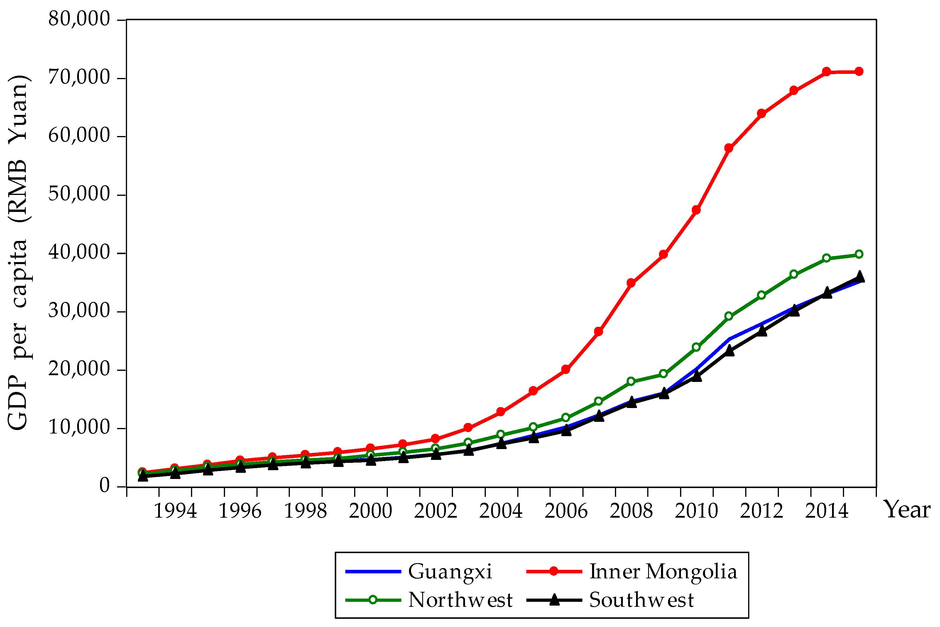
Figure 3.
Krugman index of five southwestern provinces.
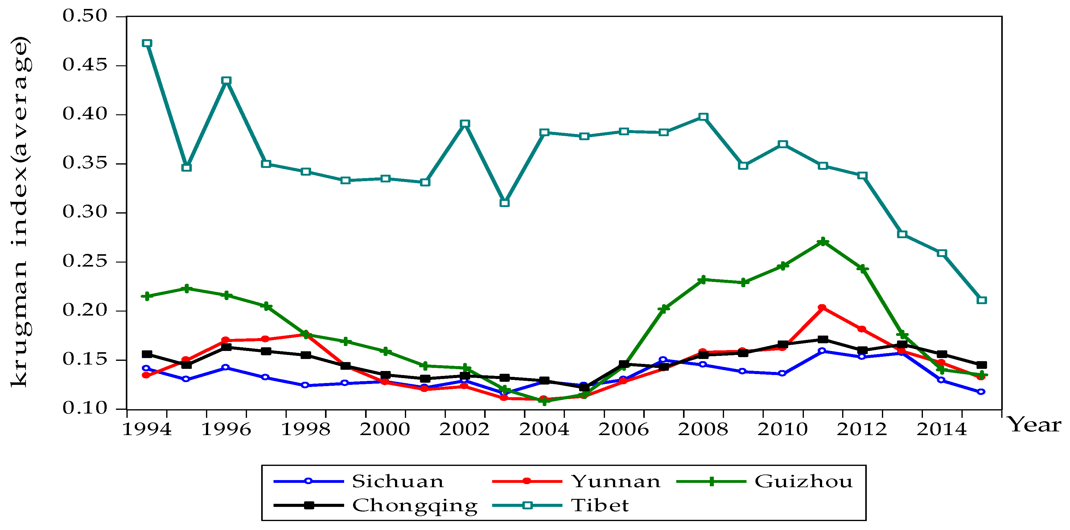
Figure 4.
Krugman index of five northwestern provinces.
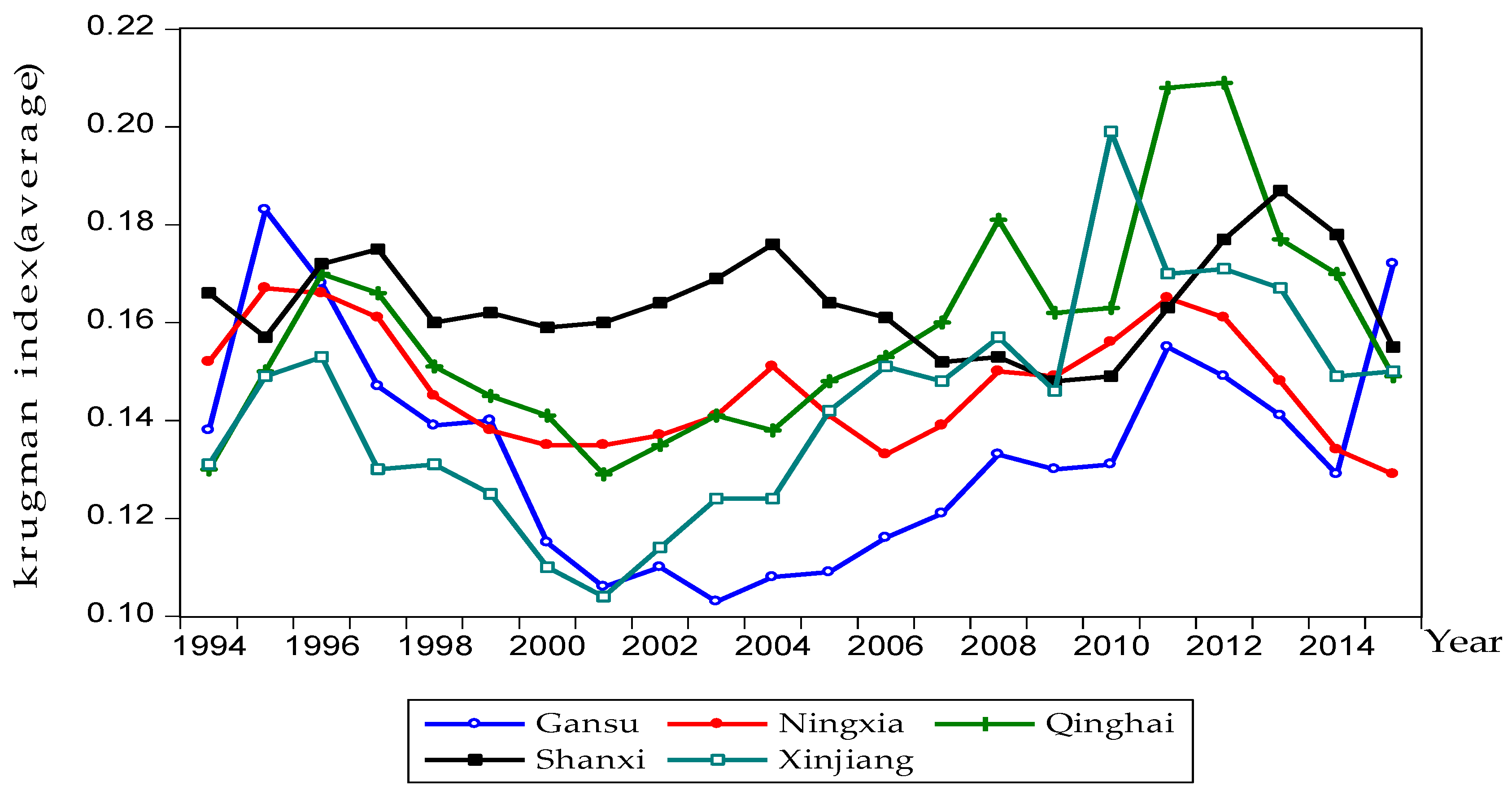
Figure 5.
Krugman index comparison of southwestern, northwestern China, Inner Mongolia and Guangxi.
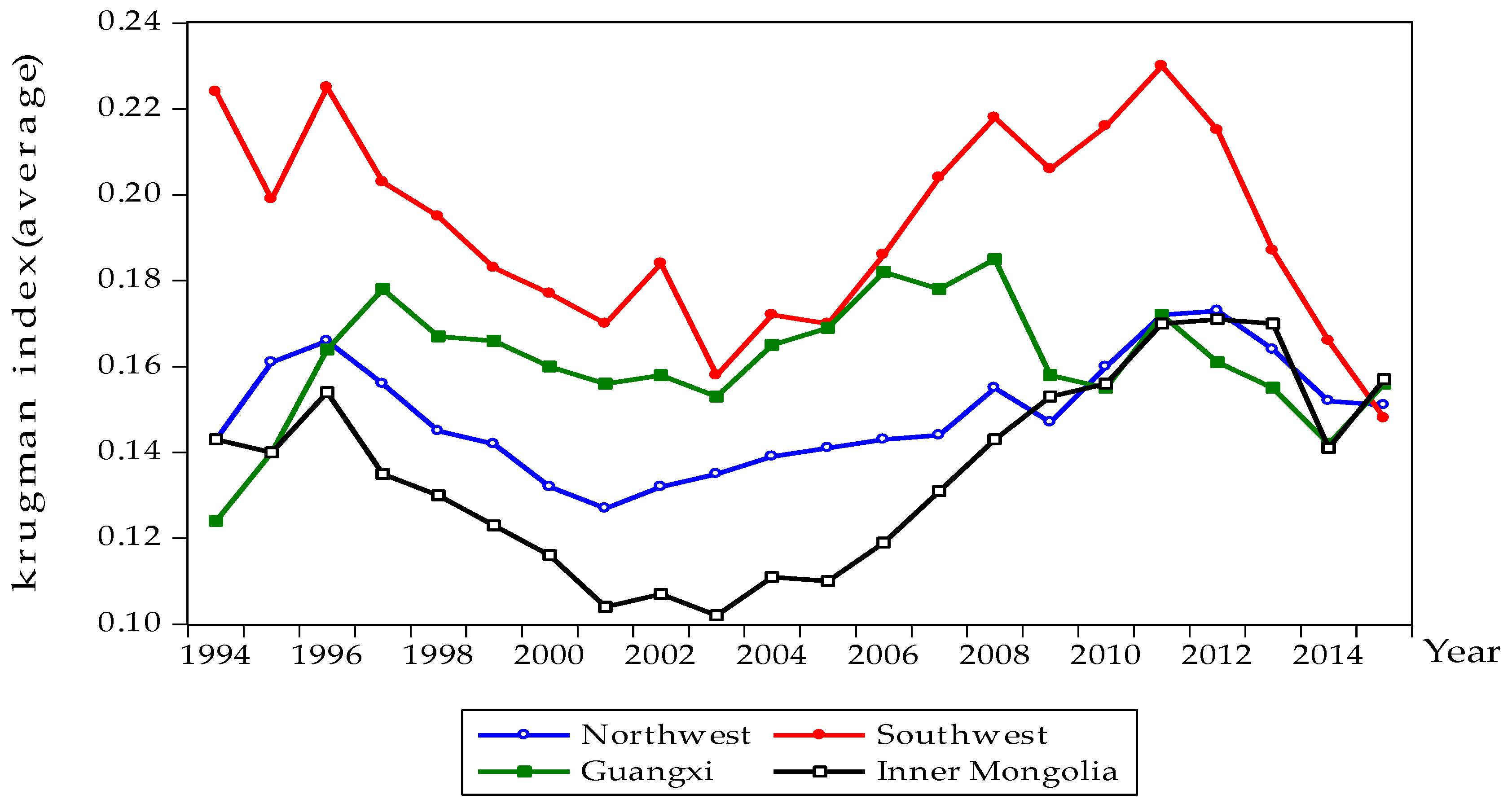
Figure 6.
Moran’s I of human capital from 2003 to 2015.

Figure 7.
Distribution of human capital in western China in 2003.
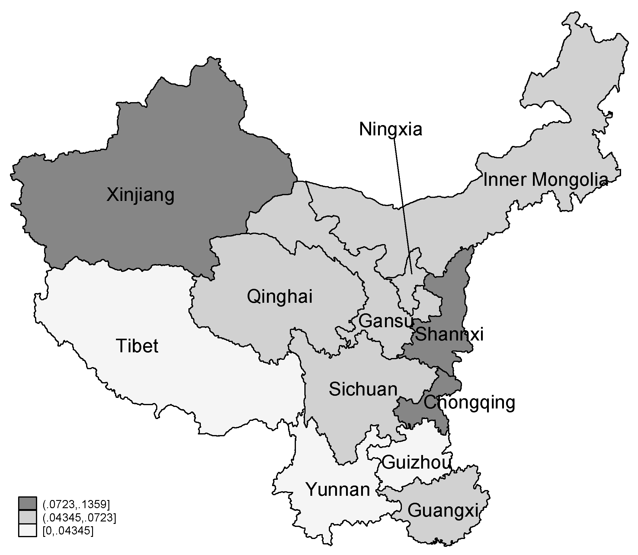
Figure 8.
Distribution of human capital in western China in 2015.


Table 1.
Factors influencing regional economic difference.
| Natural logarithm of GDP per capita at the end of each year | Factor | Indicator | Symbol | Explanation | Data Source | Cite Source |
| Capital Matrix | Total capital formation | TCF | Net amount of fixed assets and inventories obtained within a certain period of time minus disposal | Download the annual data of the province from the National Bureau of Statistics (available at http: Jan Data stats. Gov. Cn Easyquery. htmCnco C01) | Xu, Fei et al. (2011) [36] | |
| Fixed assets investment | FAI | Non-monetary assets | Download the annual data of the province from the National Bureau of Statistics (available at http: Jan Data stats. Gov. Cn Easyquery. htmCnco C01) | Kong, Lingshuai (2013) [33] | ||
| Government Expenditure | Financial expenditure | FE | Investment expenditure of the Government | Download the annual data of the province from the National Bureau of Statistics (available at http: Jan Data stats. Gov. Cn Easyquery. htmCnco C01) | Li, Shuhong (2011) [32] | |
| External Environment | Foreign direct investment | FDI | Regional attraction of foreign investment | Download the annual data of the province from the National Bureau of Statistics (available at http: Jan Data stats. Gov. Cn Easyquery. htmCnco C01) | Jean-Claude Berthelemy, etc. (2000) [26] | |
| Infrastructure Matrix | Railway line length | RLL | Reflecting traffic conditions | Download the annual data of the province from the National Bureau of Statistics (available at http: Jan Data stats. Gov. Cn Easyquery. htmCnco C01) | Wang, Fengxue (2012) [37] | |
| Ordinary higher school | OHS | The construction of education | Download the annual data of the province from the National Bureau of Statistics (available at http: Jan Data stats. Gov. Cn Easyquery. htmCnco C01) | New factor | ||
| Medical institutions | MI | Health care | Download the annual data of the province from the National Bureau of Statistics (available at http: Jan Data stats. Gov. Cn Easyquery. htmCnco C01) | New factor | ||
| Knowledge Innovation Matrix | Human capital | HC | Reflecting education | Belton Fleisher et al. (2010) [27] | ||
| Patent authorization | PA | The representation of innovative ability | Download the annual data of the province from the National Bureau of Statistics (available at http: Jan Data stats. Gov. Cn Easyquery. htmCnco C01) | Wu, You (2012) [31] | ||
| Space Lag Variable | W* Human capital | WHC | Reflecting the spatial spillover effect | The weighted matrix calculated by the adjacency criterion * human capital: W*HC | Riccardo Crescenzi et al. (2014) [40,41] | |
| W* Foreign direct investment | WFDI | Reflecting the spatial spillover effect | Weight matrix calculated by Adjacency criterion * Patent Application authorization Amount: W*FDI | Riccardo Crescenzi et al.. (2014) [40,41] | ||
| Control Variables | Degree of industrial isomorphism | Krugman | Measuring the overall difference of industrial structure between regions | Zhao, Ye et al. (2016) [42] | ||
| Population density | PD | Indicators that indicate the intensity of the population everywhere | Total population of area at the end of the year/Total land area of area | Riccardo Crescenzi et al. (2014) [40,41] | ||
| West development dummy variables | DWEST | Major strategic policies in the western region | 0,1 dummy variables It is 0 before 2000, it is 1 after 2000 | Liu, Shenglong(2009) [43] |
Table 2.
Demographics description of variables obs = 264.
| Variable | Mean | Standard Deviation | Minimum | Maximum |
|---|---|---|---|---|
| Y | 9.20928 | 0.9166225 | 7.33 | 11.17 |
| TCF | 2714.305 | 3556.76 | 23.07 | 15,728.14 |
| FAI | 3129.583 | 4598.551 | 21.17 | 25,525.9 |
| FE | 1071.08 | 1363.291 | 19.38 | 7497.51 |
| FDI | 11,003.27 | 15,249.63 | 93 | 88,409 |
| RLL | 0.2475379 | 0.1881398 | 0 | 1.21 |
| OHS | 35.30682 | 24.55228 | 3 | 109 |
| MI | 13,431.57 | 14,263.64 | 476 | 81,070 |
| HC | 0.0832909 | 0.062462 | 0.0094 | 0.2913 |
| PA | 3717.205 | 8120.965 | 2 | 64,953 |
| WHC | 0.3401163 | 0.2635785 | 0.0225 | 1.1797 |
| WFDI | 46,997.64 | 47,905.25 | 989 | 242,503 |
| Krugman | 0.1670833 | 0.0630569 | 0.102 | 0.473 |
| PD | 116.382 | 102.013 | 1.91 | 364.56 |
| DWEST | 0.7272727 | 0.4462077 | 0 | 1 |
| LNFE | 6.141705 | 1.39288 | 2.96 | 8.92 |
| LNTCF | 7.044091 | 1.434999 | 3.14 | 9.66 |
| LNFAI | 7.010985 | 1.547257 | 3.05 | 10.15 |
Table 3.
Moran’s I.
| Year | Variables | I | sd(I) | z | p-Value * |
|---|---|---|---|---|---|
| 1994 | HC | 0.187 | 0.156 | 1.783 | 0.075 |
| 1995 | HC | 0.160 | 0.156 | 1.605 | 0.108 |
| 1996 | HC | 0.152 | 0.152 | 1.603 | 0.109 |
| 1997 | HC | 0.145 | 0.150 | 1.567 | 0.117 |
| 1998 | HC | 0.119 | 0.145 | 1.453 | 0.146 |
| 1999 | HC | 0.112 | 0.140 | 1.453 | 0.146 |
| 2000 | HC | 0.110 | 0.142 | 1.418 | 0.156 |
| 2001 | HC | 0.156 | 0.147 | 1.679 | 0.093 |
| 2002 | HC | 0.168 | 0.142 | 1.816 | 0.069 |
| 2003 | HC | 0.208 | 0.138 | 2.157 | 0.031 |
| 2004 | HC | 0.223 | 0.136 | 2.308 | 0.021 |
| 2005 | HC | 0.214 | 0.135 | 2.252 | 0.024 |
| 2006 | HC | 0.219 | 0.139 | 2.229 | 0.026 |
| 2007 | HC | 0.234 | 0.143 | 2.270 | 0.023 |
| 2008 | HC | 0.257 | 0.144 | 2.424 | 0.015 |
| 2009 | HC | 0.276 | 0.145 | 2.540 | 0.011 |
| 2010 | HC | 0.267 | 0.147 | 2.425 | 0.015 |
| 2011 | HC | 0.284 | 0.150 | 2.489 | 0.013 |
| 2012 | HC | 0.301 | 0.152 | 2.584 | 0.010 |
| 2013 | HC | 0.316 | 0.151 | 2.692 | 0.007 |
| 2014 | HC | 0.330 | 0.153 | 2.750 | 0.006 |
| 2015 | HC | 0.341 | 0.155 | 2.791 | 0.005 |
* Two-tail test.
Table 4.
Compared FGLS(Feasible generalized least squar) analysis of the proposed regression model.
| Variable | (1) | (2) |
|---|---|---|
| LNTCF | 0.318 *** | 0.368 *** |
| (12.03) | (13.80) | |
| LNFAI | 0.245 *** | 0.174 *** |
| (8.36) | (6.02) | |
| LNFE | 0.0848 *** | 0.0830 *** |
| (3.32) | (3.48) | |
| FDI | 0.000000750 | 0.000000640 |
| (1.07) | (0.88) | |
| RLL | 0.120 | 0.255 *** |
| (1.83) | (3.71) | |
| OHS | −0.000986 | −0.00177** |
| (−1.67) | (−3.12) | |
| MI | −0.00000129 ** | −0.00000107 ** |
| (−3.21) | (−2.85) | |
| HC | 1.583 *** | 1.301 *** |
| (4.97) | (4.10) | |
| PA | 0.00000341 *** | 0.00000137 |
| (3.89) | (1.52) | |
| WHC | 0.141 ** | |
| (3.03) | ||
| WFDI | 0.000000953 *** | |
| (4.42) | ||
| Krugman | 1.033 *** | 1.037 *** |
| (7.34) | (9.25) | |
| PD | −0.00391 *** | −0.00321 *** |
| (−6.45) | (−5.31) | |
| DWEST | 0.0201 | 0.0310 |
| (1.13) | (1.82) | |
| province2 | −1.265 *** | −1.175 *** |
| (−5.93) | (−5.52) | |
| province3 | −0.947 *** | −0.830 *** |
| (−6.51) | (−5.59) | |
| province4 | −0.997 *** | −0.993 *** |
| (−6.88) | (−6.76) | |
| province5 | −1.192 *** | −1.062 *** |
| (−5.06) | (−4.51) | |
| province6 | −0.247 | −0.139 |
| (−1.25) | (−0.70) | |
| province7 | −0.507 * | −0.367 |
| (−2.11) | (−1.53) | |
| province8 | −1.406 *** | −1.315 *** |
| (−8.87) | (−8.28) | |
| province9 | −1.040 *** | −0.966 *** |
| (−6.56) | (−6.04) | |
| Province 10 | −1.194 *** | −0.974 *** |
| (−5.06) | (−4.13) | |
| Province 11 | −0.408 | −0.262 |
| (−1.43) | (−0.92) | |
| Province 12 | −1.339 *** | −1.224 *** |
| (−7.25) | (−6.56) | |
| _cons | 5.745 *** | 5.638 *** |
| (22.37) | (22.01) | |
| N | 264 | 264 |
Note: t statistics in parentheses; * p < 0.05, ** p < 0.01, *** p < 0.001; Prob>chi2 = 0.0000; (1) refers to a FGLS model without the consideration of space factors; (2) refers to a FGLS model with the consideration of space factors.
Table 5.
Robust test results of filter variable method. Cross-sectional time-series FGLS regression.
Table 5.
Robust test results of filter variable method. Cross-sectional time-series FGLS regression.
| Variable | (1) | (2) |
|---|---|---|
| LNTCF | 0.310 *** | 0.336 *** |
| (11.95) | (12.76) | |
| LNFAI | 0.257 *** | 0.216 *** |
| (9.20) | (7.94) | |
| LNFE | 0.0885 *** | 0.0930 *** |
| (3.57) | (3.81) | |
| FDI | 0.000000380 | 0.000000130 |
| (0.58) | (0.18) | |
| MI | −0.00000142 *** | −0.00000122 ** |
| (−3.59) | (−3.04) | |
| HC | 1.396 *** | 0.972 *** |
| (4.73) | (3.32) | |
| PA | 0.00000343 *** | 0.00000180 |
| (3.95) | (1.83) | |
| WHC | 0.0986 * | |
| (2.00) | ||
| WFDI | 0.000000762 *** | |
| (3.40) | ||
| Krugman | 1.003 *** | 1.028 *** |
| (7.10) | (8.58) | |
| PD | −0.00378 *** | −0.00300 *** |
| (−6.02) | (−4.72) | |
| DWEST | 0.00936 | 0.0105 |
| (0.57) | (0.64) | |
| Province 2 | −1.211 *** | −1.055 *** |
| (−5.50) | (−4.76) | |
| Province 3 | −0.924 *** | −0.793 *** |
| (−6.17) | (−5.15) | |
| Province 4 | −0.979 *** | −0.946 *** |
| (−6.55) | (−6.21) | |
| Province 5 | −1.077 *** | −0.834 *** |
| (−4.52) | (−3.46) | |
| Province 6 | −0.191 | −0.0274 |
| (−0.94) | (−0.13) | |
| Province 7 | −0.436 | −0.229 |
| (−1.76) | (−0.91) | |
| Province 8 | −1.399 *** | −1.292 *** |
| (−8.66) | (−7.87) | |
| Province 9 | −1.015 *** | −0.905 *** |
| (−6.25) | (−5.47) | |
| Province 10 | −1.130*** | −0.860 *** |
| (−4.65) | (−3.49) | |
| Province 11 | −0.338 | −0.140 |
| (−1.15) | (−0.47) | |
| Province 12 | −1.317 *** | −1.177 *** |
| (−6.89) | (−6.04) | |
| _cons | 5.656 *** | 5.459 *** |
| (21.41) | (20.65) | |
| N | 264 | 264 |
Note: t statistics in parentheses; * p < 0.05, ** p < 0.01, *** p < 0.001; (1) refers to a FGLS model with space factors, (2) refers to a FGLS model without space factors.
Table 6.
Robustness Test Results of SLM and SEM.
| Variable | SLM | SEM |
|---|---|---|
| Wy | 0.219 *** | |
| (3.98) | ||
| LNTCF | 0.218 *** | 0.238 *** |
| (3.41) | (3.73) | |
| LNFAI | 0.212 ** | 0.283 *** |
| (2.86) | (3.74) | |
| LNFE | 0.0605 | 0.148 ** |
| (1.20) | (2.68) | |
| FDI | 0.000000177 | 0.00000191 |
| (0.08) | (0.92) | |
| HC | 0.762 | 0.920 |
| (1.49) | (1.66) | |
| RLL | 0.0827 | 0.150 |
| (0.57) | (1.05) | |
| OHS | −0.000433 | −0.000533 |
| (−0.30) | (−0.33) | |
| MI | −0.00000114 | −0.000000211 |
| (−0.81) | (−0.13) | |
| PA | 0.00000162 | 0.00000550 |
| (0.46) | (1.52) | |
| PD | −0.00346 | −0.00507 ** |
| (−1.90) | (−2.64) | |
| DWEST | 0.0162 | 0.00852 |
| (0.55) | (0.21) | |
| Krugman | 0.855 ** | 0.837 ** |
| (2.79) | (2.64) | |
| Province 2 | −1.486 ** | −3.262 ** |
| (−2.62) | (−3.17) | |
| Province 3 | −0.705 * | −0.396 |
| (−2.49) | (−1.06) | |
| Province 4 | −1.003 *** | −1.645 *** |
| (−3.77) | (−4.86) | |
| Province 5 | −1.068 | −1.529 * |
| (−1.78) | (−2.53) | |
| Province 6 | −0.345 | −0.473 |
| (−0.73) | (−1.00) | |
| Province 7 | −0.708 | −1.538 |
| (−1.15) | (−1.94) | |
| Province 8 | −1.618 *** | −3.905 *** |
| (−3.88) | (−3.48) | |
| Province 9 | −1.101 ** | −2.307 *** |
| (−3.24) | (−3.52) | |
| Province 10 | −1.091 | −1.562 * |
| (−1.80) | (−2.53) | |
| Province 11 | −0.645 | −1.342 |
| (−1.04) | (−1.76) | |
| Province 12 | −1.281 ** | −2.119 *** |
| (−2.96) | (−3.96) | |
| _cons | 4.477 *** | 4.702 *** |
| (6.46) | (6.11) | |
| Rho | ||
| _cons | 0.0123 | |
| (1.66) | ||
| sigma | ||
| _cons | 0.116 *** | 0.119 *** |
| (22.98) | (22.98) | |
| lambda | ||
| _cons | 0.0854 ** | |
| (2.76) | ||
| N | 264 | 264 |
Note: t statistics in parentheses; * p < 0.05, ** p < 0.01, *** p < 0.001.
© 2017 by the authors. Licensee MDPI, Basel, Switzerland. This article is an open access article distributed under the terms and conditions of the Creative Commons Attribution (CC BY) license (http://creativecommons.org/licenses/by/4.0/).
Share and Cite
MDPI and ACS Style
Zhang, J.; Liu, Q.; Wang, C.; Li, H. Spatial–Temporal Modeling for Regional Economic Development: A Quantitative Analysis with Panel Data from Western China. Sustainability 2017, 9, 1955. https://doi.org/10.3390/su9111955
AMA Style
Zhang J, Liu Q, Wang C, Li H. Spatial–Temporal Modeling for Regional Economic Development: A Quantitative Analysis with Panel Data from Western China. Sustainability. 2017; 9(11):1955. https://doi.org/10.3390/su9111955
Chicago/Turabian StyleZhang, Jingxiao, Qiaoling Liu, Chao Wang, and Hui Li. 2017. "Spatial–Temporal Modeling for Regional Economic Development: A Quantitative Analysis with Panel Data from Western China" Sustainability 9, no. 11: 1955. https://doi.org/10.3390/su9111955
Note that from the first issue of 2016, this journal uses article numbers instead of page numbers. See further details here.