Energy Savings from Optimised In-Field Route Planning for Agricultural Machinery
by
 , and
, and
Efthymios Rodias
1,*, 
Remigio Berruto
1,
Patrizia Busato
1,
Dionysis Bochtis
2,3,
Claus Grøn Sørensen
3 and
and
Kun Zhou
3 1
Department of Agriculture, Forestry and Food Science (DISAFA), Faculty of Agriculture, University of Turin, Largo Braccini 2, 10095 Grugliasco, Italy
2
Institute for Bio-economy and Agri-Technology (IBO), Centre for Research & Technology—Hellas (CERTH), 57001 Thessaloniki, Greece
3
Department of Engineering, Faculty Science and Technology, Aarhus University, 8000 Aarhus, Denmark
*
Author to whom correspondence should be addressed.
Sustainability 2017, 9(11), 1956; https://doi.org/10.3390/su9111956
Submission received: 31 July 2017
/
Revised: 12 October 2017
/
Accepted: 22 October 2017
/
Published: 27 October 2017
(This article belongs to the Special Issue Precision Agriculture Technologies for a Sustainable Future: Current Trends and Perspectives)
Abstract
:Various types of sensors technologies, such as machine vision and global positioning system (GPS) have been implemented in navigation of agricultural vehicles. Automated navigation systems have proved the potential for the execution of optimised route plans for field area coverage. This paper presents an assessment of the reduction of the energy requirements derived from the implementation of optimised field area coverage planning. The assessment regards the analysis of the energy requirements and the comparison between the non-optimised and optimised plans for field area coverage in the whole sequence of operations required in two different cropping systems: Miscanthus and Switchgrass production. An algorithmic approach for the simulation of the executed field operations by following both non-optimised and optimised field-work patterns was developed. As a result, the corresponding time requirements were estimated as the basis of the subsequent energy cost analysis. Based on the results, the optimised routes reduce the fuel energy consumption up to 8%, the embodied energy consumption up to 7%, and the total energy consumption from 3% up to 8%.
1. Introduction
The satellite system GNSS (Global Navigation Satellite System) is used to pinpoint the geographic location of a user’s receiver anywhere in the world. The main GNSS systems that are currently in operation are the Global Positioning System (GPS), the Global Orbiting Navigation Satellite System (GLONASS) and the Galileo. Each of these systems employs a group of orbiting satellites working in connection with a network of ground stations. In modern agriculture, automation systems are part of any kind of agricultural machinery and agricultural vehicles (tractors and self-propelled machines). Various types of technologies, such as machine vision and satellite systems as GPS, have been implemented in navigation of agricultural vehicles [1,2,3,4,5,6]. The fully automated auto-steering systems are capable of driving the agricultural vehicle either in a straight or in a curved line over the field area with a lateral accuracy of a few centimetres when making use of highly accurate real-time kinematic (RTK) GPS receivers. Auto-steering systems based navigation can apply in any field operation, including planting, cultivating and harvest [7]. The position information from RTK GPS systems can be used not only for guidance but also for other applications such as seed mapping, controlled traffic, and controlled tillage [8].
Automated navigation systems have also provided the potential for the execution of optimised route plans for field area coverage. In the non-optimised practice of covering a field area, the route of an agricultural vehicle consists of a series of back-and-forth repetitions that follow a standard motif, such as, for example, to always enter the adjacent field-work track of the one that has been worked. On the other hand, optimised field area coverage provides routes that cannot be executed without the implementation of navigation-aiding systems. Recently, a number of route planning methods for field area coverage have been developed [9,10,11,12,13,14,15,16,17]. Bochtis and Soerensen showed the potential of the vehicle routing problem (VRP) application and agricultural vehicles area coverage planning [12]. The implementation of the approach in field operations executed by conventional agricultural machines equipped with auto-steering systems has reduced the total non-working travelled distance up to 50%, as it has been experimentally shown [18]. This optimised new type of field-work patterns, called B-patterns, is defined as: “algorithmically-computed sequences of field-work tracks completely covering an area and that do not follow any pre-determined standard motif, but in contrast, are a result of an optimisation process under one or more selected criteria” [19]. An example of the optimisation of route planning compared to the non-optimised for two operating widths (6 m and 12 m) is presented in Figure 1.
The benefits from B-patterns are significant reductions in non-working distance and increases in the area capacity compared to different types of non-optimised field-work patterns. The optimal route planning may focus on one or more optimisation criterion such as, total or non-working distance, total operational time, and so forth [20,21], and it is directly connected with operating width and the minimum turning radios of the agricultural vehicle. The benefits from optimal route planning are directly correlated to fuel consumption and field machinery use. As a direct consequence, there is an energy cost reduction in the field operations when implementing optimised field-work patterns. The objective of this paper is to provide an assessment of the reduction of the energy requirements derived from the implementation of B-patterns. The assessment regards the analysis of the energy requirements and the comparison between the non-optimised and optimised plans for field area coverage in the whole sequence of operations required in a cropping system. Two cropping systems have been selected, namely, Miscanthus (Miscanthus × giganteus) production and Switchgrass (Panicum virgatum) production.
The structure of the present work is as follows: initially, a presentation of the methodology in terms of the main input parameters and the design of the assessment approach is introduced. This is followed by the results section, where two case scenarios are provided together with the energy cost analysis of the presented case studies. The paper wraps up with the discussion of the results.
2. Materials and Methods
The assessment is based on the savings in time requirements, including both working time and non-working time from the implementation of the optimised field-work-patterns, which result in savings in energy consumption compared with the non-optimised field-work patterns. This assessment does not include operations with coupled machines, where a primary unit has to be supported by a secondary unit as a service unit (for example, the harvesting tractor-wagon set). In the present study, for the harvesting operation, it is considered that the harvester has an on-board wagon to deliver the harvested material. The assessment of this study is based on combinations derived from the consideration of five field shapes, one type of non-optimised field-work pattern (AB-pattern: from A track line to B track line, and so on), two cropping systems case studies, and various combinations of implement operating widths and minimum turning radii.
For the abovementioned assessment the following assumptions have been considered:
- The covering of the headland area has been excluded from the comparison, and only the covering of the main field area has been considered.
- All the operations are executed continuously without any load capacity restriction.
- During the turnings the fuel consumption is considered to be the same as the one during the operation.
- The energy consumption for the material transportation is not considered in the comparison.
- The energy consumption for the machinery transportation from farm to field is not considered in the comparison.
- It has been considered that the field entrance can be anywhere in the field boundary.
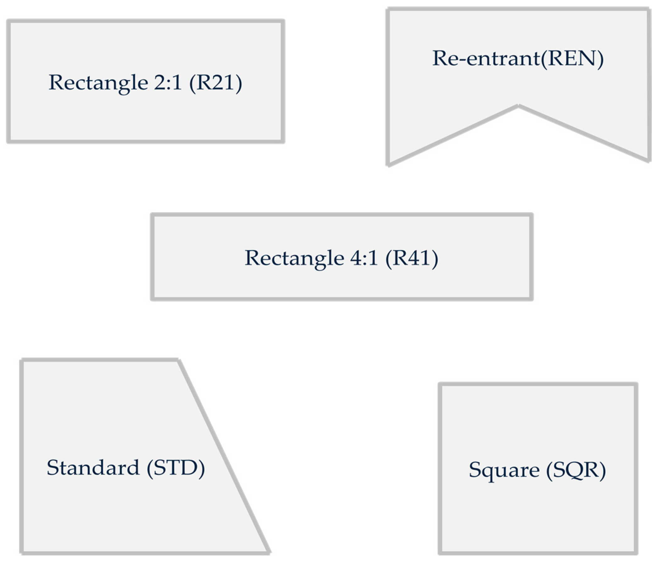
2.1. Field Shapes
2.2. Cropping Systems
This assessment was run in two energy crops as case studies, namely, CS1 for Miscanthus crop and CS2 for Switchgrass crop, in order to compare the results and evaluate the methodology under different crop production requirements. Both crops were evaluated for the basic in-field operations that are normally applied.
Miscanthus cultivation does not require any special soil management [23,24]. Thus, a light ploughing up to 20 cm in depth and a disk-harrowing were considered as the basic soil preparation operations. Afterwards and before the establishment of the crop, it is important to carry out weed control thoroughly to minimize weed competitiveness. After that, there is no need for weed control since the crop can protect itself from the weeds. Here, a single herbicide application has been considered as a pre-planting weed control. Given that Miscanthus is planted by rhizomes, a planter similar to the potato seed planter can be adopted for the planting operation. Irrigation should be applied in parallel with rainfall but it is beyond the scope of the current study. Miscanthus does not have high nutrient requirements since the crop itself can absorb most of the required nutrients from the soil. However, it has been reported that the addition of 50 kg N, 21 kg P2O5, and 45 kg K2O per ha per year are sufficient to support adequate yields [25]. This fertilizers’ allocation has been implemented in this study. Harvesting of the crop usually occurs every year, starting from the second year. It is usually carried out by using conventional forage harvesters for cutting and chopping the biomass.
Regarding Switchgrass, seedbeds are normally prepared by traditional ploughing and secondary cultivation processes. Here, ploughing and disk harrowing were considered for the soil preparation. During the first growth, it is crucial for the seedbed to be thoroughly weed controlled given that the crop is not competitive during the first establishment phase [26]. For this, a pre-seeding herbicide control was considered. Switchgrass is established by seed. As in the case of Miscanthus, apart from rainfall, irrigation is important but is not included in the presented study’s scope. Switchgrass can provide high yields even under limited fertilization of 75 kg N·ha−1 [27]. In the establishment year, no nitrogen should be applied, as it can promote weed growth leading to competition against the new plants. Phosphorus and potassium should be applied only if soil availability is low. In the following years, the application of nutrients should be at a level that anticipates rising productivity [23]. Switchgrass’s growth is slow in the first year and there is a negative competition with weeds [23]. For this reason, Switchgrass requires weed control both before the establishment and for the next two years. Regarding harvesting, there is no technical reason for the crop not to be cut and harvested by conventional grass harvesting machinery [26]. Before the forage harvester operates, a mower is considered in order to allow to the mowed plants to have adequate time to dry during winter [26].
2.3. Machinery Systems
Based on the operational requirements for the execution of each of the operations included in the abovementioned cropping systems, three different sizes of tractors varying in machine power, weight, productivity, and manoeuvrability (minimum turning radius) were used. More specifically, after extensive research on technical machinery features of different commercial models of tractors, a large-size tractor unit with a 6 m minimum turning radius, a medium-size tractor unit with a 4.5 m minimum turning radius, and a small-size tractor unit with a 3 m minimum turning radius, were selected as representative for the presented assessment. Variable operating widths were considered for the execution of the field operations in the two case studies. In Table 1 the combinations of operating width and turning radius for each executed field operation of the two case studies are presented. The considered combinations were symmetric excluding those that regard (i) small units connected to large operating widths, given that a small unit cannot provide the required power for a large operating width, and (ii) large units combined with very small operating widths. It is worth noting that in the case of ploughing, a modified formulation of the optimisation problem of the one presented in [18] has been considered, that takes into account the operational restrictions of ploughing operation. In particular, the operational restriction derived from the requirements for an even field surface generation regards the turning over of the mounted mouldboards in the reversible plough each time the working direction changes.
2.4. Energy Inputs
The energy inputs that directly or indirectly connected with the agricultural machinery use are shown in Table 2. The diesel energy coefficient that corresponds to the chemical energy of diesel is equal to 41.2 MJ·L−1 [28]. This coefficient is recommended for the United Kingdom and has been adopted for Europe because of the shorter distance that crude oil is transported from the Middle East. It includes crude oil energy content, production energy consumption, shipping energy consumption, and refining/distribution energy consumption. For the estimation of fuels energy cost, the diesel energy coefficient, the operational capacity extracted from the time requirements, the tractor power and the Equation (1) from American Society of Agricultural and Biological Engineers (ASABE) standards for fuels consumption estimation (in L·(kW·h)−1 were taken into account.
where X is the ratio of equivalent power take-off (PTO) power required by an operation to the maximum available power from the PTO [29,30]. Here, X is adopted to be equal to 0.55 for all types of tractors.
2.5. The Assessment Model
The assessment model is presented in Figure 3. The process is as follows: generation of the non-optimised field-work pattern; generation of the optimised field-work pattern; simulation of the operations following the non-optimised field-work pattern; simulation of the operations following the optimised field-work pattern, and; comparison of their results.
Firstly, the estimation of the headland width and the corresponding number of headland passes was taken into account based on the implement’s operating width, the turning radius and the unit’s dimensions. The geometrical representation of the fields was created given the artificial coordinates of the field boundary and the number of headland passes. As a result, the coordinates of the field-work tracks were generated. In a second phase, for the estimation of the paths that connect each possible pair of tracks, the same path planning procedure was followed in order to produce the energy consumption table of the optimisation problem. The problem was solved by applying the Clarke and Wright savings algorithm and, consequently, the optimised field-work pattern was generated [33]. The tracks sequence of the non-optimised AB field coverage was created given its geometrical field representation and mathematical description. Then the simulation of both non-optimised and optimised field-work patterns was implemented.
3. Results and Discussion
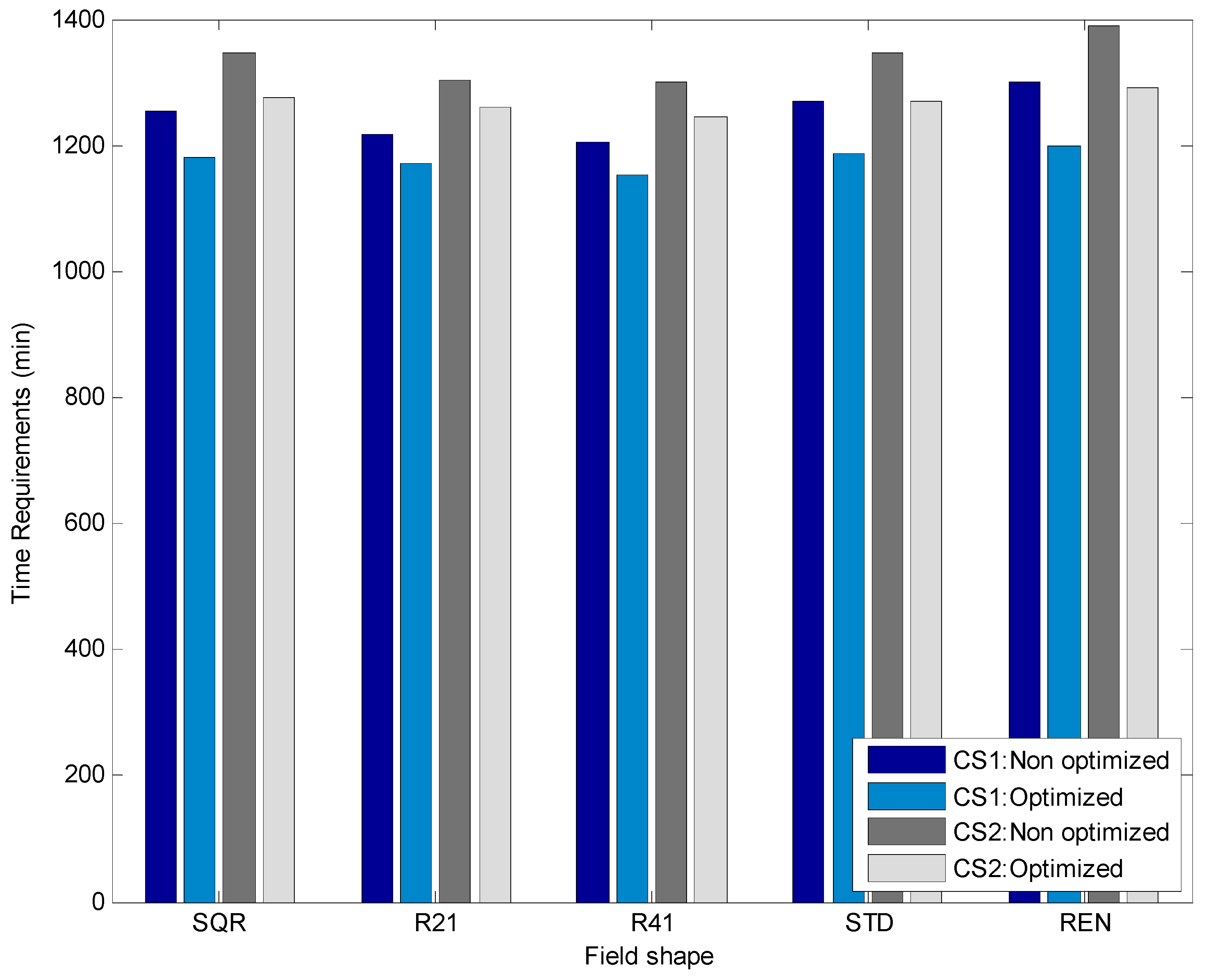
3.1. Time Requirements
The current study regards the effect of the field shape on the execution time of each operation of the two case studies, including the effective and the non-working time. Both the non-optimised and the optimised field pattern scenarios where assessed and they are presented in the Table 3 regarding the considered field operations of the two case studies. In this table the time requirements in minutes are provided in order to demonstrate the time savings per operation. In Figure 4, the total time requirements for the different field shapes of the two case studies, including both non optimised and optimised field route planning, are shown.
3.2. Energy Cost Analysis
Given the abovementioned time requirements results per operation, the field area capacity (ha·h−1) can be obtained for each operation of the two case studies. For the energy cost analysis, several studies have been conducted, pointing out the most important energy factors in single- or multiple-crop production systems [23,34,35]. For the estimation of the energy cost of a crop, many energy inputs and other agronomical related inputs are taken into account, such as field machinery and implements inputs (such as fuels and lubricants energy, embodied energy, weights, estimated lives, etc.), operation-related inputs (operating width, turning radius, area capacity, etc.) and agrochemical material-related inputs (such as applied dosages of fertilizers and agrochemicals). In the current study, the energy cost parameters are connected to fuels energy and field machinery embodied energy. The material-related energy consumption is not included in this study, given that this study focuses on energy savings that are directly or indirectly associated with field machinery.
The fuel energy savings (%) when optimised field-work pattern is used instead of the non-optimised for the corresponding field operations of the two case studies for the five different field shapes are presented in Table 4. The energy savings are related to the non-optimised field-work pattern. In Figure 5, the total energy savings (%) by fuels consumption is presented for the different field shapes.
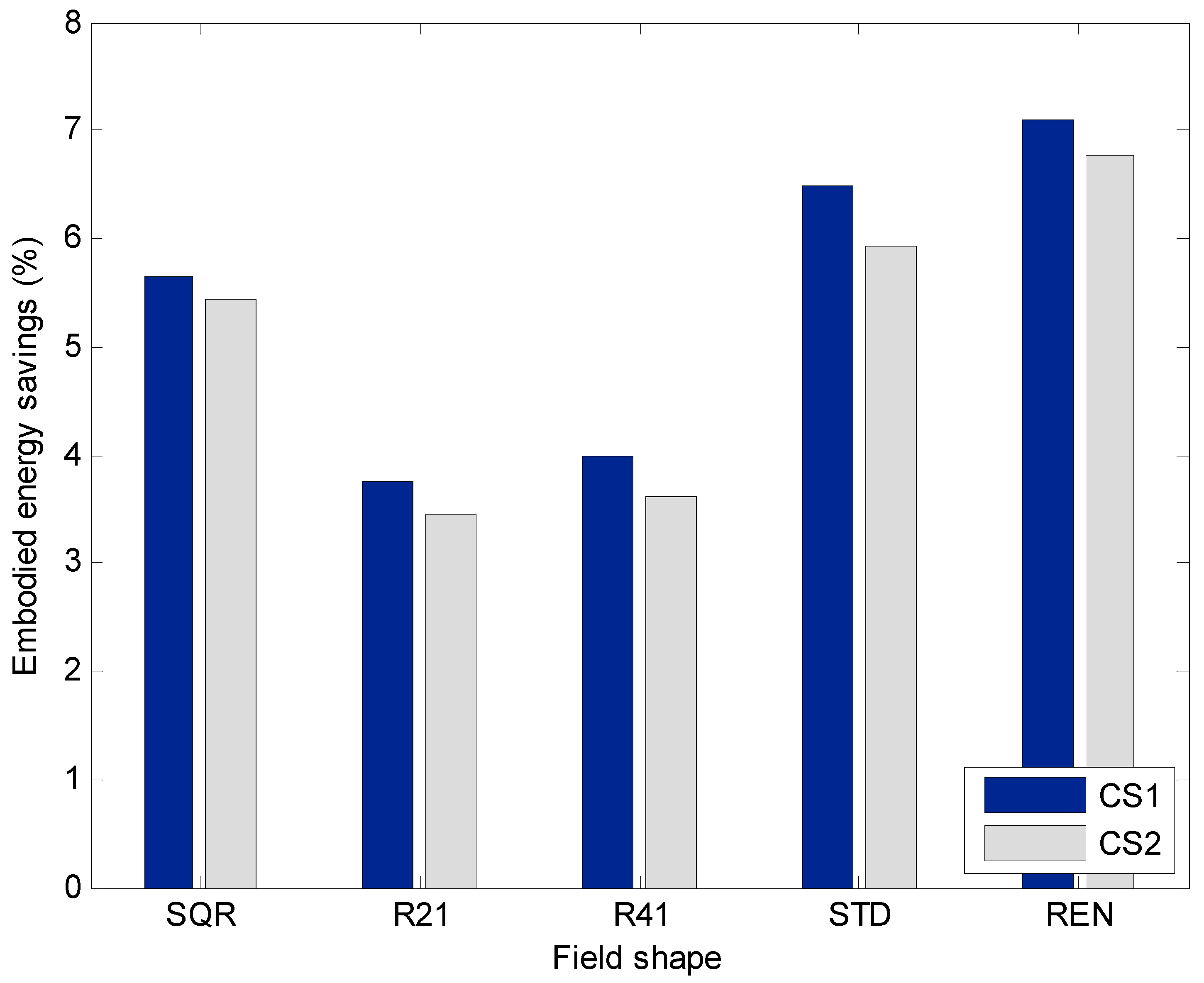
Regarding the second most important energy cost parameter estimation, that is, the field machinery embodied energy, the factors that are included are the operational capacity, the total embodied energy of the tractor and its implement over their whole lifetime (in MJ), their estimated lifetimes, and their weights. Given these, the corresponding energy consumption of both tractor and implement for the total operational time were estimated for both non-optimised and optimised field-work patterns in the five different field shapes. In Table 5, the energy savings (%) from machinery embodied energy by following the optimised field-work pattern in the five different field shapes for both case studies is demonstrated. The energy savings are related to the non-optimised field-work pattern. Also, the energy savings (%) from machinery embodied energy including all the operations per field shape in both case studies are presented in Figure 6.
It should be highlighted that this study focuses only on the most significant energy consumption factors as they have already mentioned above. There are other less significant factors such as lubricant energy cost that contribute much less to the total energy consumption. It should be mentioned, also, that each of these energy inputs contributes under different impact factor to the total energy cost savings results. In Figure 7 the total energy savings (%), including all the field operations by using the optimised field-work pattern in the five field shapes for both case studies, are shown.
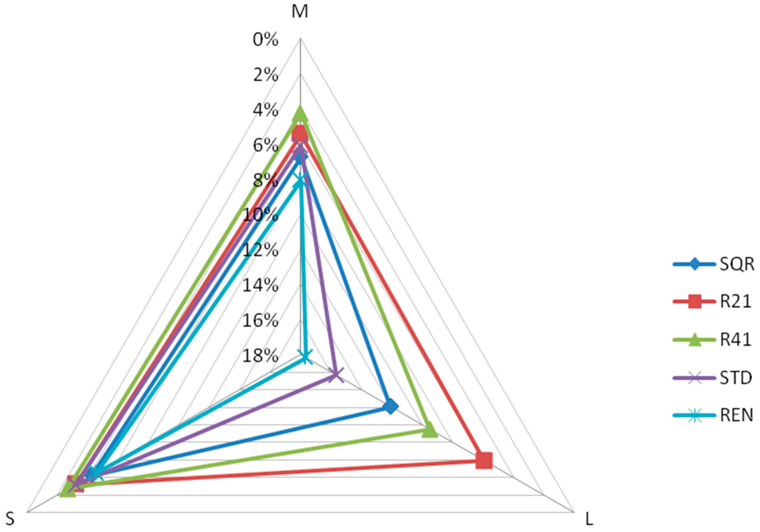
3.3. The Effect of Machinery Size
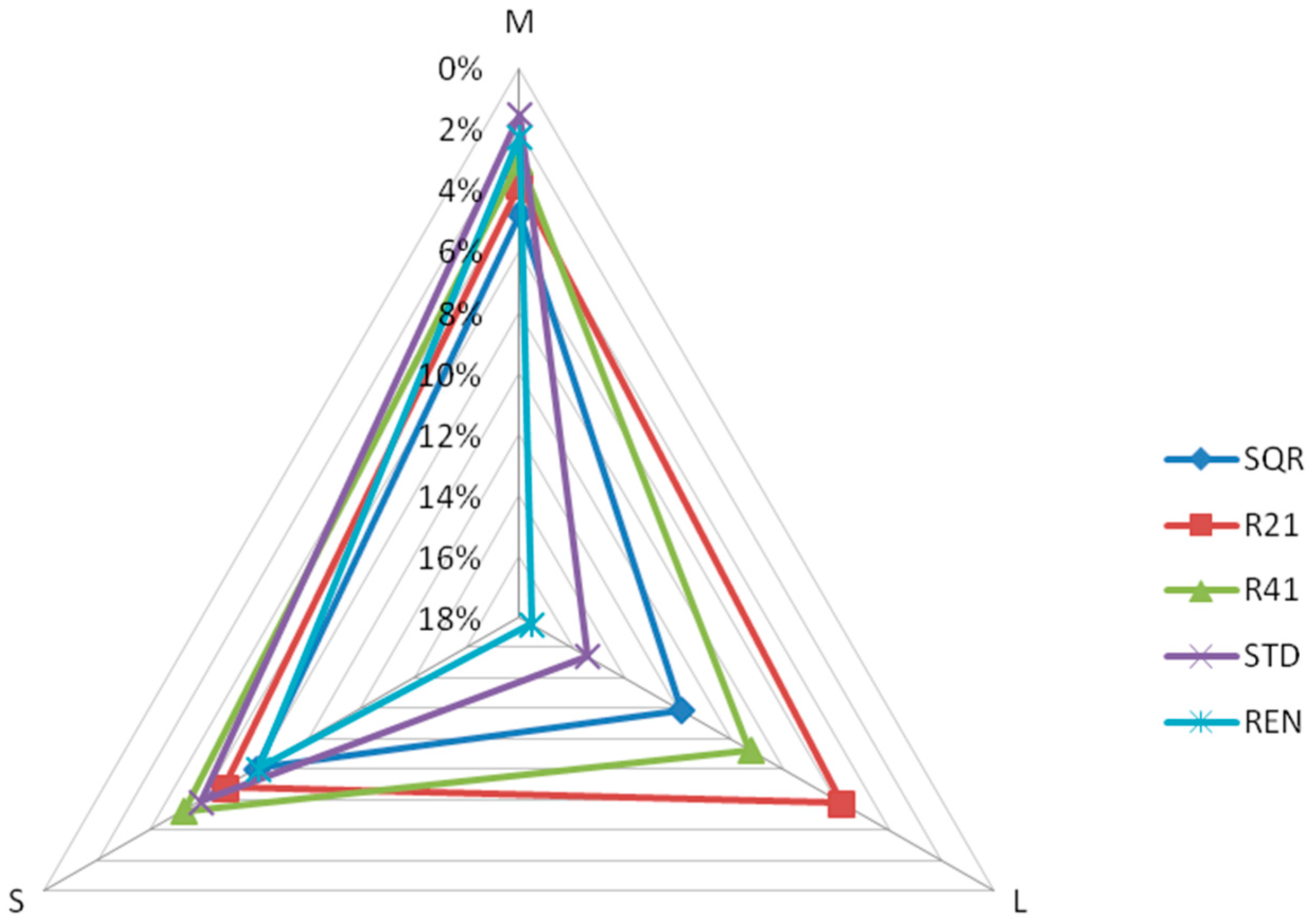
The assessment of the energy cost savings for the two case studies has been based on specific machinery systems in terms of operating width and minimum turning radius. The selection of these machinery systems was based on the optimum combination tractor size and equipment for each specific field operation requirements. However, in real-life cases the implemented machinery systems in various operations are the ones that are available in the farm and in the majority of the cases is not the optimum selection in terms of machinery size. The effect of the different tractor sizes (S: Small-sized tractor (up to 50 kW); M: Medium-sized tractor (up to 120 kW), and; L: Large-sized tractor (up to 180 kW)) on the total energy savings (%) in the optimised scenarios is presented in Figure 8 and Figure 9, for the CS1 and CS2, respectively. The selection of the size of the combination tractor-machinery is directly connected to the minimum turning radius and the operating width that are used in any specific field operation. In cases where the selection of machinery size is not optimum, the energy savings when optimised plan is applied can be up to 18%.
4. Conclusions
An assessment on the energy savings by applying optimised field-work patterns in field machinery operations was presented in this paper. A comparison between the most widely implemented non-optimised field-work pattern (AB-pattern) and an optimised one (B-pattern) was presented under the criterion of time requirements, which is the basis for the subsequent energy cost analysis. The energy cost analysis for both field-work patterns demonstrated a reduction in the operational energy requirements in the range of 3–8% when optimised route planning is implemented. In this paper, the field operations that are connected to the soil preparation before the establishment of the crop are executed continuously with no need for a time interval. By this way, the possibility of weed growth before the establishment of the crop or during its first growth is quite low. If disc-harrowing is operated with a significant time interval after ploughing, the possibility of weed growth becomes higher because of the possible open furrows into the field due to the optimised field-work pattern with subsequent damage to the early growing plants. In order to avoid this, it is better either not to implement the optimised field-work pattern in case there is no direct soil cultivation operation, or avoid execution of ploughing at all. By excluding ploughing from the energy cost analysis and including only disc harrowing for soil preparation, the results on the energy consumption savings will be 3.2–7.2% for CS1, and 3.2–6.5% for CS2 for the different field shapes.
The energy requirements evaluation methodology can apply in both agri-food production systems and biomass production systems as a decision support system for machinery system dimensioning, and the field area coverage practice selection for achieving the minimum energy cost in combination with the minimum time cost. This research shows minimum level of energy savings for the specific crops given that physical field shapes may be more complex than those presented here. The results of this study show the higher perspective of modern sustainable agricultural systems by using optimised field coverage. Algorithms such the one presented in this study may have application on on-board GNNS systems of agricultural machinery minimizing in real time the energy cost and the operational capacity requirements [36,37].
Acknowledgments
This work is not under a funding project.
Author Contributions
E.R. implemented the Matlab code and wrote the paper; R.B. validated the results; P.B. elaborated the data; D.B. wrote the paper and assessed the results; C.G.S. analysed the data; K.Z. designed the assessment structure.
Conflicts of Interest
The authors declare no conflict of interest.
References
- Bochtis, D.D.; Sørensen, C.G.; Busato, P. Advances in agricultural machinery management: A review. Biosyst. Eng. 2014, 126, 69–81. [Google Scholar] [CrossRef]
- Sørensen, C.G.; Bochtis, D.D. Conceptual model of fleet management in agriculture. Biosyst. Eng. 2010, 105, 41–50. [Google Scholar] [CrossRef]
- Sørensen, C.G.; Fountas, S.; Nash, E.; Pesonen, L.; Bochtis, D.; Pedersen, S.M.; Basso, B.; Blackmore, S.B. Conceptual model of a future farm management information system. Comput. Electron. Agric. 2010, 72, 37–47. [Google Scholar] [CrossRef]
- Van Zuydam, R.P.; Sonneveld, C. Test of an automatic precision guidance system for cultivation implements. J. Agric. Eng. Res. 1994, 59, 239–243. [Google Scholar] [CrossRef]
- Kaivosoja, J.; Linkolehto, R. GNSS error simulator for farm machinery navigation development. Comput. Electron. Agric. 2015, 119, 166–177. [Google Scholar] [CrossRef]
- Carballido, J.; Perez-Ruiz, M.; Emmi, L.; Agüera, J. Comparison of positional accuracy between rtk and rtx gnss based on the autonomous agricultural vehicles under field conditions. Appl. Eng. Agric. 2014, 30, 361–366. [Google Scholar]
- Batte, M.T.; Ehsani, M.R. The economics of precision guidance with auto-boom control for farmer-owned agricultural sprayers. Comput. Electron. Agric. 2006, 53, 28–44. [Google Scholar] [CrossRef]
- Chesworth, W. Encyclopedia of Soil Science; Springer: Dordrecht, The Netherlands, 2008. [Google Scholar]
- Oksanen, T.; Visala, A. Coverage path planning algorithms for agricultural field machines. J. Field Robot. 2009, 26, 651–668. [Google Scholar] [CrossRef]
- Jin, J.; Tang, L. Optimal coverage path planning for arable farming on 2D surfaces. Trans. ASABE 2010, 53, 283–295. [Google Scholar] [CrossRef]
- Scheuren, S.; Stiene, S.; Hartanto, R.; Hertzberg, J.; Reinecke, M. Spatio-temporally constrained planning for cooperative vehicles in a harvesting scenario. KI Künstliche Intell. 2013, 27, 341–346. [Google Scholar] [CrossRef]
- Bochtis, D.D.; Sørensen, C.G. The vehicle routing problem in field logistics part I. Biosyst. Eng. 2009, 104, 447–457. [Google Scholar] [CrossRef]
- Jensen, M.F.; Bochtis, D.; Sørensen, C.G. Coverage planning for capacitated field operations, part II: Optimisation. Biosyst. Eng. 2015, 139, 149–164. [Google Scholar] [CrossRef]
- Zhou, K.; Leck Jensen, A.; Sørensen, C.G.; Busato, P.; Bochtis, D.D. Agricultural operations planning in fields with multiple obstacle areas. Comput. Electron. Agric. 2014, 109, 12–22. [Google Scholar] [CrossRef]
- Jin, J.; Tang, L. Coverage path planning on three-dimensional terrain for arable farming. J. Field Robot. 2011, 28, 424–440. [Google Scholar] [CrossRef]
- Seyyedhasani, H.; Dvorak, J.S. Using the Vehicle Routing Problem to reduce field completion times with multiple machines. Comput. Electron. Agric. 2017, 134, 142–150. [Google Scholar] [CrossRef]
- Conesa-Muñoz, J.; Bengochea-Guevara, J.M.; Andujar, D.; Ribeiro, A. Route planning for agricultural tasks: A general approach for fleets of autonomous vehicles in site-specific herbicide applications. Comput. Electron. Agric. 2016, 127, 204–220. [Google Scholar] [CrossRef]
- Bochtis, D.D.; Vougioukas, S.G. Minimising the non-working distance travelled by machines operating in a headland field pattern. Biosyst. Eng. 2008, 101, 1–12. [Google Scholar] [CrossRef]
- Bochtis, D.D.; Sørensen, C.G.; Busato, P.; Berruto, R. Benefits from optimal route planning based on B-patterns. Biosyst. Eng. 2013, 115, 389–395. [Google Scholar] [CrossRef]
- Bochtis, D.D.; Vougioukas, S.G.; Griepentrog, H.W. A mission planner for an autonomous tractor. Trans. ASABE 2009, 52, 1429–1440. [Google Scholar] [CrossRef]
- De Bruin, S.; Lerink, P.; Klompe, A.; van der Wal, T.; Heijting, S. Spatial optimisation of cropped swaths and field margins using GIS. Comput. Electron. Agric. 2009, 68, 185–190. [Google Scholar] [CrossRef]
- Witney, B. Choosing and Using Farm Machines; Longman Scientific & Technical: Harlow, UK, 1988. [Google Scholar]
- Angelini, LG.; Ceccarini, L.; Nassi o Di Nasso, N.; Bonari, E. Comparison of Arundo donax L. and Miscanthus x giganteus in a long-term field experiment in Central Italy: Analysis of productive characteristics and energy balance. Biomass Bioenergy 2009, 33, 635–643. [Google Scholar] [CrossRef]
- DEFRA. Planting and Growing Miscanthus; DEFRA Crop Energy Branch: London, UK, 2007.
- Bassam, N.E. Handbook of Bioenergy Crops: A Complete Reference to Species, Development and Applications; Earthscan: London, UK, 2010. [Google Scholar]
- Piscioneri, I.; Pignatelli, V.; Palazzo, S.; Sharma, N. Switchgrass production and establishment in the Southern Italy climatic conditions. Energy Convers. Manag. 2001, 42, 2071–2082. [Google Scholar] [CrossRef]
- Atkinson, C.J. Establishing perennial grass energy crops in the UK: A review of current propagation options for Miscanthus. Biomass Bioenergy 2009, 33, 752–759. [Google Scholar] [CrossRef]
- Saunders, C.; Barber, A.; Taylor, G. Food Miles—Comparative Energy/Emissions Performance of New Zealand’s Agriculture Industry; Research Report No. 285; Lincoln University: Lincoln, New Zealand, 2006. [Google Scholar]
- ASAE. D497.4: Agricultural Machinery Management Data. In ASABE Stabdards; American Society of Agricultural Engineers (ASAE): St. Joseph, MI, USA, 2003. [Google Scholar]
- ASABE. D497.7: Agricultural Machinery Management Data. In ASABE Standards; American Society of Agricultural and Biological Engineers (ASABE): St. Joseph, MI, USA, 2011. [Google Scholar]
- Kitani, O. CIGR Handbook of Agricultural Engineering Volume V; CIGR–The I.; ASAE Publication: St. Joseph, MI, USA, 1999; Volume V. [Google Scholar]
- Wells, C. Total Energy Indicators of Agricultural Sustainability: Dairy Farming Case Study; Technical Paper 2001/3; Ministry of Agriculture and Forestry: Wellington, New Zealand, 2001.
- Clarke, G.; Wright, J.W. Scheduling of vehicles from a central depot to a number of delivery points. Oper. Res. 1964, 12, 568–581. [Google Scholar] [CrossRef]
- Sopegno, A.; Rodias, E.; Bochtis, D.; Busato, P.; Berruto, R.; Boero, V.; Sørensen, C. Model for energy analysis of Miscanthus production and transportation. Energies 2016, 9, 392. [Google Scholar] [CrossRef]
- Rodias, E.; Berruto, R.; Bochtis, D.; Busato, P.; Sopegno, A. A computational tool for comparative energy cost analysis of multiple-crop production systems. Energies 2017, 10, 831. [Google Scholar] [CrossRef]
- Cavallo, E.; Ferrari, E.; Bollani, L.; Coccia, M. Attitudes and behaviour of adopters of technological innovations in agricultural tractors: A case study in Italian agricultural system. Agric. Syst. 2014, 130, 44–54. [Google Scholar] [CrossRef]
- Läpple, D.; Renwick, A.; Thorne, F. Measuring and understanding the drivers of agricultural innovation: Evidence from Ireland. Food Policy 2015, 51, 1–8. [Google Scholar] [CrossRef]
Figure 1.
Non-optimised ((a) (non-optimised route) and (c) (non-optimised route)) and optimised ((b) (optimised route) and (d) (optimised route)) route planning for 14 m (a,b) and 12 m (c,d) operating width.
Figure 1.
Non-optimised ((a) (non-optimised route) and (c) (non-optimised route)) and optimised ((b) (optimised route) and (d) (optimised route)) route planning for 14 m (a,b) and 12 m (c,d) operating width.
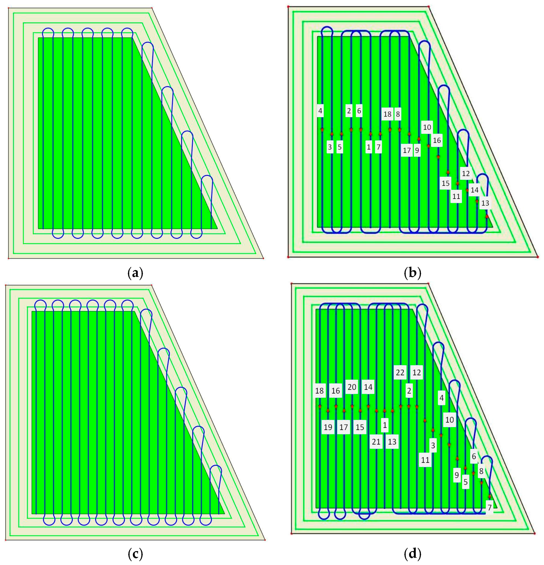
Figure 2.
Representative template field shapes [22].
Figure 2.
Representative template field shapes [22].

Figure 3.
The assessment model structure.
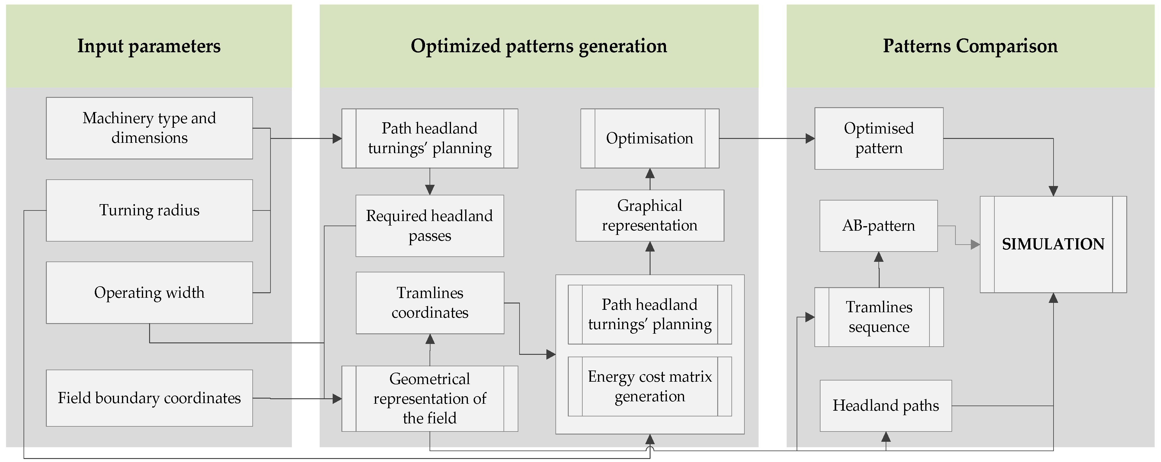
Figure 4.
Total time requirements for each field shape (CS1: Miscanthus; CS2: Switchgrass).

Figure 5.
Savings (%) in fuel energy consumption in the optimised case studies.
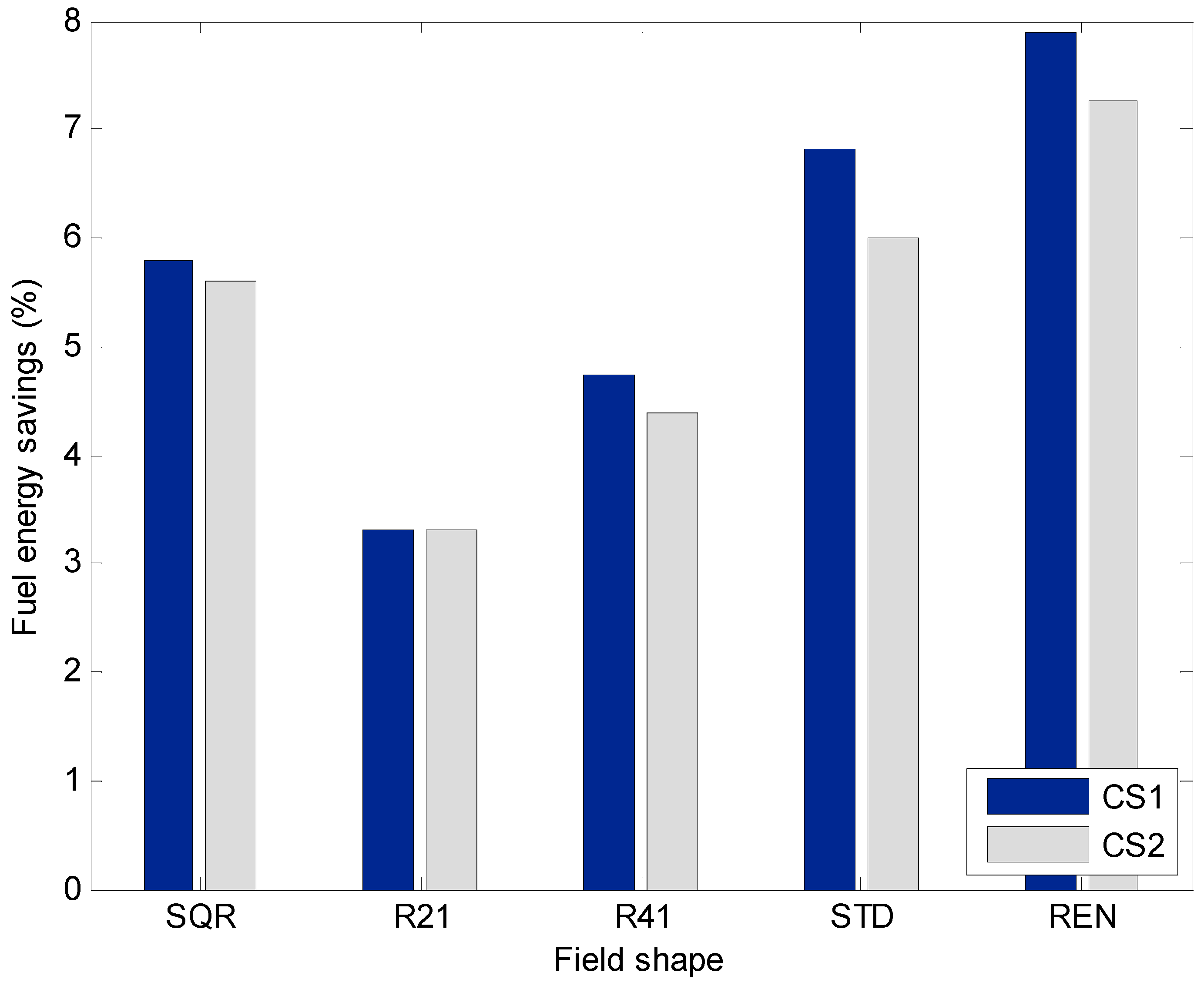
Figure 6.
Embodied energy savings in the optimised case studies.

Figure 7.
Total energy savings in the optimised case studies.
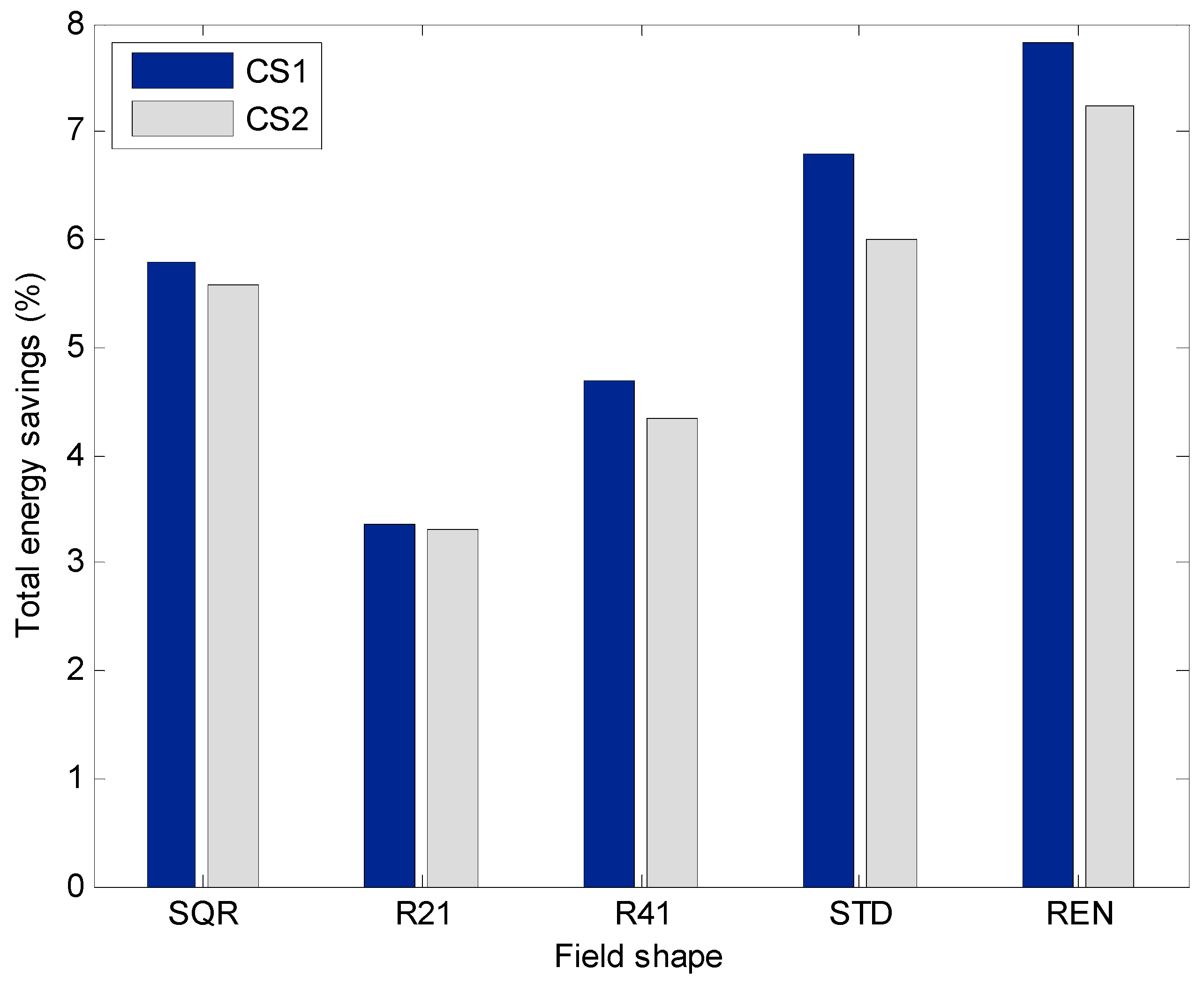
Figure 8.
Energy savings (%) for different tractor sizes in CS1 (case study 1). (S: Small-sized tractor (up to 50 kW); M: Medium-sized tractor (up to 120 kW), and; L: Large-sized tractor (up to 180 kW)).
Figure 8.
Energy savings (%) for different tractor sizes in CS1 (case study 1). (S: Small-sized tractor (up to 50 kW); M: Medium-sized tractor (up to 120 kW), and; L: Large-sized tractor (up to 180 kW)).

Figure 9.
Energy savings (%) for different tractor sizes in CS2 (case study 2) (S: Small-sized tractor (up to 50 kW); M: Medium-sized tractor (up to 120 kW), and; L: Large-sized tractor (up to 180 kW)).
Figure 9.
Energy savings (%) for different tractor sizes in CS2 (case study 2) (S: Small-sized tractor (up to 50 kW); M: Medium-sized tractor (up to 120 kW), and; L: Large-sized tractor (up to 180 kW)).


Table 1.
Field machinery operational characteristics.
| Ploughing | Disk-Harrow | Planting | Spreading | Mowing | Harvesting | ||
|---|---|---|---|---|---|---|---|
| Operating width (m) | CS1 | 3 | 4.5 | 3 | 12 | - | 3 |
| CS2 | 3 | 6 | 4.5 | 10.5 | 3 | 3 | |
| Minimum turning radius (m) | CS1 | 6 | 4.5 | 3 | 6 | - | 6 |
| CS2 | 6 | 4.5 | 3 | 6 | 3 | 6 | |
| Operating speed (m/s) | CS1/CS2 | 2 | 2.8 | 2.5 | 3 | 3 | 1.4 |
CS—Case study.
Table 2.
Field machinery energy inputs per operation.
| Tractor Embodied Energy 1 (MJ·kg−1) | Implement Embodied Energy 1 (MJ·kg−1) | Tractor Mass 2 (103 kg) | Implement Mass 3 (103 kg) | Tractor Estimated Life 4 (103 h) | Implement Estimated Life 4 (103 h) | Tractor Power (kW) | |
|---|---|---|---|---|---|---|---|
| Plough | 138 | 180 | 10 | 2.30 | 16 | 2 | 180 |
| Disk-harrow | 138 | 149 | 6.76 | 1.80 | 16 | 2 | 120 |
| Spreading | 138 | 129 | 10 | 3.35 | 16 | 1.2 | 180 |
| Planting/Seeding | 138 | 133 | 2.93 | 1.20 | 12 | 1.5 | 50 |
| Mowing | 138 | 110 | 6.76 | 0.65 | 16 | 2 | 120 |
| Harvesting | 138 | 116 | 10 | 0.90 | 16 | 2.5 | 180 |
Table 3.
Time requirements (min/ha) per operation for each field shape (SQR-Square, R21-Rectangle 2:1, R41-Rectangle 4:1, STD-Standard, REN-Re-entrant) for the two Case Studies (CS1: Miscanthus; CS2: Switchgrass).
Table 3.
Time requirements (min/ha) per operation for each field shape (SQR-Square, R21-Rectangle 2:1, R41-Rectangle 4:1, STD-Standard, REN-Re-entrant) for the two Case Studies (CS1: Miscanthus; CS2: Switchgrass).
| Field Shape | Case Study | Field Route Planning | Ploughing | Disk-Harrow | Planting | Spreader | Mower | Harvesting |
|---|---|---|---|---|---|---|---|---|
| SQR | CS1 | Non-optimised | 33.3 | 15.7 | 24.7 | 5.8 | - | 46.0 |
| Optimised | 31.2 | 14.6 | 23.4 | 5.6 | - | 43.3 | ||
| CS2 | Non-optimised | 33.3 | 11.8 | 16.7 | 6.7 | 20.3 | 45.8 | |
| Optimised | 31.3 | 11.2 | 16.2 | 6.3 | 19.3 | 43.2 | ||
| R21 | CS1 | Non-optimised | 32.1 | 15.1 | 24.5 | 5.7 | - | 44.2 |
| Optimised | 31.0 | 14.2 | 23.5 | 5.5 | - | 43.0 | ||
| CS2 | Non-optimised | 32.1 | 11.4 | 16.2 | 6.4 | 20.2 | 44.1 | |
| Optimised | 30.9 | 10.9 | 15.7 | 6.0 | 19.4 | 43.2 | ||
| R41 | CS1 | Non-optimised | 31.6 | 15.0 | 24.3 | 5.6 | - | 44.1 |
| Optimised | 30.8 | 14.3 | 23.5 | 5.4 | - | 41.2 | ||
| CS2 | Non-optimised | 31.6 | 11.6 | 16.2 | 6.4 | 20.0 | 44.1 | |
| Optimised | 30.8 | 11.3 | 15.9 | 6.1 | 19.4 | 41.1 | ||
| STD | CS1 | Non-optimised | 33.8 | 16.2 | 24.7 | 5.6 | - | 46.6 |
| Optimised | 31.4 | 14.6 | 23.7 | 5.4 | - | 43.6 | ||
| CS2 | Non-optimised | 33.7 | 11.5 | 16.3 | 6.4 | 20.3 | 46.5 | |
| Optimised | 30.6 | 11.3 | 16.0 | 6.2 | 19.5 | 43.5 | ||
| REN | CS1 | Non-optimised | 35.1 | 15.9 | 25.0 | 5.7 | - | 48.4 |
| Optimised | 31.9 | 14.6 | 23.6 | 5.6 | - | 44.3 | ||
| CS2 | Non-optimised | 35.1 | 11.8 | 16.5 | 6.5 | 20.6 | 48.4 | |
| Optimised | 31.9 | 11.5 | 16.0 | 6.2 | 19.4 | 44.1 |
Table 4.
Fuel energy savings (%) per operation.
| Field Shape | Case Study | Ploughing | Disk-Harrow | Planting | Spreader | Harvesting | Mowing |
|---|---|---|---|---|---|---|---|
| SQR | CS1 | 6.25 | 7.07 | 5.09 | 3.92 | 5.76 | - |
| CS2 | 6.25 | 5.20 | 3.21 | 5.81 | 5.76 | 5.15 | |
| R21 | CS1 | 3.61 | 5.70 | 3.93 | 4.55 | 2.16 | - |
| CS2 | 3.61 | 4.20 | 2.90 | 6.32 | 2.16 | 4.20 | |
| R41 | CS1 | 2.57 | 4.54 | 3.14 | 3.60 | 6.85 | - |
| CS2 | 2.57 | 3.19 | 2.11 | 4.49 | 6.85 | 3.23 | |
| STD | CS1 | 9.18 | 6.57 | 3.95 | 2.83 | 6.52 | - |
| CS2 | 9.19 | 1.70 | 2.13 | 3.81 | 6.52 | 3.91 | |
| REN | CS1 | 9.04 | 8.49 | 5.51 | 1.20 | 8.82 | - |
| CS2 | 9.04 | 2.29 | 2.70 | 3.96 | 8.82 | 5.83 |
Table 5.
Embodied energy savings (%) per operation.
| Field Shape | Case Study | Ploughing | Disk-Harrow | Planting | Spreader | Harvesting | Mowing |
|---|---|---|---|---|---|---|---|
| SQR | CS1 | 6.25 | 7.09 | 5.07 | 3.90 | 5.76 | - |
| CS2 | 6.25 | 5.22 | 3.23 | 5.83 | 5.76 | 5.16 | |
| R21 | CS1 | 3.60 | 5.69 | 3.92 | 4.56 | 2.16 | - |
| CS2 | 3.61 | 4.20 | 2.89 | 6.15 | 2.16 | 4.21 | |
| R41 | CS1 | 2.57 | 4.53 | 3.14 | 3.59 | 6.85 | - |
| CS2 | 2.57 | 3.19 | 2.14 | 4.60 | 6.85 | 3.22 | |
| STD | CS1 | 9.18 | 6.57 | 3.96 | 2.81 | 6.52 | - |
| CS2 | 9.19 | 1.69 | 2.15 | 3.74 | 6.53 | 3.93 | |
| REN | CS1 | 9.04 | 8.50 | 5.50 | 1.21 | 8.82 | - |
| CS2 | 9.04 | 2.31 | 2.66 | 3.87 | 8.83 | 5.84 |
© 2017 by the authors. Licensee MDPI, Basel, Switzerland. This article is an open access article distributed under the terms and conditions of the Creative Commons Attribution (CC BY) license (http://creativecommons.org/licenses/by/4.0/).
Share and Cite
MDPI and ACS Style
Rodias, E.; Berruto, R.; Busato, P.; Bochtis, D.; Sørensen, C.G.; Zhou, K. Energy Savings from Optimised In-Field Route Planning for Agricultural Machinery. Sustainability 2017, 9, 1956. https://doi.org/10.3390/su9111956
AMA Style
Rodias E, Berruto R, Busato P, Bochtis D, Sørensen CG, Zhou K. Energy Savings from Optimised In-Field Route Planning for Agricultural Machinery. Sustainability. 2017; 9(11):1956. https://doi.org/10.3390/su9111956
Chicago/Turabian StyleRodias, Efthymios, Remigio Berruto, Patrizia Busato, Dionysis Bochtis, Claus Grøn Sørensen, and Kun Zhou. 2017. "Energy Savings from Optimised In-Field Route Planning for Agricultural Machinery" Sustainability 9, no. 11: 1956. https://doi.org/10.3390/su9111956
Note that from the first issue of 2016, this journal uses article numbers instead of page numbers. See further details here.