Reference Evapotranspiration Retrievals from a Mesoscale Model Based Weather Variables for Soil Moisture Deficit Estimation

Abstract

Reference Evapotranspiration (ETo) and soil moisture deficit (SMD) are vital for understanding the hydrological processes, particularly in the context of sustainable water use efficiency in the globe. Precise estimation of ETo and SMD are required for developing appropriate forecasting systems, in hydrological modeling and also in precision agriculture. In this study, the surface temperature downscaled from Weather Research and Forecasting (WRF) model is used to estimate ETo using the boundary conditions that are provided by the European Center for Medium Range Weather Forecast (ECMWF). In order to understand the performance, the Hamon’s method is employed to estimate the ETo using the temperature from meteorological station and WRF derived variables. After estimating the ETo, a range of linear and non-linear models is utilized to retrieve SMD. The performance statistics such as RMSE, %Bias, and Nash Sutcliffe Efficiency (NSE) indicates that the exponential model (RMSE = 0.226; %Bias = −0.077; NSE = 0.616) is efficient for SMD estimation by using the Observed ETo in comparison to the other linear and non-linear models (RMSE range = 0.019–0.667; %Bias range = 2.821–6.894; NSE = 0.013–0.419) used in this study. On the other hand, in the scenario where SMD is estimated using WRF downscaled meteorological variables based ETo, the linear model is found promising (RMSE = 0.017; %Bias = 5.280; NSE = 0.448) as compared to the non-linear models (RMSE range = 0.022–0.707; %Bias range = −0.207–−6.088; NSE range = 0.013–0.149). Our findings also suggest that all the models are performing better during the growing season (RMSE range = 0.024–0.025; %Bias range = −4.982–−3.431; r = 0.245–0.281) than the non−growing season (RMSE range = 0.011–0.12; %Bias range = 33.073–32.701; r = 0.161–0.244) for SMD estimation.

1. Introduction

Local, regional, or global scale monitoring of Reference Evapotranspiration (or ETo) is vital for assessing climate and human-induced affects on natural and agricultural ecosystems and for developing a sustainable environment using efficiently the Earth’s resources [1,2,3,4]. There are numerous methods available for assessment of ET based on different conditions of soil, water, plants, and land cover [5,6,7,8,9]. In 1998, [10] provided a standard method for ET estimation using the standardised FAO-56 Penman-Monteith model for grasses and given the term reference evapotranspiration or ETo. ETo can be represented as the sum of water that can be evaporated from the soil surface and transpired from vegetation when the soil water is sufficient to meet the atmospheric demand [10]. Many studies already have documented that ETo fluxes at various scales have direct effect on water balance and hydrological cycle [11,12]. The regional variations in ETo also influence the soil water content and irrigation water demand [13]. Therefore, accurate estimation of ETo is needed for an improved monitoring of climate, water resources, drought, and flood [14,15].

Evapotranspiration is difficult to measure and indirect procedures through correlations with meteorological factors are generally used. In this direction, there are many methods available to estimate ETo and available in technical literature domain [16]. The available methods for evapotranspiration require complicated computational procedures or the applications of corrective factors that vary with season and location. In this regard, Hamon’s proposed [17] a simple procedure to estimate potential evapotranspiration, in which the available temperature data from various resources can be used. Hamon’s method requires temperature data for calculation of ETo, which can be downscaled using the advanced numerical weather prediction (NWP) model, such as the Weather Research and Forecasting (WRF) model. WRF model is well tested by a number of users with satisfactory performance and hence used in this study for dynamical downscaling of surface temperature [18,19,20,21].

In real conditions, the soil water content usually varies because of changing meteorological conditions, crop suction, and evaporation losses from the soil surface. The amount of water content required to bring back the soil moisture to field capacity can be described by using the term Soil Moisture Deficit (SMD) [22,23]. SMD is an important variable and the prolonged deficiency of SMD leads to drought conditions, while very low SMD may cause flooding problem during extreme rain events. Moreover, monitoring of SMD is an alternative method for irrigation scheduling and represents the usage of an optimal amount of water at appropriate time to avoid any agricultural losses [24]. Potential ET (or PET) models are easy to implement, as they need less complex relations as compared to the actual ET models. Even though several complex surface energy balance models have been developed to map actual ET, these models may not capture extreme soil stress conditions due to a large uncertainties associated with the use of data from multiple sources (i.e., remote sensing, weather station) and assumptions made in these models [25]. The study of [25] indicated that the actual ET models’ performances are strikingly poor in extremely dry conditions. Hence, the use of PET models, such as Hamon’s method and the regression approach, may have a slight advantage over the actual ET models. The empirical approach could capture extreme dry conditions if the models are well constructed by controlling different factors that affect soil moisture. The relationship between the SMD, ETo, rainfall etc is well documented in the previous studies [24,26]. ETo can be used for estimation of SMD by using the appropriate models. Therefore, the main motivation of this study is to monitor the SMD by using the data of ETo estimated from simpler method as given by Hamon’s [17].

In purview of the above, this work is focused on the following objectives: (1) to perform a performance evaluation of the WRF downscaled temperature for ETo estimation; (2) to derive SMD using the WRF and observed ETo through several linear and non-linear models; and, (3) to evaluate the effect of seasonality on SMD retrieval with special reference to growing and non-growing season. This article is divided into following sub-sections. After introduction, Section 2 provides a description of the study area, datasets, theoretical backgrounds of WRF-Noah LSM model, probability distributed model, Hamon’s method, and the methodology adopted to evaluate the method. Section 3 delivers the results and provides a discussion of those in the context of the available literature, followed by the conclusions in Section 4.

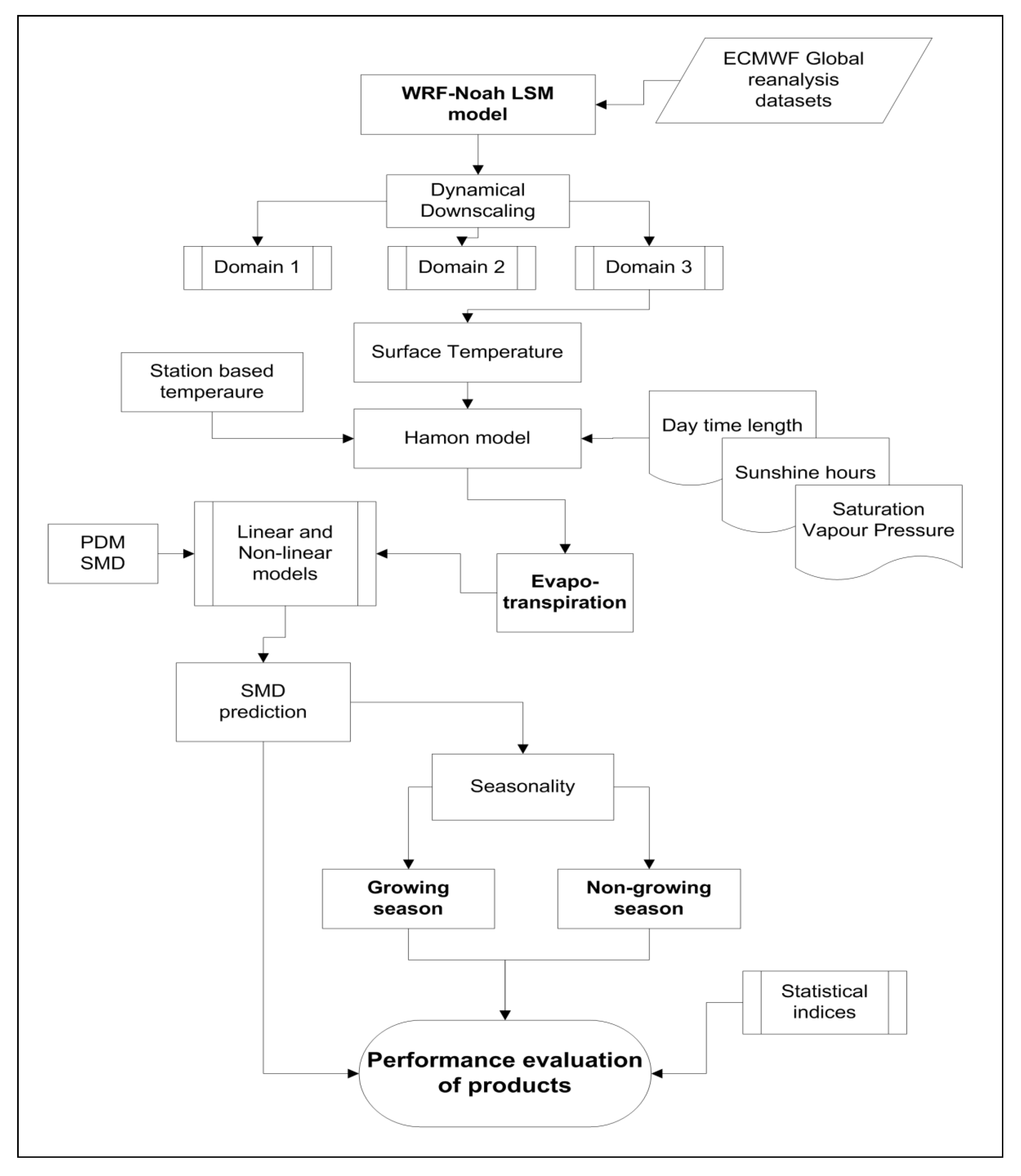
2. Materials and Methods

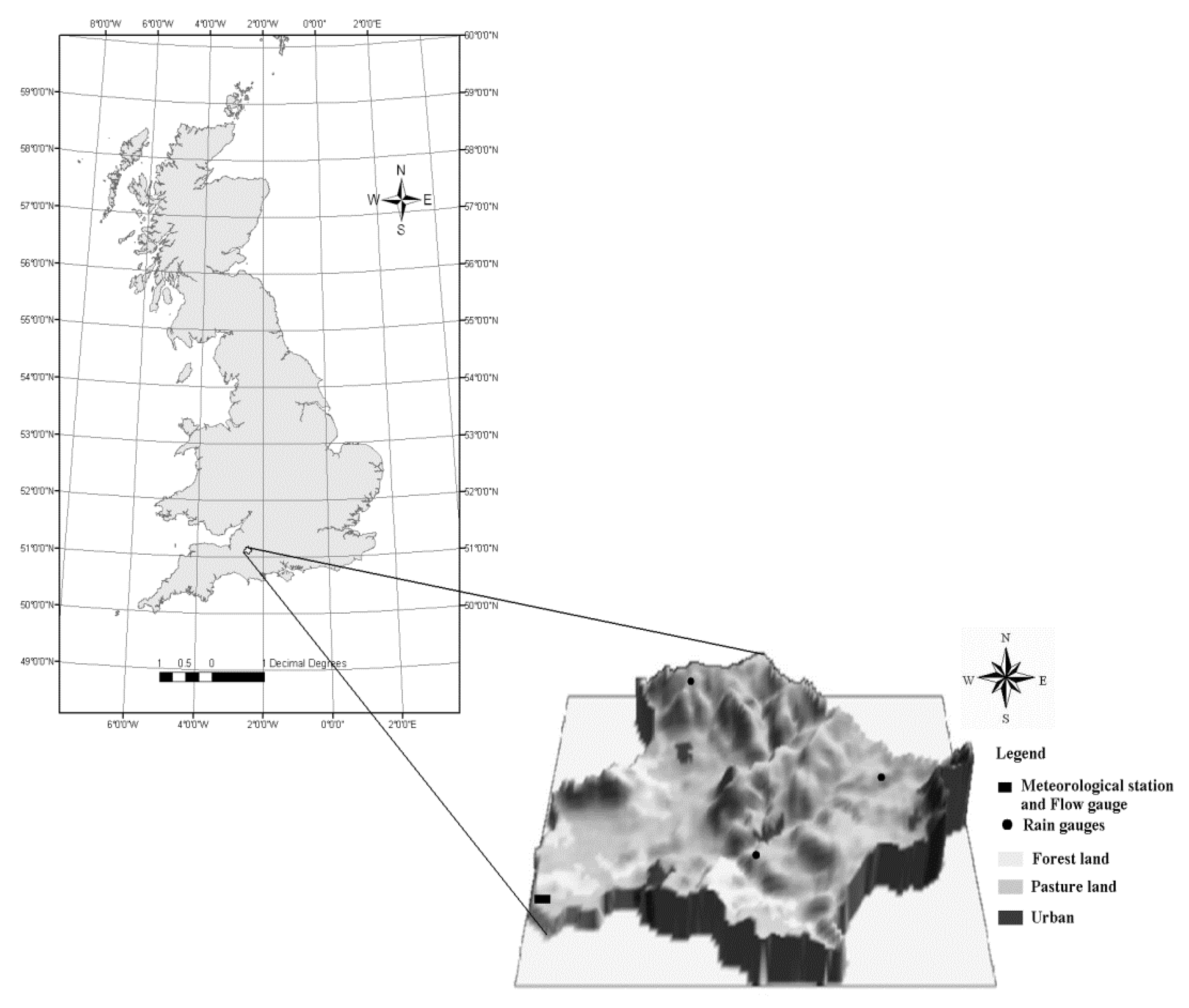
2.1. Study Area and Datasets

The Brue catchment (135.5 km²) is used as a study area, having an elevation of 105 m above mean sea level, positioned in the south-west of England (51.11° N and 2.47° W) (Figure 1). Land use/land cover of the area comprises of pastureland (94.34%), followed by forest (3.48%), and urban settlements (2.18%). It is a predominantly a rural catchment with spring-fed headwaters rising in the Mendip Hills and Salisbury Plain. The DEM created from Digimap, an EDINA service (data library service at the University of Edinburgh) UK. indicates that most of the area shows a modest relief and hence comes under non-complex topography area. The high-resolution soil texture map from LandIS (national computerised database system) of Soil Survey and Land Research Centre (SSLRC) indicates that the most of the area comprises of clayey soil type (49%), followed by coarse loam 29%, and silt 21%. All of the required station based dataset were provided by the Natural Environment Research Council and the British Atmospheric Data Centre, United Kingdom for the calculation of ETo and SMD. For benchmark SMD, a probability distributed model or PDM is employed using the locally measured flow, rainfall, and Evapotranspiration. PDM is used in the UK for both operational and design purposes and successfully employed in other parts of the world [27,28]. The calibration of the model involves two years of hourly data from 1 February 2009 to 31 January 2011 is used, while for validation, one year of data is taken into account for the period 1 February 2011 to 31 January 2012. The SMD obtained during the validation is considered for all of the models development. The overall analysis of PDM indicated a satisfactory performance with NSE value of 0.84 and 0.81 during the calibration and validation respectively. The detailed information on PDM calibration, validation, sensitivity, and uncertainty analysis over Brue is reported in [26]. An overview of the methodology adopted in present study is depicted in Figure 2.

2.2. WRF-Noah LSM Downscaling of Surface Temperature

The WRF-Noah Land Surface Model (LSM), which is based on eta-coordinate modeling system, is used for downscaling surface temperature from ECMWF Re-Analysis (ERA: ECMWF Re-Analysis) interim global reanalysis dataset. In total, 28 terrain following the eta levels in the vertical direction from surface are used following a two-way nesting scheme [29,30]. The WRF physical scheme is shown through

Table 1. WRF physical scheme.

Initial conditions	Three-dimensional real-data (1° × 1° FNL)
Map projection	Lambert
Central point of Domain	Central Latitude: 51.11° N; Central longitude: 2.47° E
Domain	Three Domains
Horizontal grid distribution	Arakawa C-grid
Horizontal grid distance	Domain 3 (9 km)
NCEP Time interval	6 hr
Model output	Hourly
Nesting	2 way
Time integration	3rd-order Runge-Kutta
Spatial differencing scheme	6th-order centered differencing
Lateral boundary condition	Specified options for real-data
Top boundary condition	Gravity wave absorbing (diffusion or Rayleigh damping)
Bottom boundary condition	Physical or free-slip
Microphysics	Lin
Radiation scheme	Dudhia’s short wave radiation/RRTM long wave
Surface layer parameterization	Thermal diffusion scheme
Cumulus parameterization schemes	Betts-Miller-Janjic
PBL parameterization	YSU scheme
Vertical coordinate	Terrain following hydrostatic pressure coordinate ( 28 sigma levels up to 1 hPa )

. The WRF-Noah LSM includes an explicit canopy resistance design given by [31], and a surface runoff scheme is provided by [32]. A comprehensive explanation of the WRF-Noah LSM can be found in [33]. The WRF-Noah LSM model is used with three nested provinces having horizontal grid resolutions of 81 km (D1), 27 km (D2), and 9 km (D3). The D1, D2, and D3 consist of 18 × 18, 19 × 19, and 22 × 22 horizontal grids, respectively. The area with 9 km resolution is used after dynamical downscaling, as others also found that WRF dynamical downscaling improves the estimation of weather data from global reanalysis datasets [34,35,36].

2.3. Probability Distributed Model and Soil Moisture Deficit

The Probability Distributed Model (PDM) comes under the category of lumped model for depicting rainfall runoff relationship developed by the Centre of Ecology and Hydrology (CEH) Wallingford. It is employed in this study for SMD simulation using the ground based inputs of rainfall and reference evapotranspiration (ETo) [28]. It has a better representation of soil moisture computation and is equipped with appropriate time steps for hydrological modelling. Through this model, the SMD can be estimated using the relationship below [37]:

$$\frac{E_i^{\prime }}{E_i}=1-{\left\{\frac{\left(S_{\max }-S(t)\right)}{S_{\max }}\right\}}^{b_e}$$

(1)

where $\frac{E_i^{\prime }}{E_i}$ is the ratio of actual ET to potential ET; and $\left(S_{\max }-S(t)\right)$ is Soil Moisture Deficit; b_e is an exponent in the actual evaporation function; $S_{\max }$ is the total available storage; and, $S(t)$ is storage at a particular time t. The model structure of PDM is further discussed in [37]. Sensitivity analysis (SA) and uncertainty analysis (UA) are considered important to explore the high dimensional parameter spaces, structural uncertainty, and also to understand the sources of uncertainty [38,39].

After a rigorous and careful calibration of the PDM following the Generalized Likelihood Uncertainty Estimation (GLUE), the SMD is extracted. The model parameters for PDM calibration are provided in the study conducted by [29].

2.4. Reference Evapotranspiration or ETo

The study site is predominantly grassland with short green cover of uniform height, completely shading the ground, and with adequate water status in the soil profile. In the case of grasslands, ETo closely resembles the physical condition, as described for PET. Hence, at grassland, both PET and ETo can be safely assumed as equivalent to each other (see the FAO56 criteria for ETo and PET). Many studies have confirmed that Hamon provides a stable and reasonable output as compared to the Thornthwaite, Hargreaves, and Samani methods [40,41], therefore it is also used in the current study to estimate the ETo. Hamon [17] proposed an equation to calculate ETo by providing day length and mean air temperature [42]. It shows the relationships among potential evapotranspiration, saturation vapor pressure, and the possible incoming radiant energy by means of the prevailing air temperature. The hours of sunlight can be used as an index for the maximum possible incoming radiant energy, while the absolute humidity at saturation is used for the estimating the moisture-holding capacity of air. It uses the mean daily temperature and sunshine hours for ETo calculation. The saturation vapor pressure, e_s, is then determined directly from the mean air temperature. One typical feature of this method is that when mean air temperature is lesser than 0 °C, the ETo does not drop up to zero; instead, it provides effectively the same as annual total of the Thornthwaite method [6]. In the Hamon technique, ETo (mm/day) is estimated as follows:

$$ETo\text{ }=29.8\times L_{day}\left(\frac{e_s}{T+273.3}\right)$$

(2)

where: T = Temperature (degree centigrade); $L_{day}=$ Day time length (Unitless); $e_s$ Saturation Vapor Pressure (mb) at given T can be computed using:

$$e_s={6.108}_e\left(\frac{17.27T}{T+273.3}\right)$$

(3)

The $L_{day}$ was obtained from the website http://www.soda-pro.com/ by providing the information of solar declination and latitude. The observed ETo is calculated by using the station based dataset following the Hamon’s method as described above.

2.5. Performance Analysis

In the present study, SMD assessed from the WRF and observed ETo are validated with PDM SMD. The performance statistics Nash Sutcliffe Efficiency (NSE) [43], Root Mean Square Error (RMSE), and %Bias and Correlation (r) are used to understand the model performances. The %Bias, NSE, and RMSE can be calculated using Equations (4)–(6).

$$\%Bias=100\times [{\displaystyle \sum (y_i-x_i)}/{\displaystyle \sum (x_i)}]$$

(4)

$$NSE=1-\frac{{\displaystyle \sum _{i-1}^n{\left[y_i-x_i\right]}^2}}{{\displaystyle \sum _{i-1}^n{\left[x_i-{\overline{x}}_i\right]}^2}}$$

(5)

$$RMSE=\sqrt{\left(\frac{1}{n}{\displaystyle \sum _{i=1}^n{\left[y_i-x_i\right]}^2}\right)}$$

(6)

where n is the number of observations; x is the perceived variable and y is the simulated variable.

3. Results & Discussion

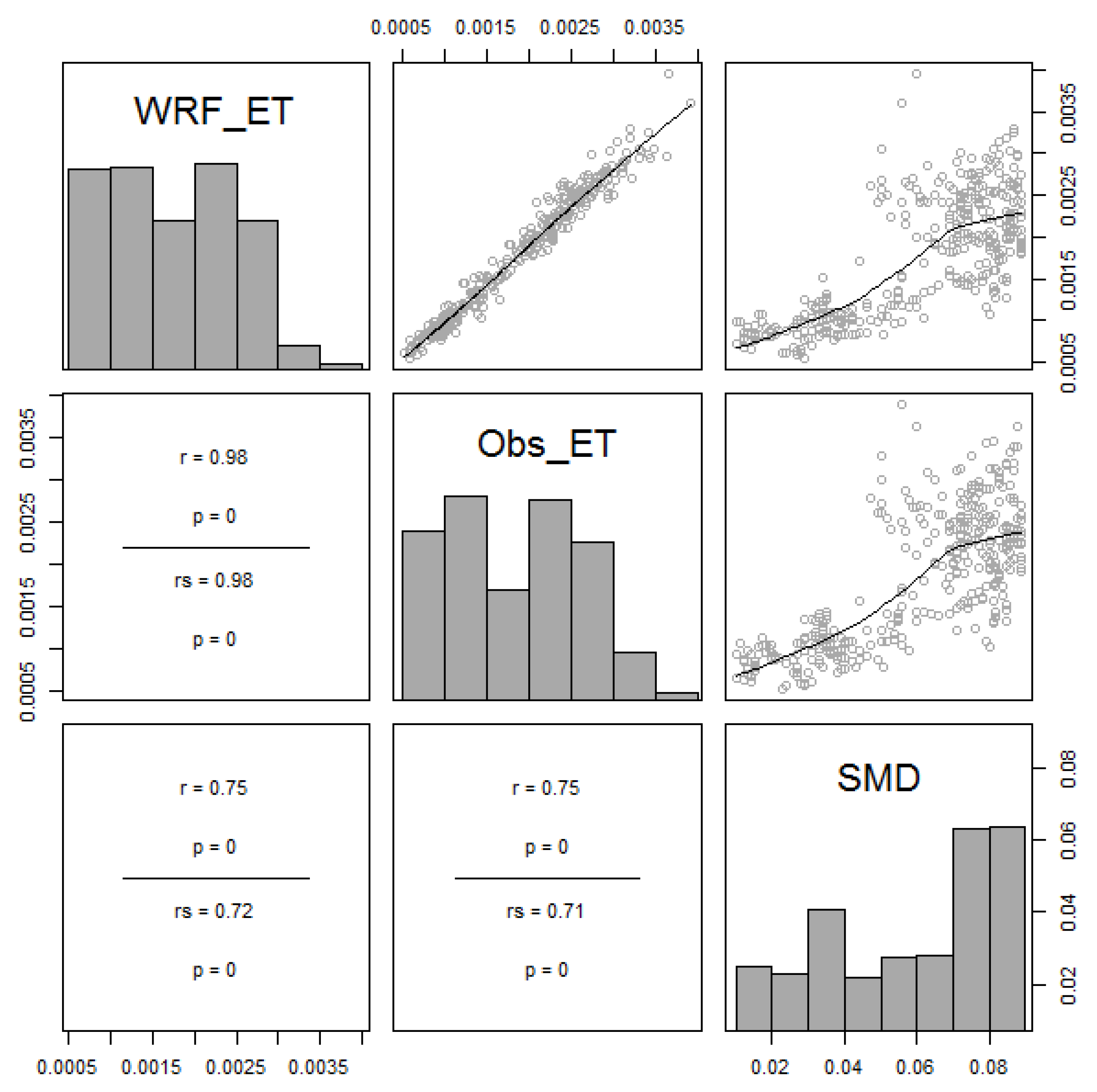
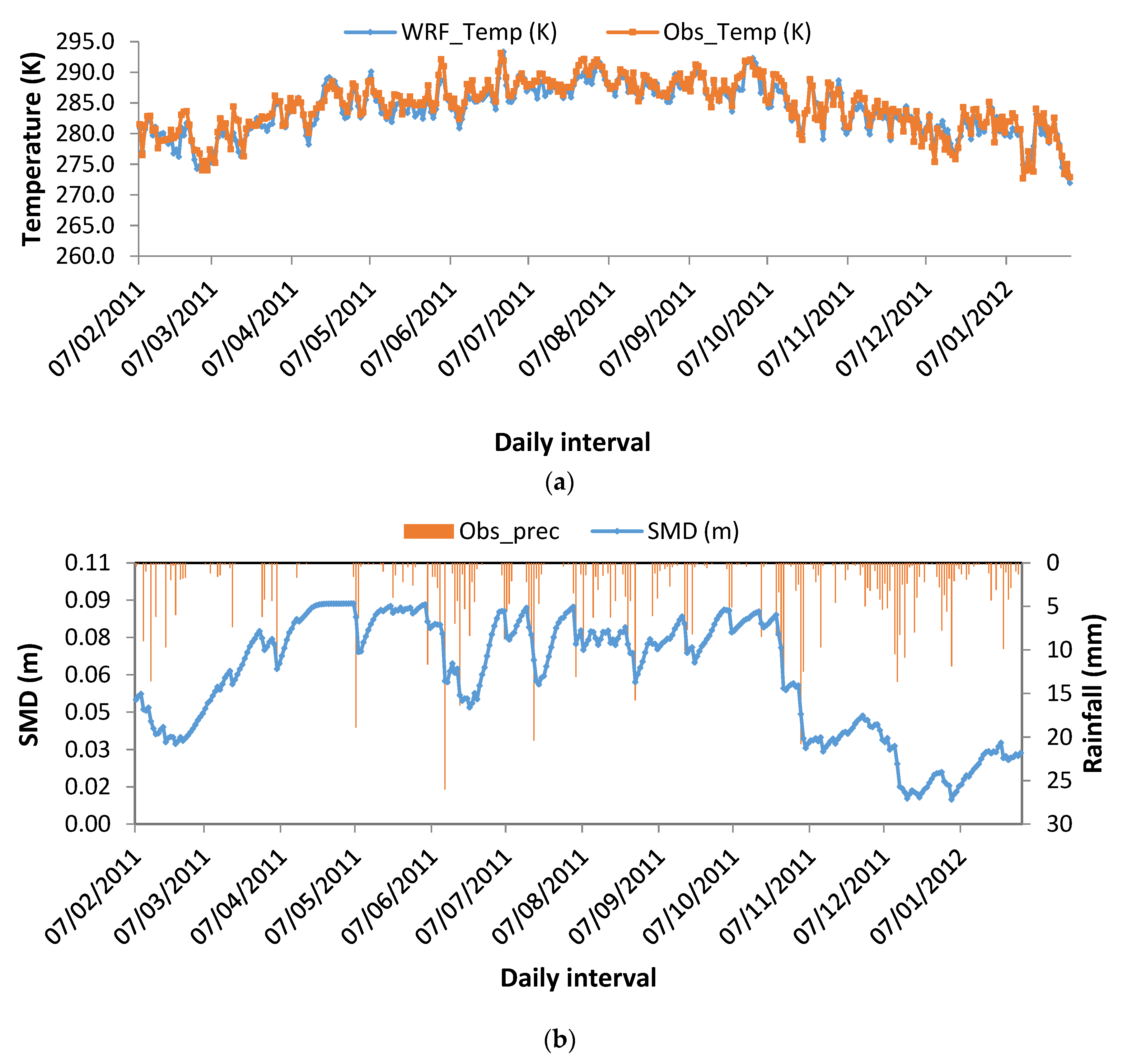
3.1. Evaluation of Hydro-Meteorological Variables

The WRF-Noah LSM downscaled temperature data is evaluated by utilising the observed temperature measured at the meteorological station. The trends in the WRF and observed temperature are represented through Figure 3a, while the association between the SMD and rainfall are indicated in Figure 3b. Both of the plots are used to understand the relationship between the SMD behavior and the hydro-meteorological parameters (rainfall and temperature). A direct appraisal of the temperatures from WRF with the other hydro-meteorological variables showed that these results are comparable to those obtained in the past and with the other data sets collected in this catchment. The analysis of WRF estimated and observed temperature showed a strong correlation of 0.95 between both datasets. In spite of some minor mismatches in the data, the plot indicates a general covenant between the temporal trend of the WRF and observed temperatures with seasons and the declining trend of the rainfall throughout the observation period. A significant optimistic relationship between the SMD and temperature are also evident in the Figure 3a,b. All of the plots exhibit a close match with the seasonal changes from winter to autumn. There is a gradual rise in temperature observed, when progressing from the winter to spring and summer seasons, followed by gradual decrease in temperature on arrival of the autumn season. Similar behavior can be seen in the SMD pattern also, as a rise in temperature causes an increase in SMD values. Some spikes in the temporal plots can be attributed to some sporadic rainfall or storm events. These short duration storms cause a change in SMD and create spiky fluctuations in temperature. It is also evident from the figure that after a rainfall event, there is some lag time for SMD changes for nearly ~1–2 days. Therefore, in overall, there are significant relationships that exist between the temperature and the SMD in the Brue catchment.

The ETo, calculated by using the temperature data from WRF and ground based observations, are shown using the correlation matrix plots along with the SMD in Figure 4. Hydro-meteorological variables used for ETo estimation are temperature, sunshine hour, and saturation vapor pressure following the Hamon method. The Hamon model is grounded on coefficient derived from an empirically determined model. The time series of both the observed and WRF ETo are ranges from 0.0005 mm/day to 0.0040 mm/day. There is a no major difference found between the WRF and the observed dataset when plotted against SMD. The r and rs correlations indicates a value of 0.75 for both WRF and observed ETo, which indicates that the WRF downscaled surface temperature when used with Hamon method can provide an accurate estimates of ETo for various applications. Some lower performances in correlation can be attributed to the high precipitation in the Brue catchment and the influence of temperate maritime climate. Further, slight overestimation of ETo over wet areas indicates that a correction factor is needed in the Hamon model.

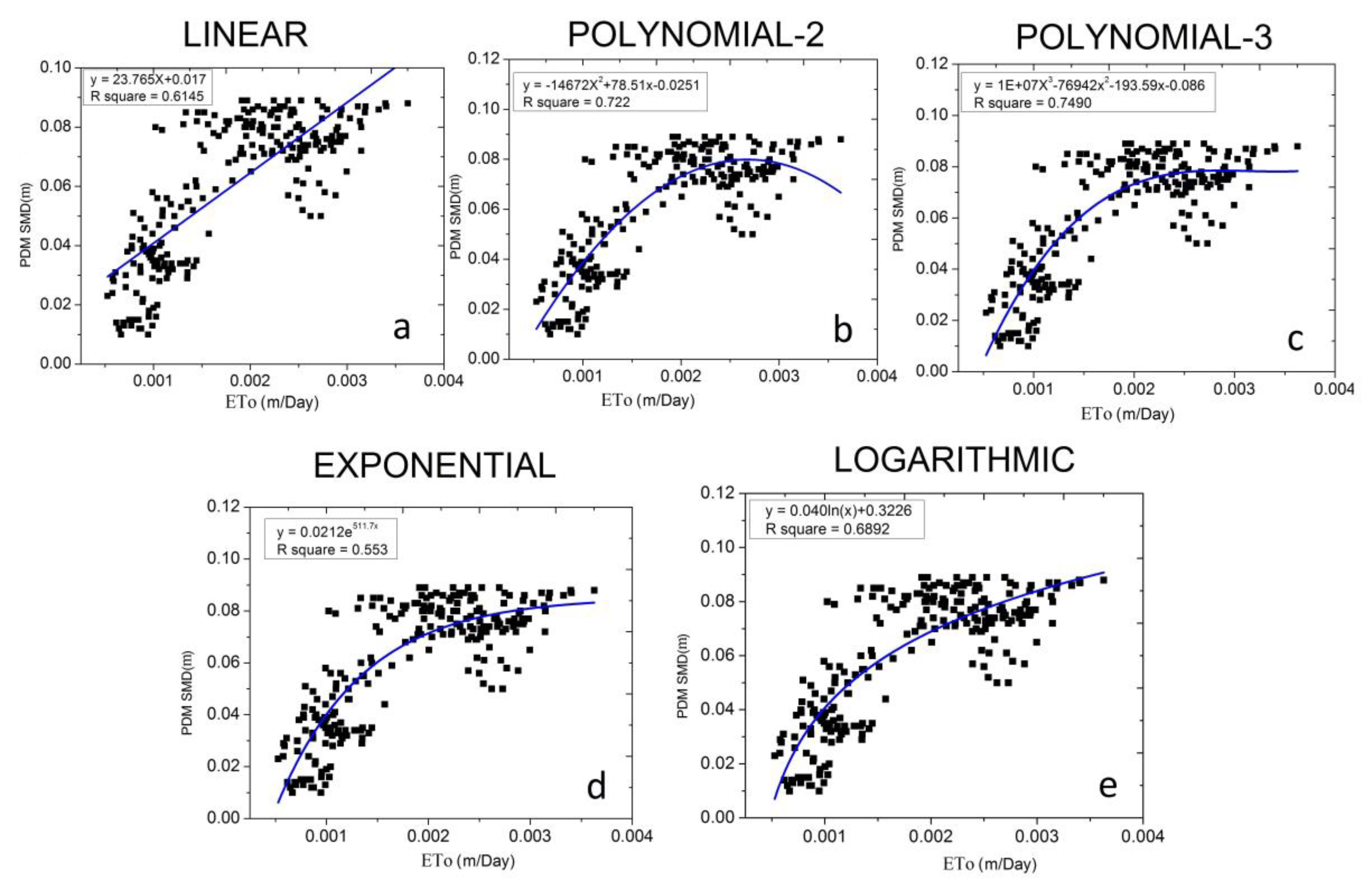
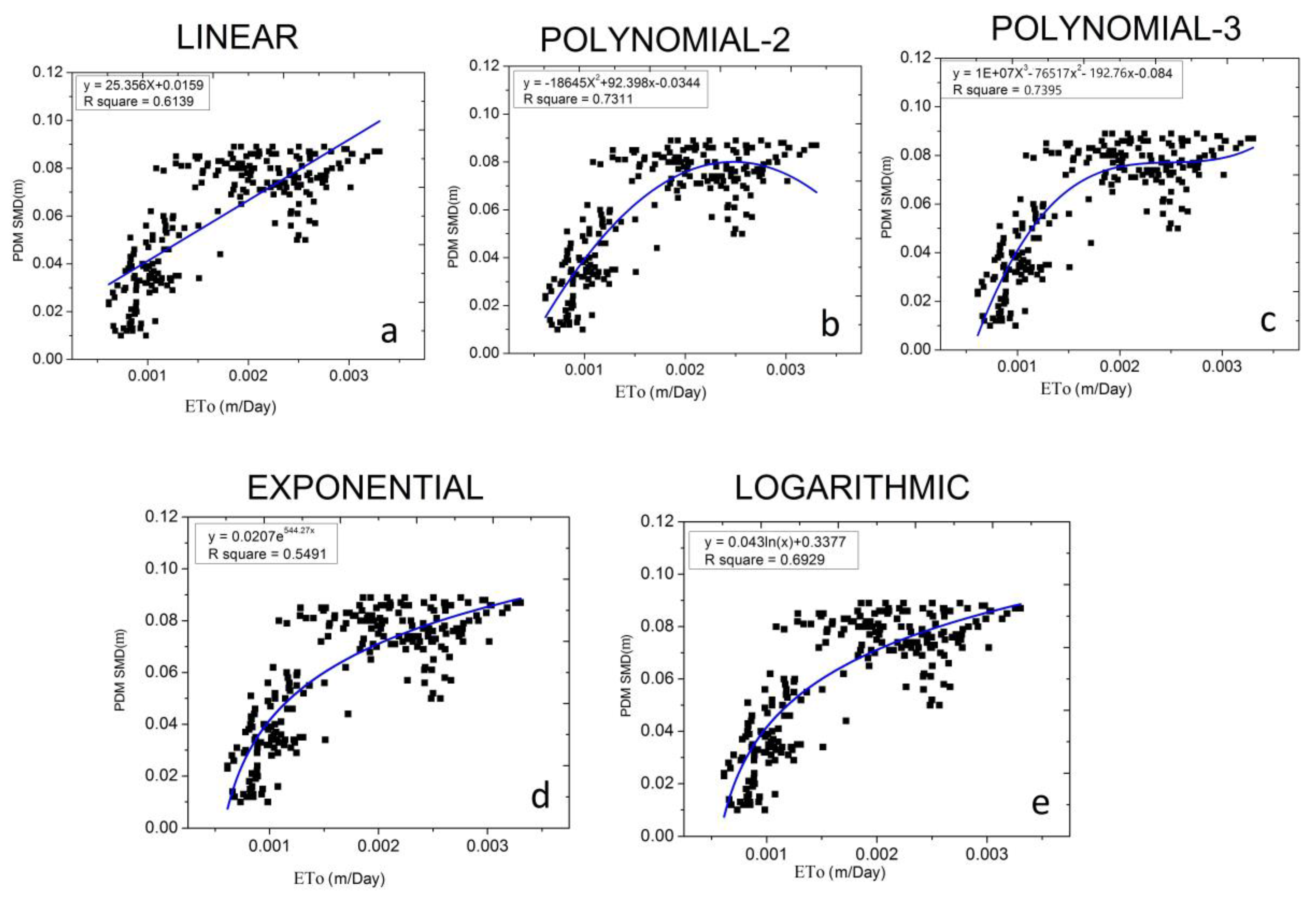
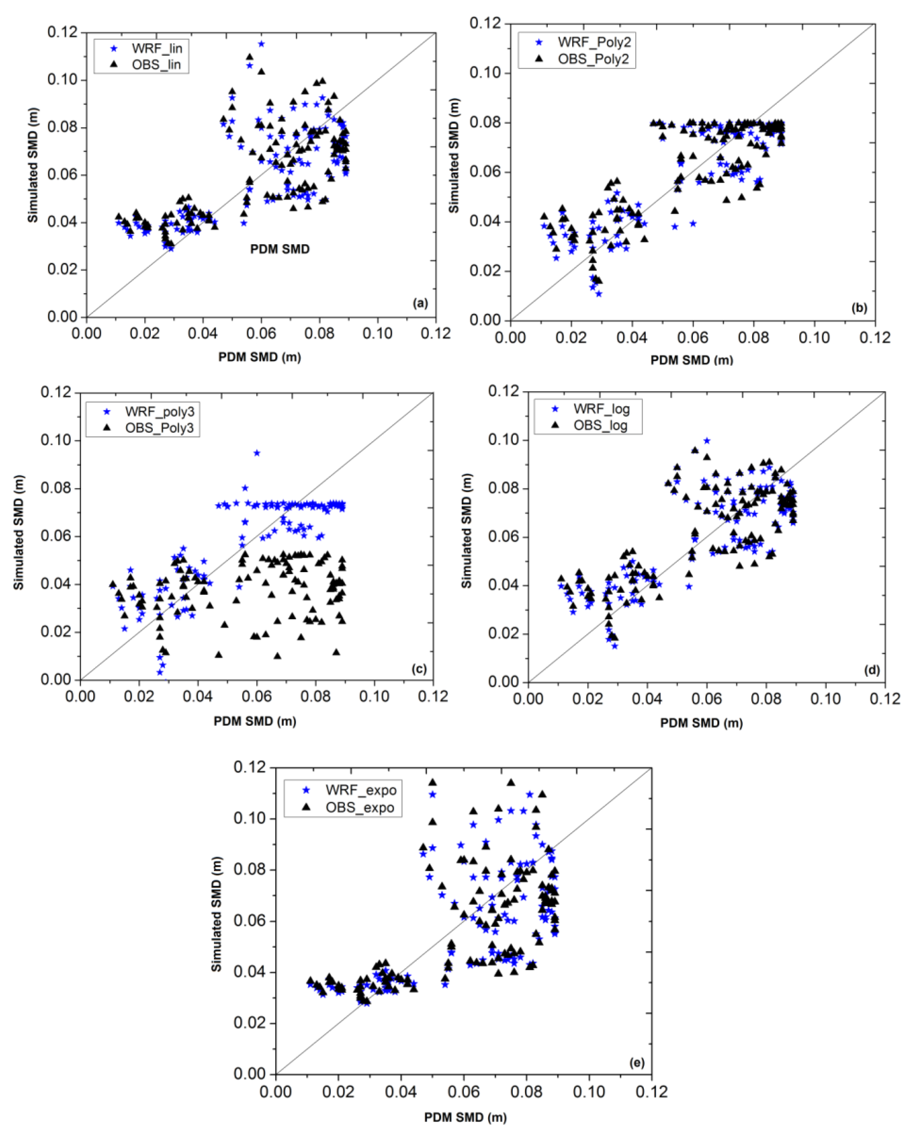
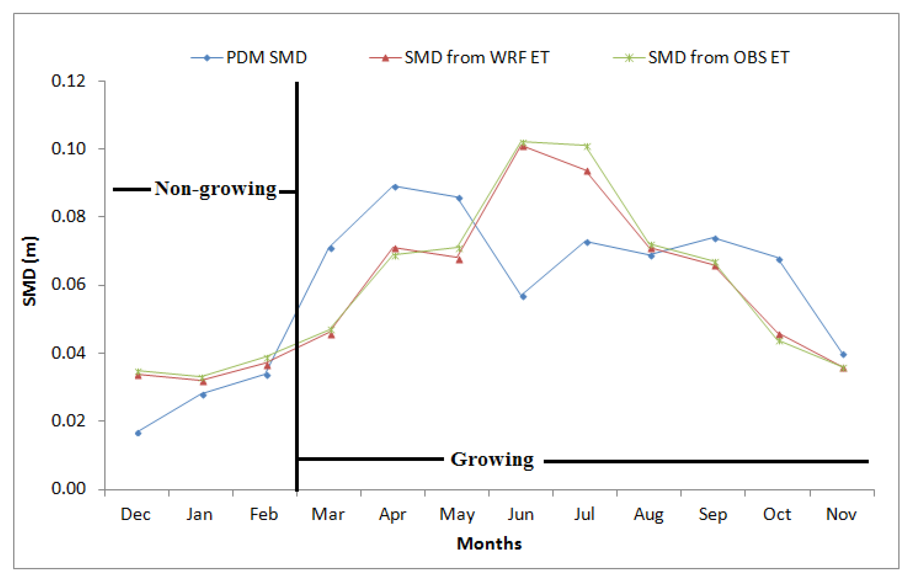
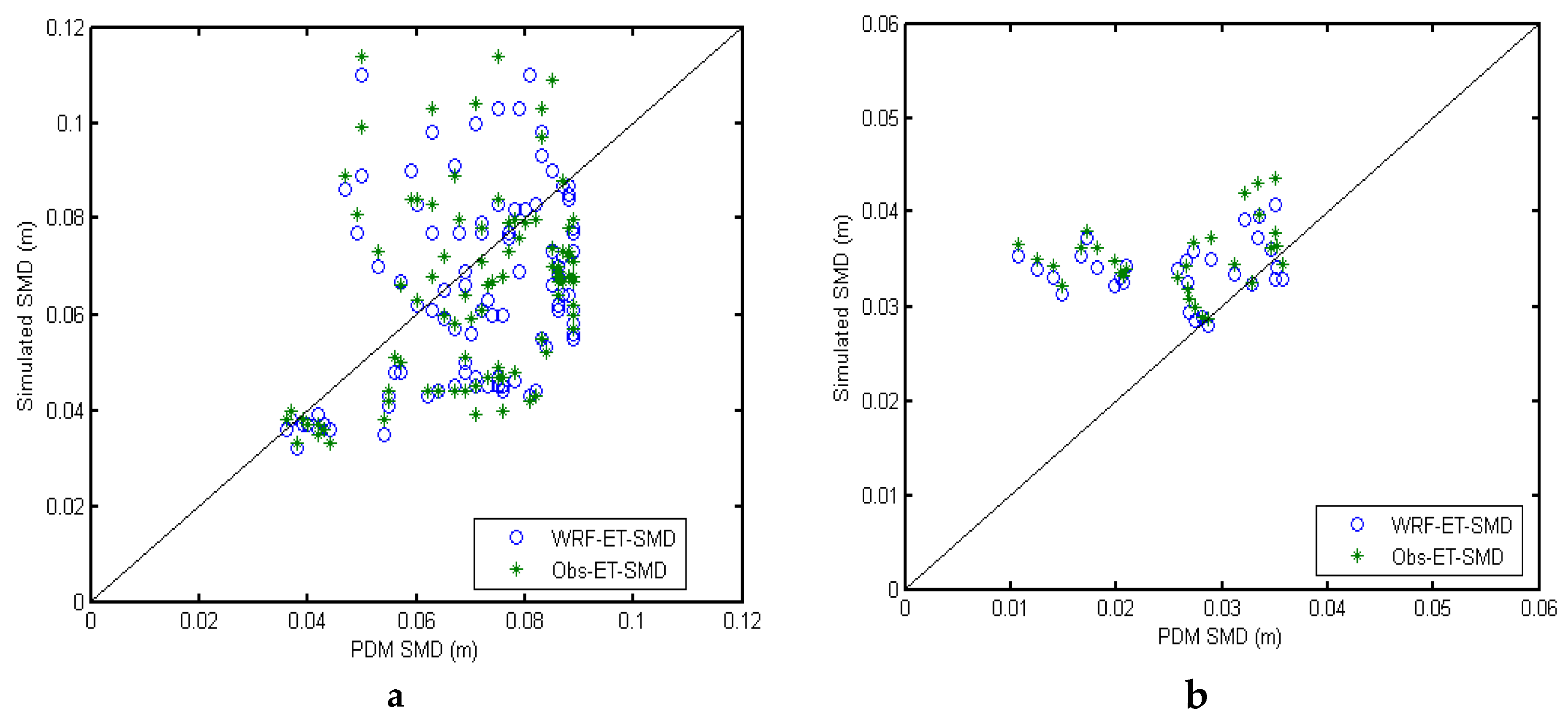
3.2. Comparison of SMD Estimated Using Different ETo Products

For utilization of dataset for hydrological applications, the relationship between PDM and ETo based SMD is examined using various linear and nonlinear algorithms. To segregate the data for calibration and validation, the dataset is distributed into two-third and one-third parts. The first two third parts are considered for model calibrations, while the remaining part is for the models validation. This method has its own significance as it represents the data for all of the seasons. In total, five linear and non-linear models are employed to estimate the relationships for SMD assessment using the perceived and WRF ETo viz linear, second and third order polynomial, exponential, and logarithmic algorithms (Figure 5 and Figure 6). In

Table 2. Different models used for SMD estimation using WRF and Observed ETo.

S. No.	Model	Observed ETo and SMD		WRF ETo and SMD
		Equation	R2	Equation	R2
1	Linear	23.765X + 0.017	0.614	25.356X + 0.016	0.614
2	Polynomial 2	−14672X2 + 78.51X − 0.025	0.722	−18645X2 + 92.398X − 0.034	0.731
3	Polynomial 3	1E + 07X3 − 76942X2 − 193.59X − 0.086	0.749	1E + 07X3 − 76517X2 − 192.76X − 0.084	0.739
4	Logarithmic	0.040ln(X) + 0.323	0.689	0.043ln(X) + 0.338	0.693
5	Exponential	0.0212e511.7X	0.553	0.0207e544.27X	0.549

, the performances of the diverse models in terms of R² are indicated by using the ETo derived from WRF and Observed dataset. The model results indicate that the observed ETo and SMD indicate a higher performance in comparison to WRF ETo. Among all of the techniques, 0.749 is the best NSE obtained with 3rd order polynomial regression technique, implies that the relationship between PDM, SMD, and observed ETo can be best represented by third order polynomial. Other than this logarithmic and second order polynomial models are also produced satisfactory R² values of 0.689 and 0.722 respectively. On the other hand, the linear and exponential model does not provide good results as compared to other techniques. The performance statistics between WRF ETo and PDM SMD indicates a marginally lower performance in contrast to the observed ETo (Table 2). As expected, in the case of WRF, the R² for different regression techniques gives the similar values, as observed ones with the highest in case of 3rd order polynomial (0.739) followed by 2nd order polynomial (0.731), logarithmic (0.689), exponential (0.549), and linear (0.616) during the calibration. It is evident from the R² statistics that WRF simulated surface temperature data could be used for SMD in absence of ground-based observations. However, an exact accuracy of the dataset is needed for operational applications. The validations of linear and non-linear models for SMD estimation are presented with their performance statistics in

Table 3. Performance of models during validation.

S. No.	Model	Observed ETo and SMD			WRF ETo and SMD
		RMSE	%Bias	NSE	RMSE	%Bias	NSE
1	Linear	0.019	5.149	0.419	0.017	5.280	0.448
2	Polynomial 2	0.667	3.568	0.013	0.707	1.934	0.013
3	Polynomial 3	0.627	2.821	0.014	0.679	−0.207	0.013
4	Logarithmic	0.535	6.894	0.016	0.589	2.744	0.015
5	Exponential	0.226	−0.077	0.616	0.022	−6.088	0.149

. The statistical indices such as NSE, RMSE, and %Bias test are used to understand the model performances during the validation, while the behavior of the dataset can be seen in Figure 7. Different algorithms provide different NSE values, which ranges from 0.013 to 0.448. From the results, it is evident that the linear regression technique has good NSE (0.448) as compared to all of the other models. The high performance of linear model herein can be revealed by analyzing the Pearson’s and Spearman’s correlation statistics between PDM SMD, observed and WRF ETo. From the Spearman’s correlation statistics, it is clear that that there is no strong non-linearity exists between the dataset and therefore, the proposed linear model could be used for SMD estimation, because of its simplicity.

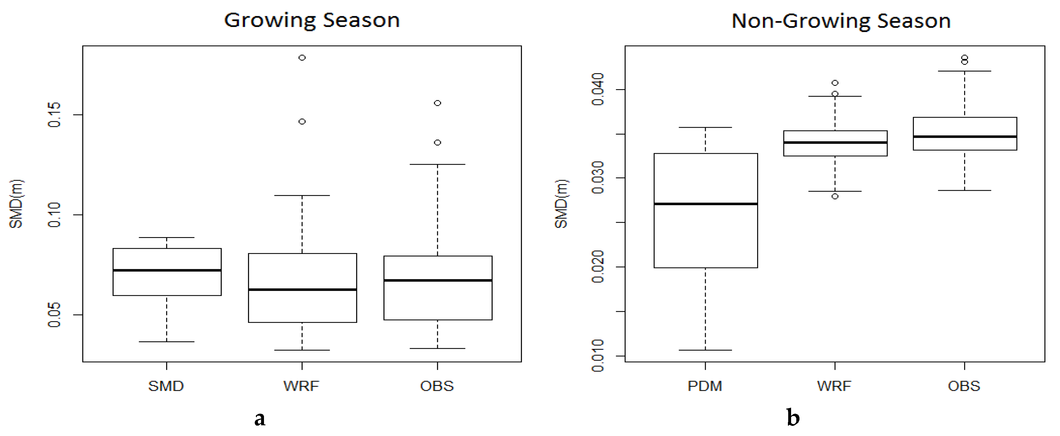
3.3. Performance with Growing and Non-Growing Seasons

Many studies indicated that vegetation plays an important role in the differences of soil water content. Authors have reported that the transformation in seasons specially growing and non-growing season have significant impact on SMD. In an earlier study, it has been found that growing and non-growing seasons behave differently. Therefore, for proper assessment and understanding of SMD inclusion of growing and non-growing seasons are important. During the growing season, crops create problems in the estimation of actual values of ETo, as they do not have a proper correction factor to differentiate between the growing and non-growing seasons. For understanding the data in an efficient way, the dataset is divided conferring to the growing and non-growing seasons. As per the UK met office, temperature is an important parameter for deciding the growing and non-growing seasons. When the temperature of five consecutive days exceeds 5 °C, there will be an onset of growing season, while it ends when the temperatures fall below 5 °C for five consecutive days [27]. The 1971 to 2000 average season length was 280 days (~9.3 months) (Source: http://www.metoffice.gov.uk/climate/uk/averages/ukmapavge.html). Therefore, in the current study, the entire season of winter (December–February) is taken as non-growing (average temperature < 5 °C), while March–November is chosen as growing season (average temperature > 5 °C).

Box plots are used to understand the variations in SMD values during the growing and non-growing seasons, as shown in Figure 8. In non-growing season, the SMD from WRF ETo is showing a good match with benchmark SMD in terms of distribution as it is capturing good variations. The results of WRF ETo based SMD is found to be comparable with the observed ETo based SMD. The upper and lower minima of WRF and observed dataset based SMD are found on the same levels. Growing season is also providing the similar types of results, which indicates a comparable performance between the WRF and observed dataset based SMD. In non-growing season during December, January, and February, the range of SMD lies between 0.017 and 0.038 m. This is likely to be because of lower temperature, low evaporation, and lesser solar radiation that leads to high soil moisture in the non-growing season and hence low SMD. During the growing season from March to November, there is a steady rise in SMD observed with recorded highest value of 0.10 m in the month of June.

Figure 9 is showing seasonality in the PDM, WRF, and observed ETo. For pastoral landscape, the demand of water is mostly depends on the exposure of the land and thickness of the grass type. The vegetation covers over the surface of soil reduces the loss of the moisture from the soils because of reduced exposure to the sunlight. The extent of non-growing period is lesser than that of the growing season and the accessibility of environmental variable, such as soil moisture is highly variable and depends on the factors such as climate, soil (texture) and vegetation. For the non-growing period (mostly a bare soil or snow covered), the SMD from WRF ETo is slightly overestimated in comparison to PDM SMD. In the growing season, it might be because of the roughness of the soil and high soil moisture variability, there is an overestimation recorded in the months of late February to mid May, whereas an underestimation is found all through the months of mid May to August, tailed by the November month (Figure 9). The SMD from WRF ETo matches closely to PDM SMD throughout the year except for the last week of July where it is showing an underestimation when compared with the SMD using the Obs ETo. Further, during June, although both WRF and observed ETo based SMD follows a close pattern, there is some sharp drops that occurred that might be due to some short duration storms in the area.

The three evaluation statistics are used to assess the influence of growing and non-growing seasons on SMD (

Table 4. Performance statistics during growing and non-growing seasons.

Variables	Growing			Non-Growing
	RMSE	r	%Bias	RMSE	r	%Bias
WRF ETo and PDM SMD	0.025	0.245	−4.982	0.012	0.161	33.073
Obs ETo and PDM SMD	0.024	0.281	−3.431	0.011	0.244	32.701

). The performance statistics indicates that during the growing season, the SMD estimated using the WRF ETo (RMSE = 0.025, r = 0.245) has lower performance than the SMD using the observed ETo (RMSE = 0.024, r = 0.281). However, during the non-growing season, some lower performances are detected in terms of %Bias and r in the datasets as related to the growing season. On the other hand, a better performance is evidenced during the non-growing season as compared to the growing season with lower value of RMSE in the former case than the latter. The performance statistics during the non-growing season reveals a slight lower efficiency of the linear model in case of WRF ETo based SMD (RMSE = 0.012, r = 0.161) as compared to observed ETo based SMD (RMSE = 0.011, r = 0.244). The PDM and simulated SMD during the growing and non-growing seasons with 1:1 equiline are shown in Figure 10. By looking over the %Bias of the model, both the growing and non-growing seasons indicates a similar performance. A high bias is recorded in the dataset from the SMD simulated using the WRF ETo during the non-growing season. Similarly, during the growing season, an underestimation is recorded in the both the dataset. Even though there is some mismatch between the model performances during the two seasons, by comparing the %Bias the datasets indicates a satisfactory performance. Therefore, the ETo derived from the WRF temperature can be utilised for SMD estimation in absence of ground based information. The analysis reveals that there is profound effect of growing and non-growing season on the SMD simulation. Therefore, separate algorithms are needed to represent the responses of both the seasons.

4. Conclusions

The mesoscale model-WRF-Noah LSM is a sophisticated model for the numerical weather prediction that can be used for downscaling of global hydro-rological variables into finer spatio-temporal resolutions, and thus can be used for ETo estimation. In this work, the Hamon method has been employed to calculate ETo from WRF downscaled surface temperature data and station observations. The trend indicates marginal differences in the WRF and station based ETo when plotted against SMD. Similar results are also reported by correlation statistics between the station and WRF derived ETo for SMD prediction. Among many linear and non-linear techniques used in this study, the exponential model (RMSE = 0.226; %Bias = −0.077; NSE = 0.616) is found to be useful for SMD estimation by using the Observed ETo, while in case of WRF, the linear model is found to be promising with RMSE = 0.017; %Bias = 5.280, and NSE = 0.448 values. On the other hand, all of the models are performing better during the growing season than the non-growing season for SMD estimation.

The changes in ETo are dependent on the climatic and geographical factors, which affects the spatial distribution of ETo. Therefore, more analysis is needed in this direction for different geographical areas to estimate the changes in ETo in terms of spatial and temporal distributions of temperature, precipitation, location, and the elevation. This study indicates a reliable relationship between the temporal variability of ETo flux and SMD in the region that is influenced by temperate maritime climate. The ETo derive in this study can be further improved by providing the physical characteristics of locations (e.g., climate, topography, etc.), so that a modified Hamon model for ETo would be available for different applications. Therefore, future work will focus on providing a correction factor in the Hamon method, which is expected to result to a more accurate ETo estimation that is particularly suited for hydrological applications.

References

1. Jensen, M.E.; Burman, R.D.; Allen, R.G. Evapotranspiration and Irrigation Water Requirements; American Society of Civil Engineers (ASCE): New York, NY, USA, 1990. [Google Scholar]
2. Hargreaves, G.H.; Samani, Z.A. Estimating potential evapotranspiration. J. Irrig. Drain. Div. 1982, 108, 225–230. [Google Scholar]
3. North, M.R.; Petropoulos, G.P.; Rendtall, D.V.; Ireland, G.I.; Srivastava, P.K. Quantifying the prediction accuracy of a 1-D SVAT model at a range of ecosystems in the USA and Australia: Evidence towards its use as a tool to study Earth’s system interactions. Geosci. Model Dev. 2015, 8, 3257–3284. [Google Scholar] [CrossRef] [Green Version]
4. Srivastava, P.K.; Han, D.; Islam, T.; Petropoulos, G.P.; Gupta, M.; Dai, Q. Seasonal evaluation of Evapotranspiration fluxes from MODIS Satellite and Mesoscale Model Downscaled Global Reanalysis Datasets. Theor. Appl. Climatol. 2016, 124, 461–473. [Google Scholar] [CrossRef]
5. Hamon, W.R. Estimating potential evapotranspiration. J. Hydraul. Div. 1961, 87, 107–120. [Google Scholar]
6. Chen, D.; Gao, G.; Xu, C.-Y.; Guo, J.; Ren, G. Comparison of the thornthwaite method and pan data with the standard penman-monteith estimates of reference evapotranspiration in China. Clim. Res. 2005, 28, 123–132. [Google Scholar] [CrossRef]
7. Angus, D.; Watts, P. Evapotranspiration—How good is the bowen ratio method? Agric. Water Manag. 1984, 8, 133–150. [Google Scholar] [CrossRef]
8. Blad, B.L.; Rosenberg, N.J. Lysimetric calibration of the bowen ratio-energy balance method for evapotranspiration estimation in the central great plains. J. Appl. Meteorol. 1974, 13, 227–236. [Google Scholar] [CrossRef]
9. Sabziparvar, A.A.; Mousavi, R.; Marofi, S.; Ebrahimipak, N.A.; Heidari, M. An improved estimation of the angstrom–prescott radiation coefficients for the fao56 penman–monteith evapotranspiration method. Water Resour. Manag. 2013, 27, 2839–2854. [Google Scholar] [CrossRef]
10. Allen, R.G.; Pereira, L.S.; Raes, D.; Smith, M. Crop evapotranspiration-guidelines for computing crop water requirements-fao irrigation and drainage paper 56. FAO 1998, 300, D05109. [Google Scholar]
11. Srivastava, P.K.; Petropoulos, G.; Kerr, Y.H. Satellite Soil Moisture Retrieval: Techniques and Applications; Elsevier: Amsterdam, The Netherlands, 2016; ISBN 9780128033883. [Google Scholar]
12. Petropoulos, G.P.; Ireland, G.; Lamine, S.; Ghilain, N.; Anagnostopoulos, V.; North, M.R.; Srivastava, P.K.; Georgopoulou, H. Evapotranspiration Estimates from SEVIRI to Support Sustainable Water Management. J. Appl. Earth Obs. Geoinf. 2016, 49, 175–187. [Google Scholar] [CrossRef]
13. Petropoulos, G.; Ireland, G.; Cass, A.; Srivastava, P.K. Performance assessment of the seviri evapotranspiration operational product: Results over diverse Mediterranean ecosystems. IEEE Sens. 2015, 15, 3412–3423. [Google Scholar] [CrossRef]
14. Srivastava, P.K.; Han, D.; Rico Ramirez, M.A.; Islam, T. Comparative assessment of evapotranspiration derived from NCEP and ECMWF global datasets through Weather Research and Forecasting model. Atmospheric Science Letters 2013, 14, 118–125. [Google Scholar] [CrossRef]
15. Pereira, L.S.; Allen, R.G.; Smith, M.; Raes, D. Crop evapotranspiration estimation with fao56: Past and future. Agric. Water Manag. 2015, 147, 4–20. [Google Scholar] [CrossRef]
16. Petropoulos, G.P.; Carlson, T.N.; Griffiths, H. Turbulent Fluxes of Heat and Moisture at the Earth’s Land Surface: Importance, Controlling Parameters and Conventional Measurement Techniques. In Remote Sensing of Energy Fluxes and Soil Moisture Content; Petropoulos, G.P., Ed.; Taylor and Francis: Baca Raton, FL, USA, 2013; Chapter 1; pp. 3–28. ISBN 978-1-4665-0578-0. [Google Scholar]
17. Hamon, W.R. Computation of Direct Runoff Amounts from Storm Rainfall; International Association of Scientific Hydrology: Wallingford, UK, 1963. [Google Scholar]
18. Lo, J.C.F.; Yang, Z.L.; Pielke, R.A. Assessment of three dynamical climate downscaling methods using the weather research and forecasting (wrf) model. J. Geophys. Res. Atmos. 2008, 113. [Google Scholar] [CrossRef]
19. Hines, K.M.; Bromwich, D.H. Development and testing of polar weather research and forecasting (wrf) model. Part I: Greenland ice sheet meteorology. Mon. Weather Rev. 2008, 136, 1971–1989. [Google Scholar] [CrossRef]
20. Michalakes, J.; Chen, S.; Dudhia, J.; Hart, L.; Klemp, J.; Middlecoff, J.; Skamarock, W. Development of a next generation regional weather research and forecast model. In Developments in Teracomputing: Proceedings of the Ninth ECMWF Workshop on the Use of High Performance Computing in Meteorology; World Scientific: Singapore, 2001; pp. 269–276. [Google Scholar]
21. Islam, T.; Srivastava, P.K.; Dai, Q.; Gupta, M. Ice cloud detection from amsu-a, mhs, and hirs satellite instruments inferred by cloud profiling radar. Remote Sens. Lett. 2014, 5, 1012–1021. [Google Scholar] [CrossRef]
22. Morini, E.; Touchaei, A.G.; Castellani, B.; Rossi, F.; Cotana, F. The impact of albedo increase to mitigate the urban heat island in Terni (Italy) using the WRF model. Sustainability 2016, 8, 999. [Google Scholar] [CrossRef]
23. Srivastava, P.K.; Han, D.; Rico-Ramirez, M.A.; O’Neill, P.; Islam, T.; Gupta, M. Assessment of SMOS soil moisture retrieval parameters using tau–omega algorithms for soil moisture deficit estimation. J. Hydrol. 2014, 519, 574–587. [Google Scholar] [CrossRef]
24. Srivastava, P.K.; Han, D.; Rico-Ramirez, M.A.; Al-Shrafany, D.; Islam, T. Data fusion techniques for improving soil moisture deficit using smos satellite and wrf-noah land surface model. Water Resour. Manag. 2013, 27, 5069–5087. [Google Scholar] [CrossRef]
25. Wagle, P.; Bhattarai, N.; Gowda, P.H.; Kakani, V.G. Performance of five surface energy balance models for estimating daily evapotranspiration in high biomass sorghum. ISPRS J. Photogramm. Remote Sens. 2017, 128, 192–203. [Google Scholar] [CrossRef]
26. Srivastava, P.K.; Han, D.; Ramirez, M.R.; Islam, T. Machine learning techniques for downscaling smos satellite soil moisture using modis land surface temperature for hydrological application. Water Resour. Manag. 2013, 27, 3127–3144. [Google Scholar] [CrossRef]
27. Bell, V.; Moore, R. A grid-based distributed flood forecasting model for use with weather radar data: Part 2. Case studies. Hydrol. Earth Syst. Sci. 1998, 2, 283–298. [Google Scholar] [CrossRef]
28. Srivastava, P.K.; Han, D.; Ramirez, M.R.; Islam, T. Appraisal of smos soil moisture at a catchment scale in a temperate maritime climate. J. Hydrol. 2013, 498, 292–304. [Google Scholar] [CrossRef]
29. Black, T.L. The new nmc mesoscale eta model: Description and forecast examples. Weather Forecast. 1994, 9, 265–278. [Google Scholar] [CrossRef]
30. Routray, A.; Mohanty, U.; Niyogi, D.; Rizvi, S.R.H.; Osuri, K.K. Simulation of heavy rainfall events over indian monsoon region using wrf-3dvar data assimilation system. Meteorol. Atmos. Phys. 2010, 106, 107–125. [Google Scholar] [CrossRef]
31. Jacquemin, B.; Noilhan, J. Sensitivity study and validation of a land surface parameterization using the hapex-mobilhy data set. Bound. Layer Meteorol. 1990, 52, 93–134. [Google Scholar] [CrossRef]
32. Schaake, J.C.; Koren, V.I.; Duan, Q.Y.; Mitchell, K.; Chen, F. Simple water balance model for estimating runoff at different spatial and temporal scales. J. Geophys. Res. D Atmos. 1996, 101, 7461–7475. [Google Scholar] [CrossRef]
33. Chen, F.; Dudhia, J. Coupling an advanced land surface-hydrology model with the penn state-NCAR MM5 modeling system. Part I: Model implementation and sensitivity. Mon. Weather Rev. 2001, 129, 569–585. [Google Scholar] [CrossRef]
34. Heikkilä, U.; Sandvik, A.; Sorteberg, A. Dynamical downscaling of ERA-40 in complex terrain using the wrf regional climate model. Clim. Dyn. 2011, 37, 1551–1564. [Google Scholar] [CrossRef] [Green Version]
35. Srivastava, P.K.; Islam, T.; Gupta, M.; Petropoulos, G.; Dai, Q. WRF dynamical downscaling and bias correction schemes for NCEP estimated hydro-meteorological variables. Water Resources Management 2015, 29, 2267–2284. [Google Scholar] [CrossRef]
36. Srivastava, P.K.; Han, D.; Rico-Ramirez, M.A.; Islam, T. Sensitivity and uncertainty analysis of mesoscale model downscaled hydro-meteorological variables for discharge prediction. Hydrol. Process. 2014, 15, 4419–4432. [Google Scholar] [CrossRef]
37. Moore, R. The pdm rainfall-runoff model. Hydrol. Earth Syst. Sci. 2007, 11, 483–499. [Google Scholar] [CrossRef]
38. Beven, K.; Binley, A. The future of distributed models: Model calibration and uncertainty prediction. Hydrol. Process. 2006, 6, 279–298. [Google Scholar] [CrossRef]
39. Srivastava, P.K.; Han, D.; Rico-Ramirez, M.A.; O’Neill, P.; Islam, T.; Gupta, M.; Dai, Q. Performance evaluation of WRF-Noah Land surface model estimated soil moisture for hydrological application: Synergistic evaluation using SMOS retrieved soil moisture. J. Hydrol. 2015, 529, 200–212. [Google Scholar] [CrossRef]
40. Sepaskhah, A.R.; Razzaghi, F. Evaluation of the adjusted thornthwaite and hargreaves-samani methods for estimation of daily evapotranspiration in a semi-arid region of iran. Arch. Agron. Soil Sci. 2009, 55, 51–66. [Google Scholar] [CrossRef]
41. Bautista, F.; Bautista, D.; Delgado-Carranza, C. Calibration of the equations of hargreaves and thornthwaite to estimate the potential evapotranspiration in semi-arid and subhumid tropical climates for regional applications. Atmósfera 2009, 22, 331–348. [Google Scholar]
42. Moeletsi, M.E.; Walker, S.; Hamandawana, H. Comparison of the hargreaves and samani equation and the thornthwaite equation for estimating dekadal evapotranspiration in the free state province, South Africa. Phys. Chem. Earth Parts A/B/C 2013, 66, 4–15. [Google Scholar] [CrossRef]
43. Nash, J.E.; Sutcliffe, J.V. River flow forecasting through conceptual models part I—A discussion of principles. J. Hydrol. 1970, 10, 282–290. [Google Scholar] [CrossRef]
Figure 1. Geographical location of the study area.
Sustainability 09 01971 g001
Figure 2. Flowchart of the methodology used in this study.
Sustainability 09 01971 g002
Figure 3. Temporal relationship between hydro-meteorological variables (a) Weather Research and Forecasting (WRF) and Observed temperature (b) Precipitation and soil moisture deficit (SMD).
Sustainability 09 01971 g003
Figure 4. Correlation matrix plot between SMD, observed and WRF downscaled temperature based Reference Evapotranspiration (ETo).
Sustainability 09 01971 g004
Figure 5. Calibration of different models—(a) Linear (b) Polynomial 2 (c) Polynomial 3 (d) Logarithmic (e) Exponential using Obs ETo.
Sustainability 09 01971 g005
Figure 6. Calibration of different models—(a) Linear (b) Polynomial 2 (c) Polynomial 3 (d) Logarithmic (e) Exponential using WRF ETo.
Sustainability 09 01971 g006
Figure 7. SMD simulated using WRF and Observed ETo during validation from the models—(a) Linear (b) Polynomial 2 (c) Polynomial 3 (d) Logarithmic (e) Exponential.
Sustainability 09 01971 g007
Figure 8. Box and whisker plots for SMD distribution during (a)-growing and (b)-non-growing season.
Sustainability 09 01971 g008
Figure 9. Temporal behavior of simulated and Probability Distributed Model (PDM) SMD during growing and non-growing season.
Sustainability 09 01971 g009
Figure 10. Performance during (a)-growing and (b)-non-growing seasons.
Sustainability 09 01971 g010