Estimating the “Forgone” ESVs for Small-Scale Gold Mining Using Historical Image Data
by
 ,
,
Ernest Frimpong Asamoah
1,2 ,
,
Lixiao Zhang
1,*,
Gengyuan Liu
1,
Nat Owusu-Prempeh
2 and
Emmanuel Rukundo
1 1
State Key Joint Laboratory of Environmental Simulation and Pollution Control, School of Environment, Beijing Normal University, Beijing 100875, China
2
Department of Land Reclamation and Rehabilitation, Faculty of Forest Resources Technology, Kwame Nkrumah University of Science and Technology, Kumasi AK000-AK911, Ghana
*
Author to whom correspondence should be addressed.
Sustainability 2017, 9(11), 1976; https://doi.org/10.3390/su9111976
Submission received: 2 September 2017
/
Revised: 17 October 2017
/
Accepted: 21 October 2017
/
Published: 29 October 2017
(This article belongs to the Section Environmental Sustainability and Applications)
Abstract
:Ghana’s economic development relies largely on the mining industry, but the ecological cost is very high, particularly for the small-scale sector. To ascertain and give an account of the ecological pressures from the small-scale gold mining sector, we quantified and appraised the ecosystems (land cover types) degradation due to mining land use along portions of the renowned Pra River basin of Ghana. The study classified and analysed high-quality Landsat image data (1986–2016) to monitor processes and changes in the river basin and adopted the Ecosystem Service Value (ESV) model to quantify the forgone value in monetary term. The results revealed that the initial ESV of 17.69 million US$ in 1986 increased to 18.40 million US$ in 2002 for the study landscape with the small-scale mining sector accounting for 8.4% of the trade-off costs. The expansion of forest areas and its higher value coefficient (VC) was, however, prevalent and this resulted in a net positive change during this period. However, in 2016, out of the total ESV of 14.63 million US$ obtained, the small-scale mining activities accounted for 36.8% of the trade-off costs. The substantial increase in trade-off costs with a subsequent decrease in ESV in the study landscape, following the intensification of small-scale gold mining, indicates that their activities have been degrading the watershed ecosystem and are, therefore, unsustainable. The study affirms the need for policymakers/government to review the laws, particularly on post-mining monitoring schemes to deter illegal miners and support the registered small-scale miners who are willing to implement land rehabilitation activities.
1. Introduction
A sustained and fulfilled human life depends on the service provisions of the earth’s ecosystems [1]. It has been widely recognised that the expansion of spatial extent of land uses shrinks the size and disrupts the composition of land covers (ecosystems), with a resultant consequence on the services their ecosystems deliver for human well-being [1,2]. Hence, the term trade-offs in land systems analysis. The millennium assessment group estimates that more than 60% of ecosystem services are traded-off to satisfy human’s demands. Therefore, the ability of a nation to strike a balance between human needs and ecological capacity revolves around making “sound decisions” on the use of these environmental resources [3]. Usually, nations are confronted with options to “extract” or “not extract” resources from productive lands. Yet, before a decision is made, they ultimately weigh the inherent trade-offs between satisfying immediate human needs and the unintended ecosystem consequences based on societal values [2]. Therefore, valuing the ecosystem services would be important in order to guide such decisions [4]. The study adopted the classical economic term a “forgone alternative” [5] to represent the value of the ecosystem is reduced in quantity and/or quality in order to use the land for mining activities.
Similarly, the Government of Ghana (GoG) has decided to mine its mineral resources at the expense of the ecological components of the land. The decision led to the enactment of the Provisional National Defense Council Law (PNDCL) 218 (1989) to legalise the small-scale mining sector, due to the perceived immense direct gross value additions (GVA) and livelihood uplift. In terms of these contributions, the PricewaterhouseCoopers (PwC) ranks Ghana (8% of GDP) as second to Papua New Guinea (15% of GDP) as a gold producing nation whose economy is greatly influenced by gold resource dynamics [6]. From the biophysical point of view, however, gold extraction leaves series of patches within the ecological system leading to a discontinuity in not only the ecological system but also the land system as a whole. The impacts sometimes may result in the severe impairment of the ecosystems of the affected lands [7]; many of which may be unable to revert to their pre-disturbed state without being assisted [8].
Currently, gold extraction activities have become widespread and more attractive because the nation wants to earn more foreign exchange for increasing infrastructure and development projects [9]. The pressures on landscapes to serve these extractive uses (extrinsic trade-offs) have been on the ascendency and are expected to increase significantly in the next decades. Moreover, the intensity and scale of extraction of gold influence the ecological integrity of mined land [10]. Taking no notice of these ecosystems threats would have significant negative implications on Sustainable Development Agendas (SDGs). These tremendous pressures from gold mineral mining in Ghana are linked to both small-scale and large-scale gold businesses [11]. For instance, the pressures their activities is seen mostly in the destruction of farmlands, protected forest ecosystems, etc. [12]. To ensure sustainability, management decisions may be based on trade-offs analysis in order to harmonise the ecological environment and industrial environment. Yet, there is limited empirical evidence on the direction of land conversion and ecological degradation. These issues have made sustainable land management activities to be ineffective in Ghana [13]. These instances require studies that provide evidence to help offset and steer the Ghanaian mineable landscapes and the world at large such as the assessment of the value of gold mining activities and ecological components.
Indeed, many environmental monitoring studies have emphasised the performance of remote sensing methods for differentiating and identifying land use categories as well as changed patterns at diverse scales. Not only are researchers able to quantify the ecological degradation in space but also in time by remote sensing techniques. Regarding the impacts of technological loads in Ghana, many types of research have provided evidence that there are important ecosystem services loss due to farmland degradation and deforestation [10,14,15,16]. Again, Snapir et al. extensively mapped and discussed the spatial-temporal dynamics of “galamsey” activities. Their work revealed that the activity has tripled within four (4) years, from 2011 to 2015 and have directly encroached major forest reserves [17]. However, to be informed about the size and extent of degradation is inadequate when it comes to representing these degradation situation for policy implication purposes, yet, little has been ushered into quantifying the ecosystem services such as the food production, air purification, carbon storage, etc., that are lost due to these technological loads. The present study uses a remote sensing-based ES valuation approaches to quantify the value and appraises the ecosystem services loss due to small-scale mining in Ghana. It is essential to ascertain the status of ecosystems (e.g., [18]). Quantifying the monetary value of ecosystem services, however, is important to work out the optimum mixes of ecosystem services [19]. If the costs and benefits to society by undertaking mining activities are estimated, it would provide an idea of the trade-offs between the mixes of ecosystem services and the economic needs of Ghana. A detailed understanding of the forgone values of a typical mining area is, thus, pertinent for decision makers (i.e., environment protection agencies, forestry commission, other stakeholders and/or interest groups) to instate tangible, but prudent, resource conservation measures. For instance, it will support their decisions on compensation payments [20] and regulation of the post-mining rehabilitation bench fees.
The trade-off analysis used in this study followed a renowned model propounded by Constanza et al. [4]. The model has been applied in diverse study sites and research fields. For instance, Kreuter et al. [21] estimated the monetary value of ecosystem services in San Antonio—USA (from 1976 to 1991) and found a significant decline of Ecosystem Service Value (ESV) of 4% per annum. Wang et al. [22] presented some interesting findings on freshwater wetlands in China. Their work revealed that waste treatment service, water supply service and disturbance regulation service accounted for more than 60% to the total ecological values decline due to watershed degradation. Kubiszewski et al. [23] used benefit transfer methods to estimate that over 47% of the benefits of ecosystems services accrue to the people living inside the boundaries of Bhutan. Using a typical small-scale gold mining landscape as a case, we explored and quantified the impacts the small-scale mining laws (PNDCL 218) on the land use dynamics using remote sensing-based approaches. Specifically (1) determined the trade-off patterns of land uses along a multi-temporal scale; (2) examined and compared the changes in the ecosystem service values achieved for the early- and late-PNDCL periods.
2. Material and Methods
2.1. Description of the Study Area
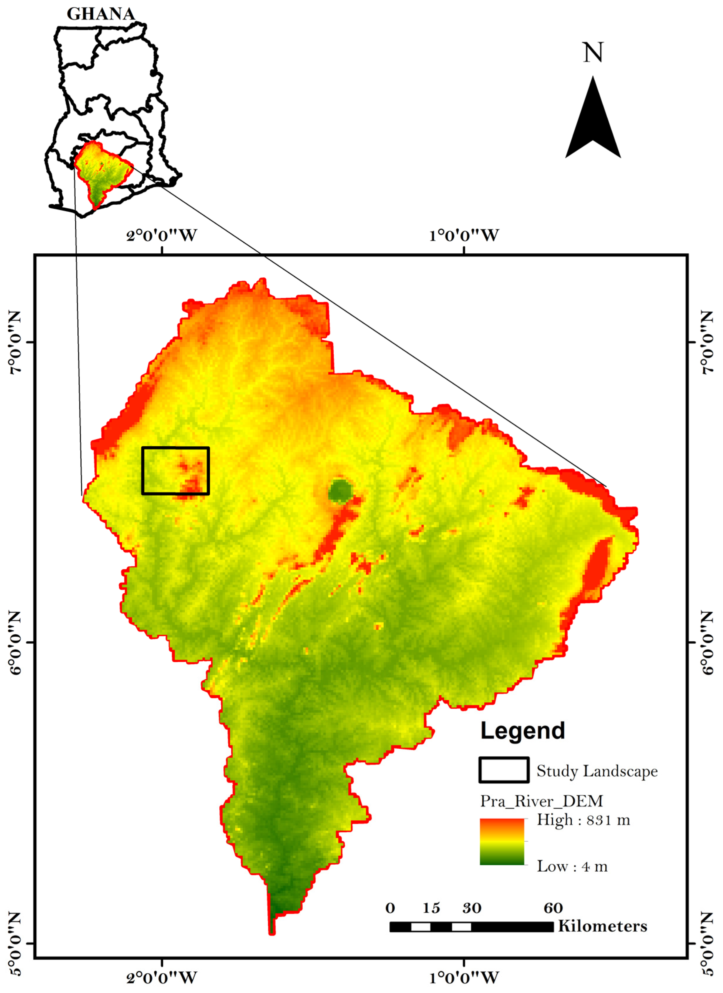
The study landscape is located between Latitude 6°31′00′′ N and 6°37′30′′ N and Longitude 2°4′30′′ W and 1°54′00′′ W. The area, 408.5 km2, was delineated from the Pra River watershed (Figure 1). It covers part of the Atwima Mponua, Atwima, and Amansie West districts. The landscape was selected based on several considerations emanating from the research problem such as the involvement of indigenes in the sector, the extensiveness of the activity, etc. However, the spatial and temporal extent of the study area were delineated considering the poor availability of historical satellite imageries. The area is part of the wet climatic zones that experience a double maxima rainfall (i.e., major and minor rain seasons). The area experiences high rainfall ranging from 1250 mm and 2000 mm. The area records a relative humidity that fluctuates from 70% to 80% throughout the year. Usually, the temperatures of the area fluctuate between 26° and 30° Celsius. Characterised by a relatively flat landscape, the area has an undulating topography and a mean elevation of 450 m above mean sea level (MSL). Forest ochrosols are the predominant soils in this area. These soils are formed from the Tarkwaian sandstones and granitoid as well as metamorphosed phyllites and schists. The vegetation is semi-deciduous, comprising of broad-leaved trees with a height range of about 40 cm or more. However, to some extent land use changes have reduced this closed broadleaved forest to climbers, shrubs/short woody plants and species usually found interspersed within tree remnants [24]. The Water Resource Commission [25] estimates that 60% of the area is covered by agriculture land use, while forest accounts for 30%. Moreover, grassland, human settlement, and other land cover types cover about 10% of the entire watershed. The area has a history of small-scale mining because of its world-class Birimain and Tarkwain rock formations [26,27]. Because of the gold mining activities, most of the settlement is referred to as mining towns.
2.2. Land Cover Monitoring
We approached and mapped the value of the ecosystems degraded due to mining land use along portions of the renowned Pra River Basin of Ghana by using Landsat images. Each image had a spatial resolution of 30 m and a temporal resolution of 16 days. The images were captured with Landsat Thematic Mapper (TM), Enhanced Thematic Mapper (ETM) and Operational Land Imager-Thermal Infrared Sensor (OLI-TIRS) and covered 1986, 2002 and 2016, respectively (Table 1). The original imageries were downloaded from the United States Geological Survey department’s (USGS’) online database (http://glovis.usgs.gov/). The temporal scale was selected to represent the periods such as based year (1986), early-PNDCL period (2002) and late-PNDCL period (2016). The base year represents the year of the promulgation of the PNDC mining laws 218 to legalise the small-scale mining sector. Thus, the study quantified the mining impacts on ecosystems by comparing it to the state of the landscape before and after the activity was legalised.
After the images were downloaded from the USGS’ database, they were processed by using the traditional image processing techniques [28] to extract salient information for the study. The imageries were initially pre-processed to reduce the influence of some commonly embedded defects in satellite images in order that more useful information are extracted. The defects are as a result of atmospheric instability, geographic positioning, sensor shortcomings etc. These defects must be rectified in order to increase the confidence placed in the classified images [29]. First, the radiometric correction was performed on all images using the image calibration algorithms (FLAASH and Band Math) for atmospheric correction in the Environment of Visual Image (ENVI v5.0) software. This was followed by a Hybrid Image Classification Approach (HICA). Here, the pre-processed images were classified, first by separating them into their various band components using the principal component algorithm. The Principal Component Analysis (PCA) combined with visual image interpretation was used as the basis to select training samples. Supervised maximum likelihood classification method was then used to catalogue them into forests, mixed vegetation, built-up areas and mining areas. The forest areas consisted of closed broadleaved wood growth and closed canopied plantations whereas the mixed vegetation describes areas with shrubs (annual and perennial), grasslands, annual crops, harvested crops etc. The developed area covered settlements and roads whereas mining areas described the stagnated turbid waters, bare surfaces closer to mining craters and the mining craters themselves.
Post-classification smoothing and accuracy assessment were also performed. The classified images were smoothened to eliminate the embedded salt and pepper effects by applying the 7 × 7 Kernel majority [30] algorithm in ArcGIS 10.3. The ultimate aim of this paper is to ensure that land management alternatives are selected based on the complete analysis. This required that we put some level of confidence in this environment monitoring analysis. As such, error matrix consisting of a 4 × 4 grid of predicted versus ground truth information was constructed. Known locations of the observed land cover types were selected and mapped as ground truth points. As a precaution, the training sample areas were avoided when selecting the ground truth. Again, ground truth points for each land use type were located evenly and over the entire landscape. This minimised the biases in the confusion matrix. The overall accuracy (i.e., the ratio of correctly classified pixels to all the pixels evaluated) was compared to a discrete multivariate approach to accuracy assessments referred to as Kappa coefficient [31]. The likelihood that the pixels of a land use or a land cover on the ground are predicted as such on the map is indicated by the errors of omission (producer’s accuracy). The error of commission (user’s accuracy) was used as an indicator to detect the likelihood that the pixel designated for a class on the map is truly represented as such on the ground.
The Kappa coefficient (Khat) was calculated using;
where:
Khat is Kappa coefficient; Pa = is the percent correctly classified pixels (actual); Pe is the percent of pixels that were correctly classified by chance (expected); Pp is the percentage of percent correct for perfect classification. Khat > 80% represent strong agreement and good accuracy, 40%–80% is middle, <40% is poor [32,33,34,35].
Following Pyravaud’s formula [36], the study provided the consistent rate of change for each land use type achieved during the image classification phase. The rate of change was computed as follows:
where;
A1 and A2 represent the land cover types in period 1 (t1) and period 2 (t2), respectively.
2.3. Ecosystem Service and the ESV Model
The benefits transfer method combined with biome equivalency approach was used to respectively select and assign value coefficients (VC). The benefits transfer method is a process of using existing values and information from original study sites to estimate ESVs of other similar location in the absence of site-specific value information [21,23]. Thus, each land use type obtained by image classification was related to an equivalent biome [36]. The results of the biome equivalencies and their respective VC are aggregated in Table 2. These values were based on the tropical settings of the original compilations of 1310 values by van der Ploeg and de Groot from local settings worldwide [37]. A total VC of 943.45 US$/ha/year was computed for the forest, and 325.75 US$/ha/year for mixed vegetation. Developed areas were deemed to provide no ecological services values but mining area, with the stagnated waters, could support the water cycling etc. Therefore, we selected the water support value of deserts as an equivalent biome.
The spatial values of the ES were calculated by following the methodological approach expressed in Figure 2. First, area statistics for each land use type was computed for 1986, 2002 and 2016 by using the ArcGIS Version 10.3 software [38]. The area statistic of each land use type was multiplied by their respective coefficients (Equation (3)).
ESV = estimated ecosystem service value, Ai = the area (ha) and VC = the value coefficient (US$ ha−1 year−1) for land cover type ‘i’’. The percentage change of ESV was calculated by using Equation (4) whilst a trade-off matrix was computed for the entire duration of the study.
Sensitivity Analysis
Generally, biomes are not perfect match for land use types. Therefore, there exist uncertainties in the value coefficients used. An additional sensitivity analysis is required to determine the percentage change in ESV for a given percentage change in VC. Referring to the work of Kreuter et al. [21], the coefficient of sensitivity (CS) was calculated bearing in mind the standard economics concept of elasticity. Beforehand, the VCs were adjusted by ±50% of their initial values; thus the total value of ecosystem services estimated using the adjusted VCs is referred to as the adjusted ESVj. The coefficient of sensitivity was estimated as follows:
where:
CS represents the estimated coefficient of sensitivity; ESV refers the total estimated values for the services ecosystems provides. VC is the value coefficients whereas i, j and k, respectively, symbolises the initial, adjusted values and land cover class. To interpret CS, the rule of thumb is that the respective ecosystem service value is elastic if CS > 1 and inelastic if CS < 1 (i.e., inelastic demand). Thus, if the CS < 1, then the ESV estimated is reliable even if there are low accuracies in the VC value of the proxy biomes [21].
3. Results
3.1. Validation Analysis of the Classified Images
The results of post-classification accuracy assessments performed are summarised in Table 3. Indicators such as overall accuracy, user’s accuracies, producer’s accuracies, and Kappa coefficients were used to assess the accuracy level of the land cover classes. The kappa statistic ranged from 0.872 to 0.889. According to Anthony et al. [33], a kappa statistic greater than 60% is substantial or good. Judging from their scale, the classified images are good for further analysis and/or making conclusions about the phenomenon being studied. Similarly, the highest overall accuracy of 91.7% was obtained for 2002 compared to 90.4% and 91.6% in 1986 and 2016, respectively. Additionally, the mining land use type was less accurate in 1986 compared to 2002 and 2016 because of the less conspicuous the mining land use appeared, as well as the issue of spectral un-mixing.
3.2. General Statistics and Spatial Distribution of Land Cover Classes
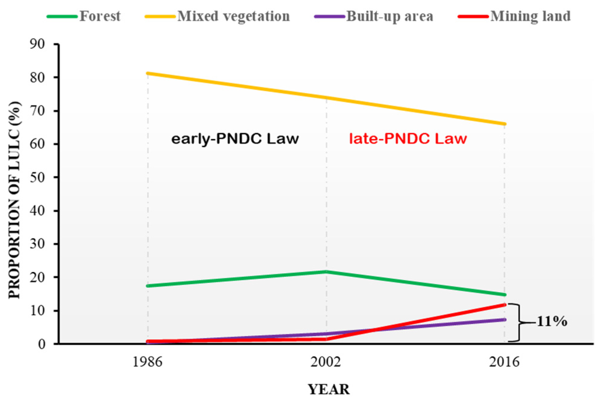
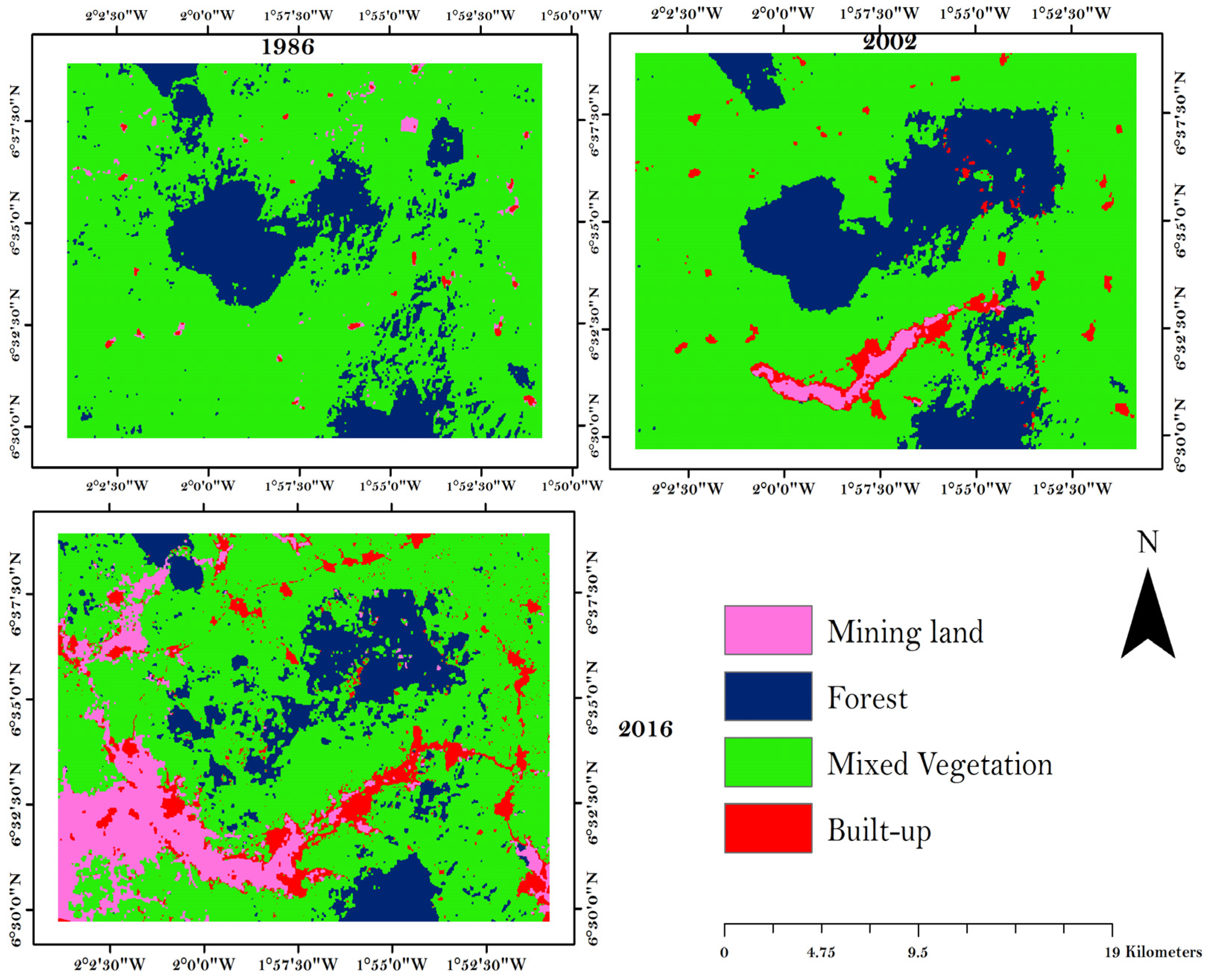
Figure 3 and Figure 4, respectively show the general trends and the spatial distribution of land use and land cover (LUCC) classes of the 1986, 2002 and 2016 images. The area statistics and percent variations in land-uses of the early- and late-PNDCL periods were estimated and summarised in Table 4. A rather irregular but interesting result was observed in the forest cover class. In 1986, the forests occupied 7147.8 hectares, which represents 17.5% of the total study area. By 2002, the forest cover increased to 8886.4 hectares (21.8%) at 1.7% per annum but declined to 6053.4 hectares, which represented 14.8% of the total area in 2016, at 2.0% per annum. The mixed vegetation, which was the largest cover class at 33161.4 hectares and represented 81.2% of the total area in 1986, decreased significantly at 0.6% per annum to 26989.2 hectares (66.1%) in 2016. Moreover, the built-up and mining areas increased substantially throughout the study periods. Thus, the 354.9 hectares of mining land in 1986, which represented 0.9% of the total area, increased significantly to 4804.1 hectares (11.8%) in 2016 at 41.8% per annum. A significantly higher growth rate at 47.5% per annum was observed in the late-PNDCL period (2002–2016) compared to the early-PNDCL period (1986–2002), which grew at 4.1% per annum. Similarly, the built-up area increased steadily from 189.6 hectares, which represents 0.5% of the total area in 1986, at 49.5% per annum to 3007.17 hectares (7.4%) in 2016.
Spatially, the built-up area and the mixed vegetation cover patches were nearly evenly distributed within the study landscape in 1986. However, the forest cover type was concentrated in the central parts. Mined lands were initially found in the north-eastern (NE) part of the study landscape but in 2002, the mining activities were more profound in the southern parts. In 2016, the mining areas were mostly found in the western part of the landscape. The patches representing mining land-use were widely extended and new patches emerged from 1986 to 2016. In fact, the extension of mining patches and the formation of patches in new locations clearly show the migratory pattern of the small-scale mining activity.
3.3. Land Use Change Trajectory Matrix from 1986 to 2002 to 2016
The land cover types of the study landscape have changed markedly due to the interchanges with land uses. The changes are quantified in terms of area coverage measured in hectares and percentages (%). For the purposes of this study, the results of the transition trajectory were grouped into trade-off and unchanged areas. Trade-off areas were further categorised into positive (recovered) and negative (degraded) trade-offs. By 2002, a total 6174.36 hectares, which accounted for 15.1% of the total area, experienced trade-offs between land uses whereas 34,679.52 hectares, which represents 84.9% of the total area, remained unchanged. The mining activities had expanded to cover a relatively smaller area of 3.87 hectares of forest compared to the mixed vegetated areas, which lost about 552.24 hectares to the small-scale mining activities (Table 5). Overall, the mining activities had negatively affected about 9.0% of the 6174.36 hectares of trade-off areas of the study landscape. Again, from the 354.9 hectares of mining lands observed in 1986, about 63.27 and 193.86 hectares were recovered into the forest and mixed vegetation, which represents about 4.2% of the total trade-offs land uses.
In the late-PNDCL period, the land use interchanges (gain or loss) occurred on 11,486.2 hectares, which represented 28.1% of the total area whereas 29,367.7 hectares, representing 71.9% of the total area, remained unchanged. The small-scale mining activities degraded 83.67 hectares of forest and 4029.21 hectares of mixed vegetation over the sixteen-year period. Overall, the mining activities were the reasons for about 38.2% of the land use changes within the study landscape. Thus, the mining activity degraded approximately 38% of other ecosystems, including forest and mixed vegetation. However, of the 558.2 hectares of mining land patches that existed in 2002, only about 0.36 and 76.50 hectares of the forest and mixed vegetation ecosystems were recovered, respectively. Thus, about less than 0.01% of the interchanged areas in 2016. By 2002, no built-up land was lost to mining activities but by 2016, about 273.2 hectares of the built-up area lost to mining. This may be due to the incorrectly separated pixel values between the mining and the built-up areas. More robust image classification approaches such as the object-based approach to image classification may be employed to ascertain the pixel separability issues between built-up areas and mining lands in further studies.
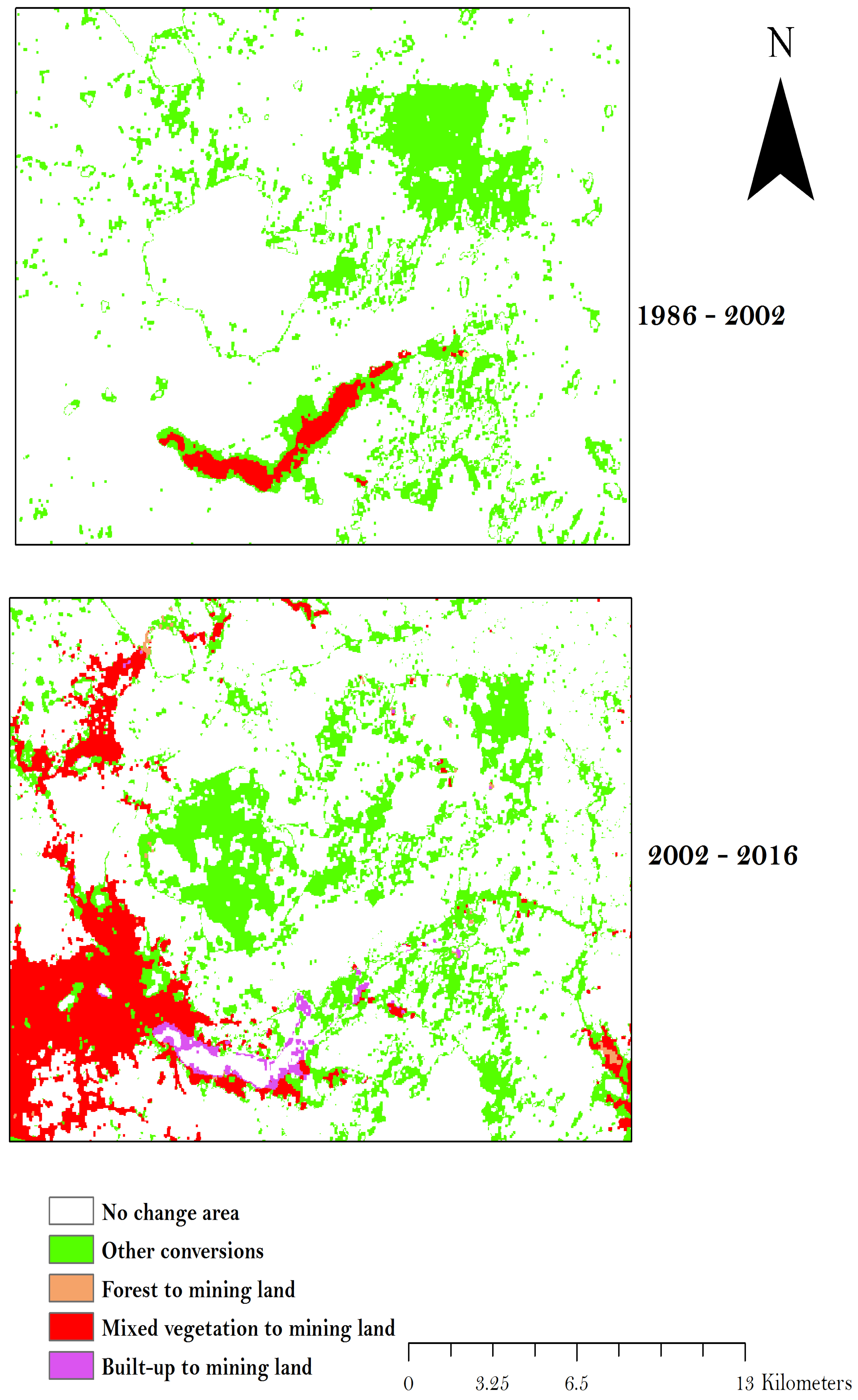
Figure 5 shows the spatial trajectory of land cover changes in the study landscape. In the figure, a particular emphasis is placed on the mining land conversions. The most significant conversion trajectory was from mixed vegetation to mining land use, shown in red colour (online version). Thus, a total of 552.24 hectares and 4029.21 hectares of mixed vegetated land was lost to mining activities from 1986 to 2002 and 2002 to 2016, respectively. The land-use change matrices are presented in Table 5 and Table 6.
3.4. General Variation of ESV amongst Land Use Types
The value of the services (ESVs) each land cover, herein referred to as ecosystem, provides, were estimated, grouped under multi-temporal scale, and summarised in Table 7. Because of the non-linearity in the some of the observed trends, the forest cover type and the total ESV, it was vital to establish the ESV yearly. In this regard, the Pyravaud’s formula helped to reduce the inconsistencies.
The study landscape provided a total ecosystem service of 17.69 million US$ in 1986 of which forest cover contributed 6.89 million US$ (38.9%) whereas mixed vegetation provided 10.80 million US$ (61.1%). By 2002, the ESV of the entire landscape had increased at 0.3% per annum to 18.40 million US$. These increments were because of the cushioning effect of the increased services of forest ecosystem at 1.7% per annum, which overwhelmed the decreasing impact of the mixed vegetation at 0.6% per annum. Even though the built-up and mined lands had increased significantly in size to 3.0% and 1.4%, respectively (Table 7), the effects were not considerable because of the neutralising influence of the increased forest and the subsequent increase in ESV. Additionally, by 2016, the ESV had decreased to 14.63 million US$ at 1.3% per annum. This decrease in the total ESV is associated with the decrease in the ESV of mixed vegetation at 0.7% per annum and forest at 2.0% per annum, respectively. Considering the entire period for this evaluation (1986–2016), a net loss of ESV of 3.06 million US$ was recorded, representing 17.3% of the total ESV observed in 1986. The observed decrease in ESV for this period is attributed to the net decrease in the services the forests at 2.01 million US$ and mixed vegetation at 1.06 million US$. Figure 6 shows the spatial representation of the ESV of the studied landscape. In 1986, larger proportion (82%) of the landscape provided more ESV per hectare than the average for the entire landscape (i.e. US$ 490 per hectare). Similarly, the ESV per hectare of larger proportion (85%) of the study area are more than the average of US$ 560 per hectare recorded in 2002. A relatively smaller proportion (57%) of the 2016 ESV image had values that were more than US$ 351 per hectare.
3.5. Impacts of Small-Scale Gold Mining on Ecosystem Services Delivery
Our study described the impacts of small-scale gold mining on ES delivery as the “forgone” ESVs of the respective ecosystems. Using the size of the land cover type that is converted (traded-off) to the mining area and the associated VC, the study has estimated the value of the ecosystems forgone to make available small-scale gold mining. The ESV estimated for each forgone ecosystem are summarised in Table 8. From 1986 to 2002, the land cover types of the study areas collectively lost 0.18 million US$ to small-scale mining activities; 0.004 million US$ from forest and 0.180 million US$ from mixed vegetation. The total forgone ESV of 1.39 million US$ achieved for the late-PNDCL period (2002–2016) was approximately eight times higher than the value estimated for 1986–2002. Likewise, 0.08 million US$ and 1.31 million US$ were lost from the forest and mixed vegetation, respectively, to pave way for the mining activities.
The biomes being ecosystem proxies and the fact that the VC were borrowed through benefits transfer method makes the ESV estimates open to uncertainties. As such, the researcher showed how a 1% change in ESV would affect the ESV estimates. As recommended by Kreuter et al. [21], all VCs were adjusted by 50% in order to provide a range of ESV values for each land use category. The results achieved by varying value coefficients (VCs) and their effects on the forgone estimate of ESV are summarised in Table 8. As a rule, all CS estimates were compared to one (1). Though the estimated CS of forest cover type increased from 0.016 to 0.058 while the CS of mixed vegetation decreased from 0.978 to 0.942, the ESV estimates are robust since the CS are more than one (1). The results indicate that ESV for all land use categories are inelastic, and thus making the estimated total ESV inelastic.
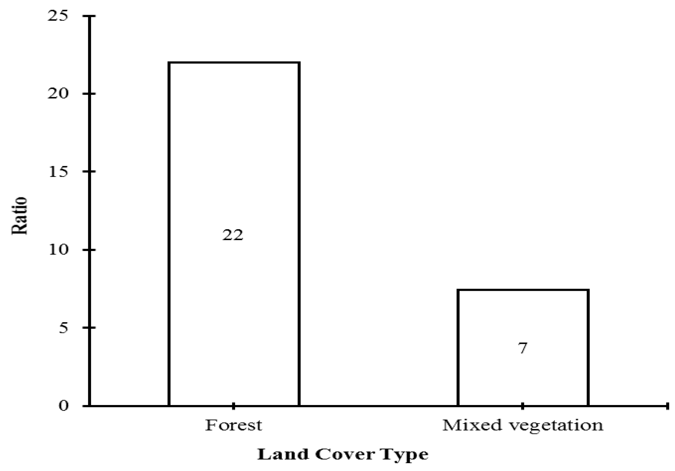
The net decline in forest services and mixed vegetation were also compared. The ratio of the forgone values in the early- law to the late- law periods are shown in Figure 7. Even though the area of change in the forested land is relatively small, their decline for small-scale mining, in monetary term, is considerable during the 1986–2002 at approximately 22 folds compared to the late-PNDCL period of 2002 to 2016. Likewise and in the same temporal trajectory, the mining activities decreased the mixed vegetation by seven (7) folds.
Comparing the “forgone” ESV of mining to the “money realised” from the activity is essential for a deeper understanding of the losses the activities (small-scale mining) incur on the ecosystem. Table 9 provides a summary of the comparison made. The small-scale miners realise an amount of US$ 11,517.00 per hectare per annum from the sale of gold. The value of ecosystems degraded differs by US$ 86,476.28 per hectare per annum.
4. Discussion
4.1. The Influence of Land Use Dynamics on Ecosystem Service Delivery
The spatial and temporal dynamics of land uses are important to establish. In this study, the impacts of land-use are measured by estimating the magnitude of the decline in the services their ecosystems deliver for the well-being of humans. Remotely-sensed datasets of three decades were obtained and analysed to provide information on the ecosystem services values (ESVs) degraded due small-scale gold mining land-use. By using the Constanza’s ESV model [4] and some borrowed value coefficients (VCs), the ESV of a mining landscape were estimated by multiplying the area (ha) of land use types by the respective VC (US$/ha/year). As discussed earlier, the ESV estimates are subject to uncertainties and variations, due to factors such as non-linearity of the dynamics of ecosystems, scale, double counting, quality of classified images etc. [40,41,42]. The robustness of the estimated CS combined with the fact that accurate coefficients are could be less critical for time series than for cross-sectional analyses, because value coefficients tend to affect estimates of directional change less than estimates of ecosystem values at specific points in time [43,44], makes the ESV estimation was robust in spite of uncertainties on the value coefficients.
Considering the landscape in its entirety, total ESV in the base year of 1986 was 17.69 million US$, but increased by 0.71 million US$ at 0.3% per year to 18.40 million US$ in the early-law period, and subsequently decreased considerably by 3.77 million US$ at a rate of 1.3% per year to 14.63 million US$ in the late-PNDCL period. It is imperative to report that the interchanges among these land use types translated into the decline or rise in ecosystem functions. A transition from one land use type to another is associated with an increase or a decrease in ESV. Therefore, the appreciation in the total ESV could be a result of the increased size and a subsequent increase in the ecological functions of forest and mixed vegetation from 1986 to 2002. The enormous reforestation that occurred in this period could explain the rise in the ESV of the study landscape. This implies that reforestation is a good way to recover and/or restore the productive capacities of the landscape. This, however, may be associated with the improved forest protection laws and follow-up monitoring schemes. As such, most of the mixed vegetation around the forests were abandoned while they reforest. Wang et al. [45] also observed the cushioning impact of increased forest cover on the total ESV of Ningxia of China. Moreover, the forest becoming patchy due to fragmentation and the influx of other land use types into the forest areas caused deforestation and decreased the overall services the landscape provided in 2016. The current estimates of the land use/land cover along the Pra River watershed Ghana also reveals the deforestation for mining, farming, and settlement development [25]. The observed fluctuation (i.e., rise and fall) in the ESV signal that when drivers of change are put to check, sustainability goals can be achieved.
4.2. The “Forgone Value” of Ecosystem Services Due to Mining
The impacts of mining land use on the ecological systems were measured by determining the ESVs of the land use types that were converted to mining land use. Here, the ESV of the declined land use type was described as “forgone” values. Two distinctive periods, which includes early- and late-PNDCL, were compared. We have to admit that a myriad of factors cause and/or accelerate the changes in the land use and land cover of a particular geographical setting. These factors may include but not limited to policies, human land use (agriculture expansion, mining, roads etc.), population, natural factors etc. [46,47]. In fact, most of these factors could explain the dynamics of the other land use types observed in this study. Nevertheless, our analysis emphasised policy effects on the mining land use expansion. Literature has revealed that GoG legalised the small-scale mining sector to improve the economy of the country [48]. The use of land in this regard, however, aligns with the fact that humans use land in a certain way to suit a particular purpose and as such degrades the ecological resources [49]. However, decisions involving tradeoffs involve valuation [50]. The GoG has prioritised the needs of the people to the ecological system. This does not imply that such decisions are “bad”. However, the inability of these small-scale mining laws to capture the reality of the sector’s activities has made this ecological service trade-off to become considerable [51].
The results have indicated a similar trend and have demonstrated that land use policy is one of the key factors that can contribute significantly to the dynamics of the mining landscape. In this study, about 1.37 million US$ of the services of other ecosystems (forest and mixed vegetation) was traded off for mining activities, which represents 36.3% of the net decline in the ESV from 2002 to 2016. This signals the profound implications of mining land use during the late-PNDC mining laws period compared to the early-PNDCL period, which accounted for about 8.4% of the total net decline. Overall, the mining activities have caused the decline of approximately 47% of the total ESVs of the landscape over the 30 years period of study. The transition from forest to mining was associated with a significant drop in their ecosystem service values. Due to the considerable magnitude of the forest VC, a minimal drop in the expanse is associated with a considerable decrease of the total ESV. The results are attributed to the significant roles the forests play in human well-being such as climate regulations, food production, water and air purification, raw materials etc. This, as well, signals that the enormous fragmentation of the forest correlates with ecosystem services decline. Consequently, a higher decline in ESV is expected when there is a considerable decline in forested land. The results did not come as surprise since DeFries et al. [2] reports that whenever a land use decision is made, there are often some unintended consequences, including feedbacks to climate, altered flows of freshwater, changes in disease vectors, and reductions in biodiversity. In fact, the forgone ESV from this study was lesser than the estimated 8.70 million US$ from Boshie et al. [52]. This may be due to the scale of their study (i.e., a higher value is expected at a district scale compared to a landscape scale).
5. Conclusions
Ghana’s economic development relies largely on gold industry, but the ecological cost is very high particularly from the small-scale sector. The study at hand gives an account of the ecological pressures from the small-scale gold mining sectors. These pressures were measured by considering the ecosystems (land cover types), which are affected by the small-scale mining. Thus, the extent and the magnitude of the ESV associated with the land cover that was stripped to make available the small-scale gold mining, as well as the sustainability of two production systems were estimated. Historical data covering a period of 30 years (1986–2016) was used in this study. In general, the land use types of the study landscape were distinctively dynamic from 1986 to 2002 to 2016. The expanse of mining land use increased from 0.9% in 1986 to 11.8% in 2016. However, the annual growth rate during the early-PNDCL of 4.1% was significantly lower compared to the late-PNDCL of 47.5%. The study also estimated and compared the trade-off regions to the unchanged regions by using a per-pixel change trajectory matrix. A considerable percentage of the trade-off areas was associated with small-scale gold mining. Comparatively, greater mining-related land use dynamics, which include the expansion of mining land use patches and the formation of new ones, were observed during the late-PNDCL period (2002–2016; 36.3%) compared to the early-PNDCL period (1986–2002; 8.4%). In monetary term, the small-scale gold mining was responsible for about 1.43 million US$ of the 3.06 million US$ net decline of the ecological services of the landscape from 1986 to 2016. The mining activities encroaching forest and mixed vegetation accounted for 0.06 and 1.37 million US$ of the net decline of the ESV of the study area. The study delved only into the spatiotemporal dimension the mining land use change of the study landscape, but when supplemented with previous scholarly works, it appears the laws are enacted but fail to check and sanction defaulters. The study would contribute to better understanding of the variation in ESVs, their dynamics, and the evolution of small-scale mining. It has provided the scientific basis for informing land management and environmental protection policies.
Acknowledgments
This work was supported by the National Science and Technology Major Project of the Ministry of Science and Technology of China (2017YFC0505703), Funds for International Cooperation and Exchanges of the National Natural Science Foundation of China (51661125010) and National Natural Science Foundation of China (41371521). E.F. Asamoah acknowledges Tamara Mwanza for her contribution towards the preparation of the manuscript.
Author Contributions
L.X. Zhang, E.F. Asamoah and G. Liu conceived and designed the experiments; Asamoah performed the experiments; E.F. Asamoah and E. Rukundo analysed the data; N. Owusu-Prempeh contributed reagents/materials/analysis tools; E.F. Asamoah wrote the paper.
Conflicts of Interest
The authors declare no conflict of interest.
References
- Millennium Ecosystem Assessment (MA). Millennium Ecosystem Assessment: Living Beyond Our Means-Natural Assets and Human Well-Being; World Resources Institute: Washington, DC, USA, 2005. [Google Scholar]
- DeFries, R.S.; Foley, J.A.; Asner, G.P. Land-use choices: Balancing human needs and ecosystem function. Front. Ecol. Environ. 2004, 2, 249–257. [Google Scholar] [CrossRef]
- The World Bank. Sustainable Land Management: Challenges, Opportunities, and Trade-offs; The World Bank: Washington, DC, USA, 2006. [Google Scholar]
- Costanza, R.; d’Arge, R.; de Groot, R.; Farberk, S.; Grasso, M.; Hannon, B.; Limburg, K.; Naeem, S.; O’Neill, R.V.; Paruelo, J.; et al. The value of the world’s ecosystem services and natural capital. Nature 1997, 387, 253–260. [Google Scholar] [CrossRef]
- Von Wieser, F. Social Economics; Adelphi: New York, NY, USA, 1927. [Google Scholar]
- PwC Analysis. The Direct Economic Impact of Gold. 2013. Available online: https://www.pwc.com/gx/en/mining/publications/assets/pwc-the-direct-economic-impact-of-gold.pdf (accessed on 19 February 2017).
- Hilson, G. The environmental impact of small-scale mining in Ghana: Identifying problems and possible solutions. Geogr. J. 2002, 168, 57–72. [Google Scholar] [CrossRef]
- Cooke, J.A.; Johnson, M.S. Ecological restoration of land with particular reference to the mining of metals and industrial minerals: A review of theory and practice. Environ. Rev. 2002, 10, 41–71. [Google Scholar] [CrossRef]
- Hammond, D.S.; Gond, V.; de Thoisy, B.; Forget, P.-M.; DeDijn, B.P.E. Causes and consequences of a tropical forest gold rush in the Guiana Shield, South America. AMBIO 2007, 36, 661–670. [Google Scholar] [CrossRef]
- Schueler, V.; Kuemmerle, T.; Schröder, H. Impacts of surface gold mining on land use systems in Western Ghana. AMBIO 2011, 40, 528–539. [Google Scholar] [CrossRef] [PubMed]
- Hentschel, T.; Hruschka, F.; Priester, M. Global Report on Artisanal and Small-Scale Mining: Challenges and Opportunities; International Institute for Environment and Development (IIED) and WBCSD Publishing: London, UK, 2003. [Google Scholar]
- Al-Hassan, S.; Amoako, R. Environmental and security aspects of contemporary small-scale mining in Ghana. In Proceedings of the Third UMaT Biennial International Mining and Mineral Conference, Tarkwa, Ghana, 30 July–2 August 2014; pp. 146–151. [Google Scholar]
- Kessey, K.D.; Arko, B. Small Scale Gold Mining and Environmental Degradation, in Ghana: Issues of Mining Policy Implementation and Challenges. J. Stud. Soc. Sci. 2013, 5, 12–30. [Google Scholar]
- Duncan, E.E.; Kuma, J.S.; Primpong, S. Open Pit Mining and Land Use Changes: An Example from Bogosu-Prestea Area, Southwest Ghana. EJISDC 2009, 36, 1–10. [Google Scholar]
- Basommi, L.P.; Guan, Q.; Cheng, D.; Singh, S.K. Dynamics of land use change in a mining area: A case study of Nadowli District, Ghana. J. Mt. Sci. 2016, 13, 633–642. [Google Scholar] [CrossRef]
- Basommi, P.L.; Guan, Q.; Cheng, D. Exploring Land use and Land cover change in the mining areas of Wa East District, Ghana using Satellite Imagery. Open Geosci. 2015, 7, 618–626. [Google Scholar] [CrossRef]
- Snapir, B.; Simms, D.M.; Waine, T.W. Mapping the expansion of galamsey gold mines in the cocoa growing area of Ghana using optical remote sensing. Int. J. Appl. Earth Obs. Geoinf. 2017, 58, 225–233. [Google Scholar] [CrossRef]
- Kindu, M.; Schneider, T.; Teketay, D.; Knoke, T. Changes of ecosystem service values in response to land use/land cover dynamics in Munessa-Shashemene landscape of the Ethiopian highlands. Sci. Total Environ. 2016, 547, 137–147. [Google Scholar] [CrossRef] [PubMed]
- Scholes, R.J. Chapter IV: Ecosystem Services: Issues of Scale and Trade-Offs. In The Princeton Guide to Ecology; Levin, S.A., Carpenter, S.R., Godfray, H.C.J., Kinzig, A.P., Loreau, M., Losos, J.B., Walker, B., Wilcove, D.S., Morris, C.G., Eds.; Princeton University Press: Princeton, NJ, USA, 2009. [Google Scholar]
- Payne, C.R.; Sand, P.H. Gulf War Reparation and the UN Compensation: Environmental Liability; Oxford University Press: New York, NY, USA, 2011. [Google Scholar]
- Kreuter, U.P.; Harris, H.G.; Matlock, M.D.; Lacey, R.E. Change in ecosystem service values in the San Antonio area, Texas. Ecol. Econ. 2001, 39, 333–346. [Google Scholar] [CrossRef]
- Wang, Z.; Zhang, B.; Zhang, S.; Li, X.; Liu, D.; Song, K.; Li, J.; Li, F.; Duan, H. Changes of land use and of ecosystem service values in Sanjiang Plain, Northeast China. Environ. Monit. Assess. 2006, 112, 69–91. [Google Scholar] [CrossRef] [PubMed]
- Kubiszewski, I.; Costanza, R.; Dorji, L.; Thoennes, P.; Tshering, K. An initial estimate of the value of ecosystem services in Bhutan. Ecosyst. Serv. 2013, 3, 11–21. [Google Scholar] [CrossRef]
- Dickson, K.B.; Benneh, G. A New Geography of Ghana; Longman: London, UK, 1995; pp. 21–33. [Google Scholar]
- The Water Resources Commission. PRA RIVER BASIN—Integrated Water Resources Management Plan. 2012. Available online: http://doc.wrc-gh.org/pdf/Pra%20Basin%20IWRM%20Plan.pdf (accessed on 9 April 2017).
- Dumett, R.E. El Dorado in West Africa; Ohio University Press: Athens, OH, USA, 1998; pp. 1–396. [Google Scholar]
- Donkor, A.K.; Bonzongo, J.C.; Nartey, V.K.; Adotey, D.K. Mercury in different environmental compartments of the Pra River Basin, Ghana. Sci. Total Environ. 2006, 368, 164–176. [Google Scholar] [CrossRef] [PubMed]
- Jensen, J. Introduction Digital Image Processing: A Remote Sensing Perspective, 2nd ed.; Prentice Hall: New York, NY, USA, 1996. [Google Scholar]
- Badreldin, N.; Sanchez-Azofeifa, A. Estimating Forest Biomass Dynamics by Integrating Multi-Temporal Landsat Satellite Images with Ground and Airborne LiDAR Data in the Coal Valley Mine, Alberta, Canada. Remote Sens. 2015, 7, 2832–2849. [Google Scholar] [CrossRef]
- Kumar, M. Digital Image Processing, Photogrammetry and Remote Sensing Division of Indian Institute of Remote Sensing, Dehra Du. Available online: http://www.wamis.org/agm/pubs/agm8/Paper-5.pdf (accessed on 1 September 2017).
- Congalton, R.G.; Green, K. Assessing the Accuracy of Remotely Sensed Data: Principles and Practices, 2nd ed.; CRC Press Inc.: London, UK, 2009. [Google Scholar]
- Landis, J.R.; Koch, G.G. The measurement of observer agreement for categorical data. Biometrics 1977, 33, 159–174. [Google Scholar] [CrossRef] [PubMed]
- Anthony, J.; Viera, M.D.; Joanne, M.G. Understanding Inter observer Agreement: The Kappa Statistic. Fam. Med. 2005, 37, 360–363. [Google Scholar]
- Saraux, A.; Tobón, G.J.; Benhamou, M.; Devauchelle-Pensec, V.; Dougados, M.; Mariette, X.; Berenbaum, F.; Chiocchia, G.; Rat, A.C.; Schaeverbeke, T. Potential classification criteria for rheumatoid arthritis after two years: Results from a French multi center cohort. Arthritis Care Res. 2013, 65, 1227–1234. [Google Scholar] [CrossRef] [PubMed]
- Liu, C.C. Analysis and Applications of Remote Sensing Imagery (PPT Slide). 2015. Available online: http://slideplayer.com/slide/5332471/ (accessed on 2 September 2017).
- Puyravaud, J.-P. Standardizing the Calculation of the Annual Rate of Deforestation. For. Ecol. Manag. 2003, 177, 593–596. [Google Scholar] [CrossRef]
- Van der Ploeg, S.; de Groot, D. The TEEB Valuation Database—A Searchable Database of 1310 Estimates of Monetary Values of Ecosystem Services; Foundation for Sustainable Development: Wageningen, The Netherlands, 2010. [Google Scholar]
- Environmental Systems Research Institute (ESRI). ArcGIS Desktop: Release 10.3 Redlands; Environmental Systems Research Institute: Redlands, CA, USA, 2014. [Google Scholar]
- Asamoah, E.F. The Ecological Burden of Gold Mining in Ghana: A Remote Sensing Based Monitoring of a Mining Landscape and an Emergy Sustainability Synthesis of Two Small-Scale Production Systems. Master’s Thesis, Beijing Normal University, Beijing, China, 2017. [Google Scholar]
- Limburg, K.E.; O’ Neill, R.V.; Costanza, R.; Farber, S. Complex systems and valuation. Ecol. Econ. 2002, 41, 409–420. [Google Scholar] [CrossRef]
- Konarska, K.M.; Sutton, P.C.; Castellon, M. Evaluating scale dependence of ecosystem service valuation: A comparison of NOAA-AVHRR and Landsat TM datasets. Ecol. Econ. 2002, 41, 491–507. [Google Scholar] [CrossRef]
- Turner, R.K.; Paavola, J.; Cooper, P.; Farber, S.; Jessamy, V.; Georgiou, S. Valuing nature: Lessons learned and future research directions. Ecol. Econ. 2003, 46, 493–510. [Google Scholar] [CrossRef]
- Hein, L.; van Koppen, K.; de Groot, R.S.; van Ierland, E.C. Spatial scales, stakeholders and the valuation of ecosystem services. Ecol. Econ. 2006, 57, 209–228. [Google Scholar] [CrossRef]
- Maes, J.; Egoh, B.; Willemen, L.; Liquete, C.; Vihervaara, P.; Schägner, J.P.; Grizzetti, B.; Drakou, E.G.; La Notte, A.; Zulian, G.; et al. Mapping ecosystem services for policy support and decision making in the European Union. Ecosyst. Serv. 2012, 1, 31–39. [Google Scholar] [CrossRef]
- Wang, Y.; Gao, J.; Wang, J.; Qiu, J.; Bond-Lamberty, B. Value assessment of ecosystem services in nature reserves in Ningxia, China: A response to ecological restoration. PLoS ONE 2014, 9, e89174. [Google Scholar] [CrossRef] [PubMed]
- Nurwanda, A.; Zain, A.F.M.; Rustiadi, E. Analysis of land cover changes and landscape fragmentation in Batanghari Regency, Jambi Province. Procedia Soc. Behav. Sci. 2016, 227, 87–94. [Google Scholar] [CrossRef]
- Zhan, J.; Wu, F.; Li, Z.; Lin, Y.; Shi, C. Land degradation induced by climate and land-use change in the North China Plain. In Impacts of Land-use Change on Ecosystem Services; Zhan, J., Ed.; Springer Geography; Springer-Verlag GmbH: Berlin, Germany, 2015. [Google Scholar] [CrossRef]
- Hilson, G. Small-scale mining and its socio-economic impact in developing countries. Nat. Resour. Forum 2002, 26, 3–13. [Google Scholar] [CrossRef]
- Di Gregorio, A. Land cover vs. land use. In Proceedings of the Global Land Use Data Workshop, Vienna, Austria, 22–23 May 2008. [Google Scholar]
- Costanza, R.; Kubiszewski, I.; Ervin, D.; Bluffstone, R.; Boyd, J.; Brown, D.; Chang, H.; Dujon, V.; Granek, E.; Polasky, S.; et al. Valuing ecological systems and services. F1000 Biol. Rep. 2011, 3. [Google Scholar] [CrossRef] [PubMed]
- Teschner, B.A. Small-scale mining in Ghana: The government and the galamsey. Resour. Policy 2012, 37, 308–314. [Google Scholar] [CrossRef]
- Boshie, G.; Dzanku, F.M.; Akabzaa, T. Open Cast Mining and Environmental Degradation Cost in Ghana; Institute of Statistical, Social, and Economic Research (ISSER): Accra, Ghara, 2008. [Google Scholar]
Figure 1.
A map of Ghana showing the geographical location of study landscape.

Figure 2.
Flowchart of image processing procedure and the estimation of the spatial Ecosystem Service Value (ESV).
Figure 2.
Flowchart of image processing procedure and the estimation of the spatial Ecosystem Service Value (ESV).
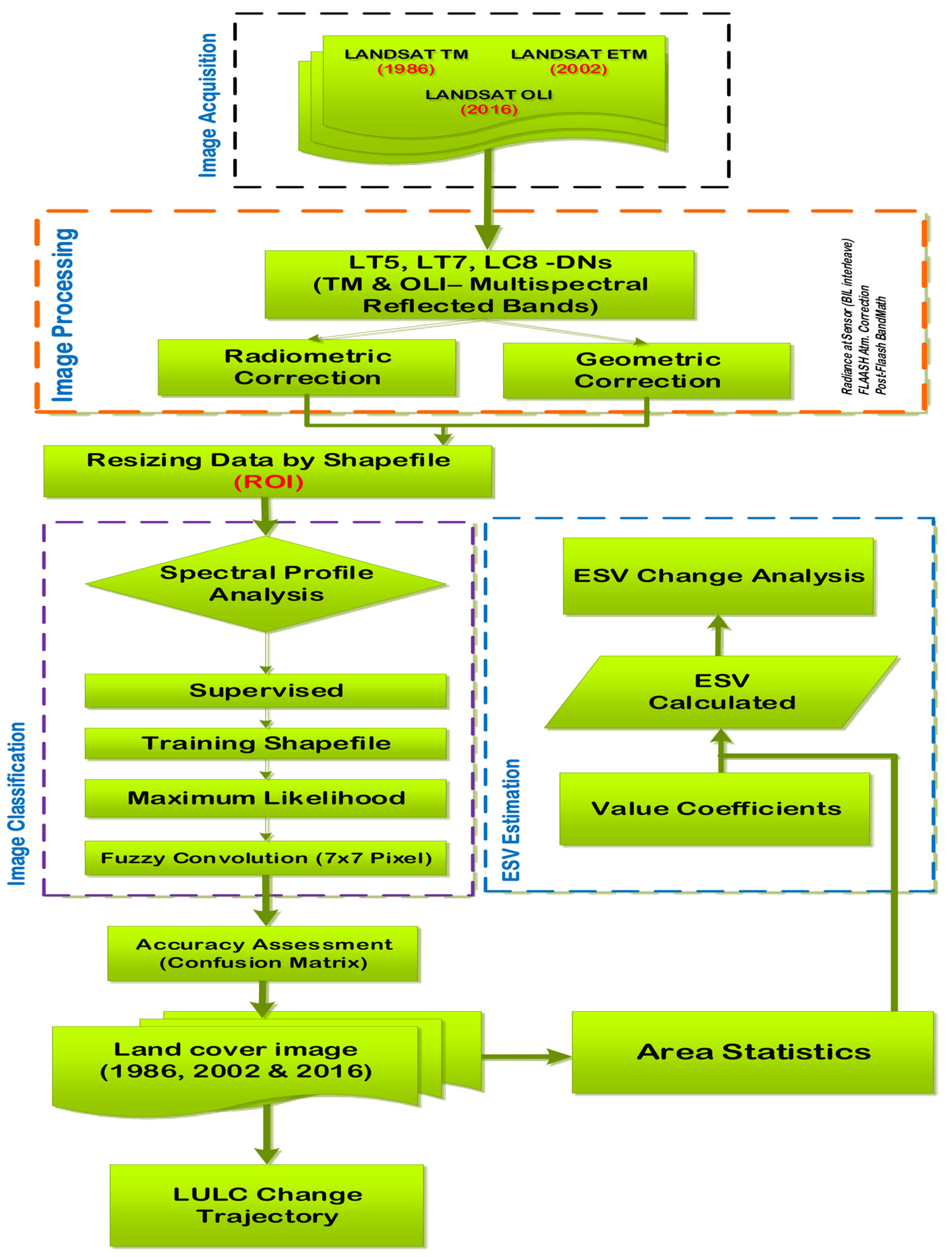
Figure 3.
Trends in land-use grouped under early- and late-PNDC law periods.

Figure 4.
Spatial distribution of land use types in 1986, 2002 and 2016.

Figure 5.
Spatial representation of the land-use change trajectory achieved for the mining land use conversions.
Figure 5.
Spatial representation of the land-use change trajectory achieved for the mining land use conversions.

Figure 6.
Spatial distribution of ecosystem services across the study landscape.
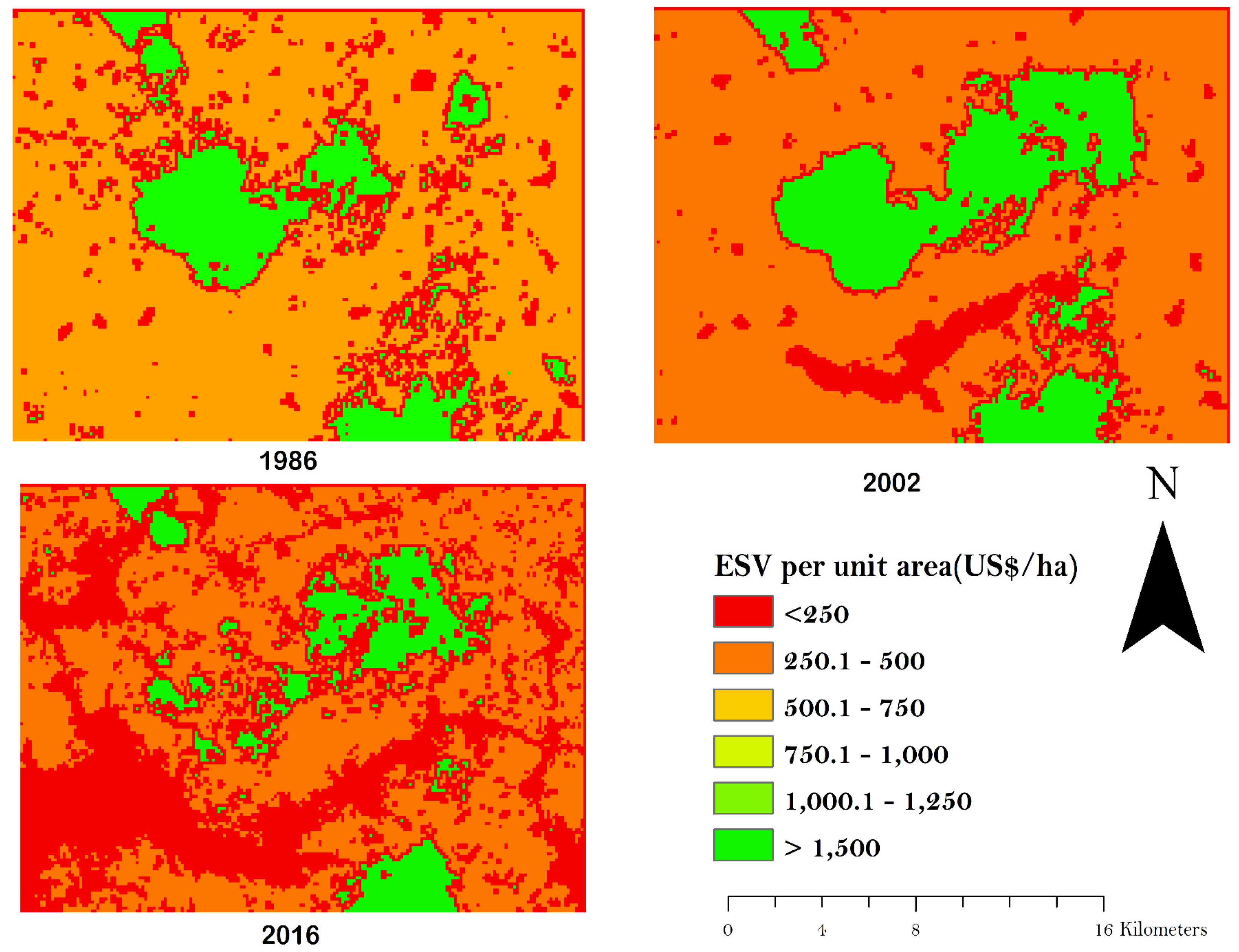
Figure 7.
The ratio of the forgone Ecosystem Service Values (FESVs) observed in the early- Provisional National Defense Council Law (PNDCL) to the late-PNDCL periods, grouped under land uses.
Figure 7.
The ratio of the forgone Ecosystem Service Values (FESVs) observed in the early- Provisional National Defense Council Law (PNDCL) to the late-PNDCL periods, grouped under land uses.


Table 1.
Image data used for the study.
| Product | Date | Resolution (m) | Temporal (Days) |
|---|---|---|---|
| Landsat 5 TM | 29 December 1986 | 30 | 16 |
| Landsat 7 ETM | 15 January 2002 | 30 | 16 |
| Landsat 8 OLI-TIRS | 23 January 2016 | 30 | 16 |
Table 2.
The equivalent biomes per land use type and their respective value coefficients.
| Land Cover Type | Equivalent Biome | ESV (US$/ha/Year) |
|---|---|---|
| Mining area | Semi-desert | 0.38 |
| Forest | Tropical forest | 963.45 |
| Developed area | Urban | 0.00 |
| Mixed vegetation | Multiple ecosystems | 325.75 |
Table 3.
Accuracies achieved for the classified Landsat images.
| Year | Overall Accuracy (%) | Mining Land Use | Kappa Coef. | |
|---|---|---|---|---|
| User’s Accuracy (%) | Producer’s Accuracy (%) | |||
| 1986 | 90.4 | 87.2 | 91.1 | 0.872 |
| 2002 | 91.7 | 75.8 | 93.8 | 0.889 |
| 2016 | 91.6 | 90.5 | 86.9 | 0.886 |
Table 4.
Area statistics of the land use types.
| Year | Forest | Mixed Vegetation | Built-up Area | Mining Land | ||
|---|---|---|---|---|---|---|
| Base Year | 1986 | Area (ha) % | 7147.8 | 33,161.4 | 189.6 | 354.9 |
| 17.5 | 81.2 | 0.5 | 0.9 | |||
| Early-PNDCL | 2002 | Area (ha) % | 8886.4 | 30,199.3 | 1210.0 | 558.2 |
| 21.8 | 73.9 | 3.0 | 1.4 | |||
| Late-PNDCL | 2016 | Area (ha) % | 6053.4 | 26,989.2 | 3007.2 | 4804.1 |
| 14.8 | 66.1 | 7.4 | 11.8 | |||
| Rate | 1986–2002 | % | 1.7 | −0.6 | 38.4 | 4.1 |
| 2002–2016 | % | −2.0 | −0.7 | 9.3 | 47.5 | |
| 1986–2016 | % | −0.6 | −0.6 | 49.5 | 41.8 |
Table 5.
A 4 × 4 matrix of land use changed pattern from 1986 to 2002, Unit: hectares.
| To 2002 | |||||
|---|---|---|---|---|---|
| MA | FT | BuA | MV | ||
| From 1986 | MA | 2.07 | 63.27 | 95.67 | 193.86 |
| FT | 3.87 | 5816.88 | 9.99 | 1317.06 | |
| BuA | 0.00 | 1.26 | 180.27 | 8.10 | |
| MV | 552.24 | 3005.01 | 924.03 | 28,680.30 | |
Table 6.
A 4 × 4 matrix of land-use change pattern from 2002 to 2016, Unit: hectares.
| To 2016 | |||||
|---|---|---|---|---|---|
| MA | FT | BuA | MV | ||
| From 2002 | MA | 417.42 | 0.36 | 76.50 | 63.90 |
| FT | 83.61 | 5070.06 | 140.94 | 3591.81 | |
| BuA | 273.87 | 34.38 | 724.23 | 177.48 | |
| MV | 4029.21 | 948.60 | 2065.50 | 23,156.01 | |
MA represents mining area, FT represents Forest, BuA represents the built-up area and MV represents mixed vegetation. The diagonal values represent no change areas (bolded). The areas shaded yellow refer to land use types converted (negative trade-off) to mining lands whereas areas shaded in green were recovered (positive trade-off).
Table 7.
Changes in the ESV (million US$).
| Description | Land Use Classes | Total | ||||
|---|---|---|---|---|---|---|
| MA | FT | BuA | MV | |||
| Ecosystem Services Values (ESVs) | 1986 | <0.01 | 6.89 | 0 | 10.80 | 17.69 |
| % | <0.01 | 38.9 | 0 | 61.1 | ||
| 2002 | <0.01 | 8.56 | 0 | 9.84 | 18.40 | |
| % | <0.01 | 46.5 | 0 | 53.5 | ||
| 2016 | <0.01 | 5.83 | 0 | 8.79 | 14.63 | |
| % | <0.01 | 39.9 | 0 | 60.1 | ||
| ESV change statistics (per annum) | 1986–2002 | - | 1.7% | - | −0.6% | 0.3% |
| 2002–2016 | - | −2.0% | - | −0.7% | −1.3% | |
| 1986–2016 | - | −0.5% | - | −0.6% | −0.6% | |
NB: MA represents mining area, FT represents forest, BuA represents the built-up area and MV represents mixed vegetation.
Table 8.
ESV of ecosystems stripped for mining activities.
| From | To ML (ha) | FESVs (US$) | FESVs a (US$) | CS | Effects | ||
|---|---|---|---|---|---|---|---|
| 1986–2002 | Lost (−) | FT | 3.87 | 3728.55 | 5592.83 | 0.020 | 1.02% |
| MV | 552.24 | 179,892.18 | 269,838.27 | 0.980 | 48.98% | ||
| Total | 556.11 | 183,620.73 | 275,431.10 | ||||
| Gain (+) | FT | 63.27 | 60,957.48 | 91,436.22 | 0.492 | 24.61% | |
| MV | 193.06 | 62,889.30 | 94,333.94 | 0.508 | 25.39% | ||
| Total | 256.33 | 123,846.78 | 185,770.16 | ||||
| Net | Change | −299.78 | −59,773.41 | −89,660.94 | |||
| 2002–2016 | Lost (−) | FT | 83.61 | 80,554.05 | 120,831.08 | 0.058 | 2.89% |
| MV | 4029.21 | 1,312,515.16 | 1,968,772.74 | 0.942 | 47.11% | ||
| Total | 4386.69 | 1,393,069.21 | 2,089,603.82 | ||||
| Gain (+) | FT | 0.36 | 346.84 | 520.26 | 0.016 | 0.82% | |
| MV | 63.90 | 20,815.43 | 31,223.14 | 0.984 | 49.18% | ||
| Total | 64.26 | 21,162.27 | 31,743.40 | ||||
| Net | Change | −4322.43 | −1,371,906.95 | −2,057,860.42 |
NB: a FESV estimated from adjusting VC by 50%, FT = Forest, BuA = Built-up area, MV = Mixed vegetation, ML = Mining land.
Table 9.
Comparison of money realised from small-scale to the ESV.
| Items | Amount (US$)/ha | Source |
|---|---|---|
| FESV * | 97,993.28 | Current study |
| Alluvial (surface) ** | 11,517.00 | Asamoah [38] |
| Change | +86,476.28 |
* FESV is the annual forgone ESV computed during the late-PNDCL. ** represent the money realised from alluvial Surface mining activities. The value is extracted from Asamoah [39], who interviewed some key informant (alluvial small-scale miners).
© 2017 by the authors. Licensee MDPI, Basel, Switzerland. This article is an open access article distributed under the terms and conditions of the Creative Commons Attribution (CC BY) license (http://creativecommons.org/licenses/by/4.0/).
Share and Cite
MDPI and ACS Style
Asamoah, E.F.; Zhang, L.; Liu, G.; Owusu-Prempeh, N.; Rukundo, E. Estimating the “Forgone” ESVs for Small-Scale Gold Mining Using Historical Image Data. Sustainability 2017, 9, 1976. https://doi.org/10.3390/su9111976
AMA Style
Asamoah EF, Zhang L, Liu G, Owusu-Prempeh N, Rukundo E. Estimating the “Forgone” ESVs for Small-Scale Gold Mining Using Historical Image Data. Sustainability. 2017; 9(11):1976. https://doi.org/10.3390/su9111976
Chicago/Turabian StyleAsamoah, Ernest Frimpong, Lixiao Zhang, Gengyuan Liu, Nat Owusu-Prempeh, and Emmanuel Rukundo. 2017. "Estimating the “Forgone” ESVs for Small-Scale Gold Mining Using Historical Image Data" Sustainability 9, no. 11: 1976. https://doi.org/10.3390/su9111976
Note that from the first issue of 2016, this journal uses article numbers instead of page numbers. See further details here.