Overall Bike Effectiveness as a Sustainability Metric for Bike Sharing Systems

Department of Industrial and Management Engineering, Hankuk University of Foreign Studies, 81-Oedae-ro, Mohyeon-myeon, Cheoin-gu, Yongin, Gyeonggi-do 17035, Korea
Sustainability 2017, 9(11), 2070; https://doi.org/10.3390/su9112070
Submission received: 29 September 2017
/
Revised: 3 November 2017
/
Accepted: 4 November 2017
/
Published: 14 November 2017
Abstract
:Bike sharing systems (BSS) have been widely accepted as an urban transport scheme in many cities around the world. The concept is recently expanded and followed by many cities to offer citizen a “green” and flexible transportation scheme in urban areas. Many works focus on the issues of bike availability while the bike performance, i.e., life cycle issues and its sustainability, for better management has been abandoned. As a consequence, mismanagement of BSS would lead to cost inefficiency and, the worst case, end with operation termination. This study proposes a design science approach by developing an Overall Bike Effectiveness (OBE) framework. By incorporating the concept of overall equipment analysis (OEE), the proposed framework is used to measure the bike utilization. Accordingly, the OBE is extended into Theoretical OBE to measure the sustainability of the early-stage of BSS. The framework has been verified and evaluated using a real dataset of BSS. The proposed method provides valuable results for benchmarking, life cycle analysis, system expansion and strategy planning toward sustainability. The paper concludes with a discussion to show the impact of the proposed approach into the real practices of BSS including an outlook toward sustainability of BSS.
1. Introduction
Sustainable Transport Infrastructure Improvement Program has emerged in many parts of the world. One of the most sustainable urban transport modes is bike sharing system (BSS) which has been increasing since the first implementation in the 1960s [1]. There are approximately 500 bike sharing programs set up in about 50 countries with more than 700 cities and operating schemes involving a total of more than 800,000 bikes and 37,000 stations [2,3,4]. Many cities have a huge interest to establish similar programs for supporting the green city concept. Green city concept is a paradigm to implement sustainable urban development which dedicated toward eco-friendly living such as lifestyle with low emissions [5]. As a matter of fact, the adoption of BSS had failed in some cities due to various issues such as lack of financial supports, low citizen participation, poor infrastructure, vandalism, theft and other matters that hinder the sustainability of the bike sharing program [4,6,7,8].
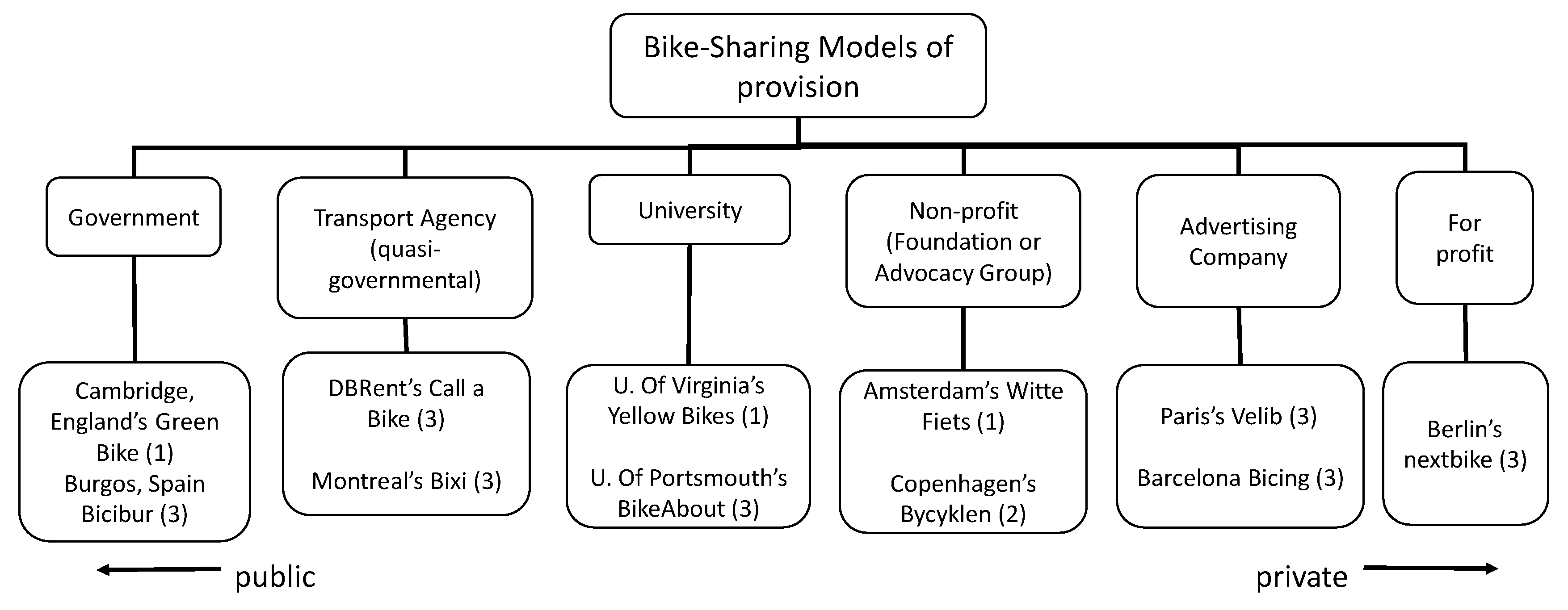
BSS is a dynamic system which highly depends on the operators. As illustrated in Figure 1, BSS providers have included governments, quasi-governmental transport agencies, universities, non-profits, advertising companies and for-profits [9]. While the for-profits operate by a private company with limited or no government involvement (e.g., NextBike), the government model is located in the opposite direction (e.g., Bicibur). The model expresses that operators would affect the operational factors. For example, private sectors of BSS are likely to have more services than the public sectors since it runs with the intention of making a profit. Failure examples exist and cause anxieties on the new establishment of similar programs regardless the operators. For example, the operation termination of bike-share Helsinki in 2010, which then returned in operation in 2016 [10] and Argonne National Laboratory are some of the cases of [11]. To overcome such worries, many bike-share operators have deployed a standard of efficiency-related performance measures such as daily usage and density. Daily usage refers to the number of trips per bike per day while density denotes as the station density and population density in the region as the coverage area. For example, the sustainability of such program in most other schemes internationally has been reported that the usage rates ranged between 3 and 6 trips per bike per day [12]. CitiBike cited that each bike is ridden 8.3 times a day with 6.7 daily trips per bike [13] and Copenhagen’s Bycyklen has only been used 0.8 times a day by tourists and failed to comply with the operational costs [14]. For the density, Institute for Transportation & Development Policy has set an essential planning and design guideline with station density are 10–16 stations per km2 and population density is 10–30 bikes for every 1000 residents [15]. Although the frequency-based and density-based measures are generally used to describe the productivity in the BSS, it sometimes fails to measure the sustainability of BSS.
Another model of BSS can be expressed based on the checkout time, namely bike library systems. Bike Library System is considered as a system that allows one person to use long-term checkout by keeping the bike for several months. This particular type of BSS might have a less desirable result with frequency-based measures since the measure would give a misleading information with a lower usage frequency, around less than three uses per day on average, in comparison to more than six uses per day on the typical BSS. In other words, time aspects as one of the attributes existing on the trip data have not been properly utilized. An alternative measure is necessary to understand how effective the bikes in the respective systems. The measured result would show the effectiveness and efficiency of bikes as well as to address BSS sustainability. Hence, rather than measuring the performance based on frequency, this study considers the bike assessment based on the time aspect.
This study aims to propose a measurement for assessing bike effectiveness, named as OBE. OBE, inspired by OEE, has also applied availability, performance and quality. Other work had proposed a similar approach for transportation, namely Overall Vehicle Effectiveness (OVE) and Overall Transportation Effectiveness (OTE). A bike has been considered as one of transportation modes which the nature of non-motorized transportation (or less polluting transport due to the existing of e-bike) requires specific methods for the measures. Hence, the contributions of this study lie in three salient aspects. First, unlike the existing transportation measures that include the direct environmental impact (e.g., emission), the proposed measure focuses on the utilization aspect, i.e., time, to prevent indirect environmental impact such as the high cost of BSS operation termination. Second, the public-use bike allows single capacity with the dynamic time schedule, unlike the public (scheduled) transportation. Finally, BSS follows complex dynamical system, unlike public transportation that follows a journey pattern. Three factors are considered to differentiate this study and the other transportation modes as the basis of the measurement; durability, attractiveness and practicality [15]. Durability is considered as a measure of real systems with values that express long duration based on time units [16]. In this study, the durability of a bike can be measured by the duration of the active bike. The attractiveness of a bike refers to the frequency of a bike that has been used. In term of practicality, it is difficult to measure since the criterion is about the physical of a bike. In particular, a bike probably has more sub-items for some other purposes. For example, a bike with a front basket can be used to carry bags, packages or groceries. Although there might be other factors that affect user’s choice on a bike, those three categories represent most cases of the effectiveness [15]. Since the practicality is followed by citizen’s culture and riders’ requirement that may diverse among BSS, the scope of this study focuses on durability and attractiveness aspects.
To summarize, this study has three main contributions as follows:
- -
- To propose the overall bike effectiveness (OBE) derived from OEE and OTE.
- -
- To measure the BSS sustainability using OBE and Theoretical-OBE (TOBE).
- -
- To experiment the proposed measure based on the real dataset.
The specific research question of this study is how to measure the performance of BSS based on the bike perspective? This analysis is undertaken in the context of establishing sustainable bike-sharing systems. The concept of sustainability mentioned in this study is to understand the well-establishment of the system as well as the contribution to the product, i.e., bike and life-cycle. The analysis result does not imply the economic perspective such as government- and private-funding as well as public-funding in the form of subsidies.
This paper is organized as follows. Section 2 addresses the existing approach in OEE and performance measures in BSS. Section 3 describes the proposed approach. Section 4 illustrates the implementations and analysis result. Section 5 shows the value proposition of the proposed approach. Finally, Section 6 concludes this study.
2. Literature Review
This section addresses literature reviews related to the sustainability issues of BSS, the challenges of achieving the objectives and approaches for measuring bike performance. In addition, this section includes reviews of OEE measurement on the transportation domain as well as the integration of transportation indicators into the OEE.
2.1. Issues of Sustainability in Bike Sharing System
BSS is emerging as a cost-effective and sustainable approach to expanding transit options. The regions that implement BSS are aware of the benefit in the economics, environment and public health when the program is structured with incentives on short-trips. Williamson addressed three aspects of sustainability of BSS; economic, social and environmental [17] while other addressed the issues on noise and/or pollution as well as the consumption of less non-renewable resources than motorized transportation mode [18]. Due to the rising of BSS in many big cities around the world, transport policies to support the sustainability of BSS would be necessary to maintain the operation avoiding the risk of termination [19,20]. In addition, the sustainability of BSS has merely discussed the balance between physical design of the system and the provision of services being offered as a Product Service System (PSS) [6,20]. Performance measure would be carried out to help operators maintain the bikes life-cycle which was paid less attention initially.
A number of previous works had been dedicated to promote bike availability and provide better cycling facilities to improve the BSS. In the operational aspects, most studies focused on the location-allocation problems such as determining location of stations [21], predicting bike availability [22], while other works evaluate the BSS in terms of rack utilization [23], balance of bike availability [24,25], mobility patterns [26], speed and path characterization [27] and optimization of bike planning and utilization [28]. Most of them worked on the sustainability approach, such as resources and economic factors without considering the performance measurements. While the policies, systems and resources are significant to highlight the degree of sustainability in the society, there is still a challenge to identify the speculation of operation termination. In addition, the bike life cycle has been less-considered issues since the initiation of the third era of BSS using technology to control and monitor the mobility of bikes. Moreover, BSSs serve as PSSs which provide cohesive delivery of products and services.
The provision of performance metric, specifically for bikes, is necessary for two reasons. Firstly, it shows the effectiveness of bikes throughout the time period of the service. In another word, the durability of bikes as one of the critical success factors of BSS would be measured. Secondly, the quality of bikes throughout the time period would also be perceived. In term of attractiveness, some of the bikes which remain either idle or low in utility would be detected. This background would be the basis to develop metrics towards the sustainability of BSS.
2.2. Overall Equipment Effectiveness on Transportation
The initial OEE indicators have been developed to measure the implementation of Total Productive Maintenance (TPM) [29]. The implementation has been included as one of six techniques used by the lean production [30]. In short, OEE is determined according to the equipment (i.e., machine) used in a production process to identify its availability, quality and performance contributions. The possible relationship among indicators has also been considered [31]. As the definition where efficiency is doing the right things and effectiveness is about doing things right; some works focus on measuring the efficiency rather than effectiveness [32]. Commonly, OEE is used for production performance monitoring as part of performance measurement systems. In particular, the indicator can be used to identify the worst performing machine for TPM [29,30]. The used of OEE has been applied in some fields such as to improve the productivity of the respective equipment [33], utilization indicators in the aerospace industry [34] and to analyze equipment’s reliability [35]. The measurement using OEE can also be applied into factory (Overall Factory Efficiency (OFE) [36], layout (overall space effectiveness (OSE) [37], labor (Overall Labor Effectiveness (OLE)) [38], equipment productivity (overall tool Group Efficiency (OGE)) [39], equipment and system productivity (overall throughput effectiveness [40] and product-based level such as wafer (overall wafer effectiveness (OWE)) [41].
The term value-added is introduced when using the OEE in non-manufacturing environments. Value-added effectiveness (OVAE) could be used as an alternative to measure the effectiveness of the services [42]. Some studies have been concentrated on measuring transportation performance. Overall Vehicle Effectiveness (OVE), which is based on the OEE, was proposed to measure rigidly the effectiveness of transportation to identify improvement gaps in the relation to three indicators, i.e., availability, performance and quality. A framework of Overall Transportation Effectiveness (OTE) was proposed to solve the problem in a specific domain such as transportation [43]. The framework can be used from a vehicle (i.e., truck) perspective and drill down to levels and categories of transportation effectiveness to steer on the strategic, tactical and operational level and visual performance.
Although previous studies have attempted to establish a measure for vehicle and transportation aspects, the concepts are different from OBE. Firstly, frameworks such as OVE and OTE are conceptualized to measure the performance of vehicles which purposely proposed for vehicle or transportation modes related to industries, e.g., CO2 calculation at the trip level. Meanwhile, the BSS is a semi-public “green” transportation that varies from the social and culture of the city that they belong. Second, the measures of loss identification and effective trip detection are two different things. The OTE has been intended for logistics (Logistics Service Provisioning) which has challenges in profit and loss in terms of economy-environment aspects, while BSS is mainly aimed to public transport with socio-economic-environment aspects. For example, government model BSS would consider assessing the bike availability and effectiveness, more than profit and loss of the systems.
A study on the performance of Overall Service Effectiveness (OSE) in urban public transport had been carried out previously [44]. The study proposed a method to measure the bus services as the category of scheduled transportation where in scheduled transportation, service time is prearranged. In addition, the number of occupied seats will be taken into account as one of the performance measures. Meanwhile, the bike performs as a single capacity fleet and the service time highly depends on the riders. The difference of nature between scheduled transportation and bike is the distinguished points of this proposed method. Using the OEE concept, this study focuses on bikes as an entity for measuring the effectiveness.
The work of [4] showed that one of the major barriers of BSS was when users had no interest in biking. Bike operators have been aware of these reasons, such as a lack of convenience, competitive advantageous with other modes, safety concerns and anything that hinders the freedom of choice. Improving the aforementioned factors would encourage citizen to use the bikes. Many bike-share organizations rely on the measure of the average of bike trip per day to measure the effectiveness of BSS. In addition, the increment of BSS performance is indicated by using the number of trips. Although the measure could represent the effectiveness of the BSS, it only considers the frequency rather than the time aspects of the bike. For example, the concept of the bike library system could not be detected with the measure. OBE—on the other hand, it applies the time duration as one of the attributes used to consider the effectiveness of the BSS. Consistency and improvement are two key measures to check the BSS performance. While consistency requires a stable indicator from the time-to-time basis, improvement should show a trend in time-to-time basis. The proposed OBE metric could be one of the approaches to see the consistency and improvement of the respective BSS. Furthermore, the result can be shown as an evaluation measure to present the effectiveness of bike usage and effective trip. This form of evaluation could identify and compare the respective BSS with other similar BSS as the critical improvement directions. Therefore, this study attempts to compare between the OBE and the common measure, which is the average trip.
3. Proposed Metric
This section addresses the new metric—named OBE—which is based on the OEE (Equation (1)).
OEE = Availability × Performance × Quality
The OBE is the result of indicators used to include the calculation of availability, performance and quality in the respective of bike trips. The aim of this new metric is to identify the losses on BSS and establish a complete understanding of the BSS in terms of availability, performance and quality. The identification and measurement of these efficiencies allow the operator to implement the necessary corrective actions to improve the service.
3.1. Formal Definition and Running Example
Most of the BSS will record data of the bike ID, start time of the trip, end time of the trip, duration of the trip (in second), origin station, destination station and some other external attributes such as riders profile, station ID, zip code, etc.. This study uses only the relevant attributes to enhance the effectiveness measure. Table 1 shows the fragment of bike trip data used in this study. Note that the time granularity used by most BSS is at the level of minutes while the duration is recorded in seconds. Formal definitions are required to express the time aspects on BSS.
Let E be a set of trip of bikes. A trip log (L) is a collection of trips represented as a tuple of the form bike ID, start trip (ST), end trip (ET), duration (D), origin station (SS), destination station (ES) and rider’s type (U). Note that the riders’ type consists of customer and subscriber. The former refers to the general rider while the latter denotes riders who subscribe as the BSS members. A sequence of trip is denoted as σ = <e1, e2, ..., en> E* where each ei denotes the i-th trip of a bike and n ∈ denotes as the total trip within a period of time.
Suppose that S is a set of stations, thus SS ⋃ ES is a subset of S. The notation e.id, e.st, e.et, e.d, e.ss, e.es, e.u are used to represent bike ID, start trip time, end trip time, trip duration, origin station, destination station and rider’s type, respectively. For example, e = (“1”, “2015-02-24 11:24:00”, “2015-02-24 11:31:00”, 425, A, B, “Subscriber”), then e.id = “1”, e.st = “2015-02-24 11:24:00”, e.et = “2015-02-24 11:31:00”, e.d = 425, e.ss = “A”, e.es = “B”, and e.u = “Subscriber”.
To indicate the bike, the notation k = 1, …, K is used to represent the k-th bike. Hence, a sequence for the trip of bike k is denoted as σk = <ek1, ek2, ..., ekn> ∈ E* where eki ∈ E is a single trip for 1 < i < Ik and Ik is the total trip of the k-th bike. Referring to Table 1, bike ID #1 (k = 1) has five trips (called the actual trip frequency) and it can be denoted as I1 = 5.
As illustrated in a frequency-based measure by many BSS, it takes into account the actual trip frequency. The total trip frequency of all bikes is commonly used as a measure to indicate the popularity of the BSS. Rather using the total trip frequency, this study uses ratio to represent the BSS performance. Rate (Rk) is the ratio of actual trip frequency (Ik) with the best trip frequency, referred to the maximum of actual trip frequency among the active bikes K (Equation (2)).
3.2. Definition of Overall Bike Effectiveness (OBE)
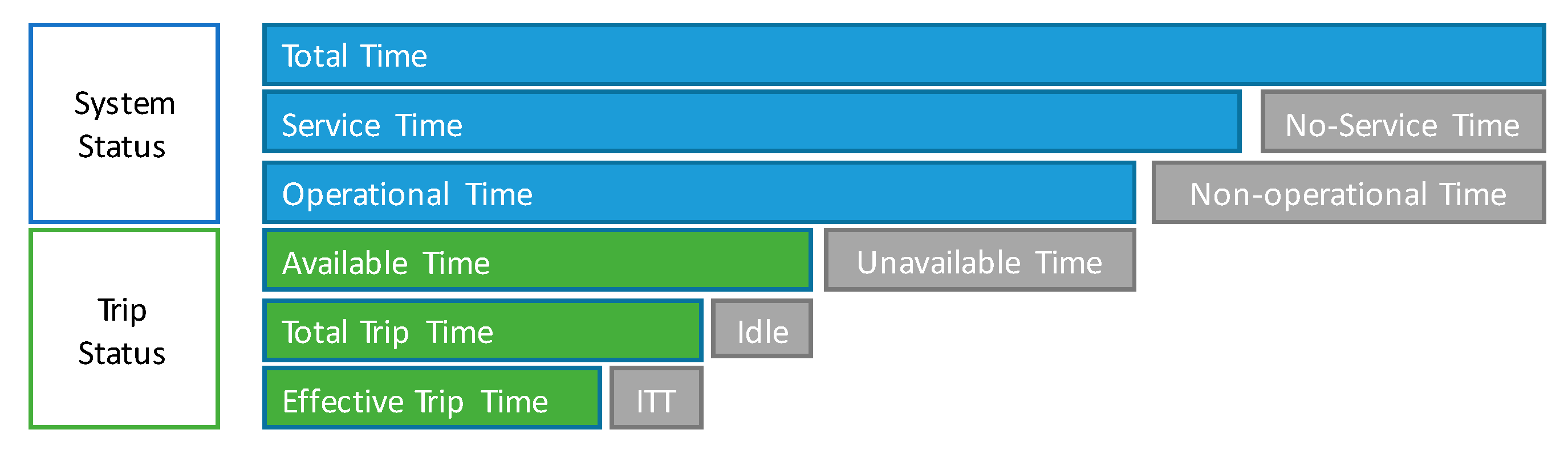
OBE is a term with some metrics to evaluate the effectiveness of BSS. There are six basic time statuses, including total time, service time, operational time, available time, total trip time and effective trip time. Each of the statuses corresponds to an operational state of a particular BSS and a bike. Thus, OBE indices can be defined with system status and trip status. In detail, the OBE framework with regard to time is illustrated in Figure 2.
System status refers to operational information from the BSS. Meanwhile, trip status is derived from the trip data provided by a particular BSS. Generally, there are three system statuses in BSS; total time, service time and operational time. These statuses focus on the BSS operational aspects as a resolution for improving bike effectiveness. The other three statuses, i.e., available time, total trip time and effective trip time refer to the trip or operational views. These statuses would be used as the basis for assessing the performance measure using OBE.
Total time refers to a particular time period for performance measures. A selected time period, i.e., a week, a month, a year, can be a reference for the basis of the analysis. The total time can be divided into two, i.e., no-service time and service time, to identify and analyze hidden performance loss. Service time refers to the time when the BSS operates. The loss in this time is labeled as no-service time which refers to the time limitation of the system due to public policy in each respective city. For example, BSS in Rio de Janeiro opens the service from 6.00 a.m. to 10.00 p.m. Therefore, the no service time equals 8 h/day. In the case of weekly basis analysis, the service time of the framework would be ((24 h − 8 h) × 7 days) = 112 h. In a different aspect, service time can also be considered as a virtual period when a user requires reserving a bike to ride on. For example, Grid bikes will allow the user to reserve a bike at a particular time [45]. In this study, the service time refers to the real-world time.
Operational time (O) can be defined as the time on which a bike can be used. Some scheduled maintenance can be one of the reasons on service time reduction which refers to the losses labeled as non-operational time. Although maintenance issues take important roles on the performance measures, it is difficult to specify the exact execution time. If such information is not available, the service time could be directly regarded as operational time.
Available Time denotes the time of a bike liveliness (i.e., in an available state) during the operational time. In other words, the available state refers to the time when a bike keeps performing on the system and is ready to be used. In contrast, the unavailable state is the time when the bike is unavailable from a particular time point in the respective of time analysis unit. These states, available and unavailable, are purposely for measuring the bike availability. Hence, the available time of k-th bike (ATk) can be derived by subtracting the end time of the last event with the start time of the first event of a particular bike. Bike Availability of k-th bike (Ak) is the proportion of bike available time in regards to the operational time. To measure the bike availability of the system, average bike availability is used. Average Bike Availability () can be derived by summing all k-th bike available time and dividing it with the available bikes (K) in the period. Note that the available bikes in the period could be different with the available bikes in other period due to the non-operational time such as maintenance. Equations (3)–(5) show the formula to measure bike available time, bike availability and average bike availability, respectively.
Average Bike Availability () can be regarded as a measure to ensure the availability of bikes in the system during the operational time. The can be used to understand any situations which cause low availability. For example, severe damages of bikes without any further action from the operator could cause an unavailable state in the stations.
Table 1 shows there are seven available bikes during three days of operational time. The available time of bike #1 (AT1) was derived by subtracting the end trip of the last event (“2015-02-26 22:51:00”) with the start trip of the first event (“2015-02-24 11:24:00”). Hence, the AT1 is 3567 min. The A1 (the availability of bike #1) would be a division of AT1 with the operational time (3567/4320 = 0.8256). Finally, the bike availability of the respective BSS () is measured by dividing the summation of all bike availability with the number of available bikes. Thus, the bike availability is 49.49% (refer to Table 2).
Trip time is the duration of a bike used by a rider. In some BSSs, the trip time has been stored in the time unit of ‘second’ as a trip duration although the trip data includes the starting and the ending time of one bike along with riders and stations data. Hence, the total trip time of the k-th bike (TTTk) is the summation of the trip time of k-th bike in the period. To measure the bike performance, it is necessary to know the maximum (best) trip time (TTTbest) in the system in a particular period.
There are two ways to determine the best total trip time () based on the period p. First, the value can be determined by selecting p as the best period in the previous year. For example, if the current period of analysis is March 2014, then the period p refers to the month in the previous year which returns the best value. Second, the p could refer to the same period of the previous year, or year-over-year basis. For example, if the current period is March 2014, then the period p refers to March 2013. The first approach has less accuracy than the second approach due to seasonal aspects, i.e., weather differences, particular events, etc., with the respective period. In addition, the selection of p can be different among BSS in accordance to the factors that the operators want to analyze. Hence, the performance of the k-th bike (Pk) is the fraction of total trip time (TTTk) and the best total trip time in the system (TTTbest). Average Bike Performance () can be derived by summing all k-th bike performance and dividing it with the available bikes (K) in the period. The Equations (6)–(9) show the total trip time, the best total trip time, bike performance and average bike performance, respectively.
In many cases, the BSS records the duration of a trip. Since some of the BSS stored a coarse-grained time data (i.e., the smallest time unit is stated as ‘minute’), the duration would be more representative to express the fine-grained time data. For example, the first trip of bike #1 has a duration of 425 s meanwhile the difference between the start trip and the end trip result 420 s. By summing all the duration of the bike #1, the total trip (TTT1) is 1,996 s during 3 days operational time. The maximum of trip time among all bikes are the bike #6 which reach 14,580 s, assuming that there is no previous year data. Hence, the bike performance (P6) of bike #6 is 100% and other bikes’ performance follows each of the trip time. Finally, the average of bike performance is evaluated by dividing the summation of all bike performance with the number of available bikes in the period.
Effective Trip Time is the trip time when a bike is properly used during the trip. To measure the effective trip time, it is necessary to understand the ineffective trip time. There are two types of the ineffective trip; ineffective loop trip time and low utility trip. The ineffective loop time of the k-th bike (ILTk) denotes a trip which (1) the destination is the same as the origin (loop trip) and (2) short trip time. For example, a rider may discharge a bike from a station and return it to the original station due to some problems, e.g., flat tires, which rise the rider’s unsatisfactory. The low utility trip of the k-th bike (LUTk) refers to a trip which the TTTk in the analysis period including the frequency of bike usage is less than the standard set by the operator. There are two types of low utility trip; low utility total trip time and low utility trip frequency. For example, the operator sets a bike should be used at least 5 times and more than 60 min of total trip time in a day. Otherwise, the bike is considered as having an ineffective trip time due to the low utility trip. Hence, the effective trip time of k-th bike (ETTk) can be derived by subtracting the total trip time (TTTk) with the ineffective trip time (ITTk). Note that the ineffective trip time is the summation of the ineffective loop trip and low utility trip. The notion of quality of the k-th bike (Qk) means the fraction of effective trip time from the total trip time of the bike. Average Bike Quality () can be derived by summing all k-th bike quality and dividing it with the available bikes (K) in the period. The Equations (10)–(15) describe the ineffective loop trip, low utility trip, ineffective trip time, effective trip time, bike quality and average bike quality, respectively.
The notation , and refer to the threshold for ineffective loop trip, low utility total trip time and low utility trip frequency, respectively. Note that those thresholds would be determined by the BSS operators and varied according the implemented BSS. BSS which applies free-of-charge pricing structure on the earliest hour of rental would have different threshold with other BSS. For example, Barcelona BSS and most United States (US)-based BSS consider the first 30 min of rental as free-of-charge [15]. However, YouBike (Taipei) charges the riders from the first time the bike discharges from the station [46]. Hence, the ineffective loop trip time would be varied according to the policy of the local BSS. For the low utility trip, the thresholds would be based on the target of the BSS operators. For early stage of BSS, operators could not set a high standard. When the BSS becomes stable, operators can increase the threshold to improve the BSS. As a result, the OBE of the k-th bike is referred to the product of bike availability, bike performance and bike quality expressed as Equation (16). To obtain the overall performance of the BSS, the average of OBE is derived as denoted in Equation (17).
The fragment data in Table 1 would be used to illustrate the calculation of OBE. A visualization for explaining each of the terminology mentioned in Figure 2 can be seen in Figure 3. The calculation begins by determining the operational time and subsequently measures the performance within three statuses; available time, trip time and effective trip time. The total time would be determined by the analyst. Table 1 illustrates a BSS with a total time of 3 days (4320 min or 259,200 s). Assuming that the BSS operates in 24 h, the service time is considered the same as the total time of 3 days. Since no particular information about maintenance and other issues on operating hours during the period of the fragment trip data, the operational time is considered being equal to the service time.
Measuring bike quality begins by identifying the low utility trip and ineffective loop trip. In many cases, this identification is a challenging assessment since it is hidden in the bike trip. Note that this calculation example is based on a small dataset from Table 1. The threshold could be set either manually by operators or statistically measured from the data. For example, the low utility trip frequency is lower than or equal to the average of the frequency of all bikes (e.g., 3.4) and the low utility total trip time of each bike is lower than a value, e.g., a standard set by the operator. Assuming that a daily trip time should be greater than 300 s. Since the operational time of the dataset is 3 days, the threshold will count 900 s. Hence, the bike ID #4, #5 and #7 are in the category of since the total trip time of the three bikes is less than 900 s. The ineffective loop trip is measured by pointing a trip that has the same origin and destination and is less than 119 s. Note that the basis of this measure varies according to the policy of BSS. Based on Table 1, bike ID #1 has 1 occurrence of ineffective loop trip with a duration of 118 s. The effective trip time is derived by subtracting the total trip time with low utility trip and ineffective loop trip. The quality of bike #1 is assessed as (1996 − 118)/1996 = 0.9408. Using the same ways as other bikes, the is 56.29 which is obtained as the average of Qk from all bikes.
The overall bike effectiveness of each bike is the multiplication of the three factors. For example, the OBE of bike #1 is 82.56% × 13.68% × 94.08% = 10.62%. Hence, the OBE, as the overall bike effectiveness of the BSS, is the average of the OBE of all bikes, 8.94%. Note that it is rare to get 0% of the k-th bike OBE in the real world data. However, the existence of 0% of OBE would be very important analysis for the operator to improve the BSS. The detail time derivation for effectiveness calculations is illustrated in Table 2.
3.3. Directions for Enhancement—Theoretical-Based OBE
The proposed OBE frameworks and indices basically align with a stable BSS. As aforementioned, the newly established BSS is limited on determining some parameters, i.e., the best total trip time (TTTbest) within a period of time. In addition, the bike available time on the new BSS would be less than the stable BSS. As a result, the OBE result would be very low and probably mislead toward termination action. Hence, alternative measures to represent the performance of early generated BSS is necessary. This section addresses the directions for enhancement of actual-based OBE toward theoretical-based OBE (TOBE).
Some newly established BSSs would have many issues on the availability since it requires weeks or even months for introducing the benefit to the society. In the early stage of the BSS, there would be fewer riders which will indirectly reduce the available time and increase operational cost. As a consequence, theoretical-based measurement is likely useful to assess the effectiveness of BSS. However, determining the bike available time would be an issue of measuring the bike availability. Rather than using the actual-based measure, the early stage of BSS could apply the theoretical-based measure. In this case, the theoretical bike availability (TA) is obtained by calculating the proportion of a number of available bikes (K) in the period with the number of installed bike provided by the operators (κ).
Note that the number of installed bikes refers to the number of fleets provided by the operators in the respective BSS. The number of available bikes could be assessed by extracting the bike used by riders within a period of time. If the number of available bikes the same as the number of installed bikes, then the TA is 100%. The loss would be caused by maintenance or replacement issues in a particular period.
The early stage of BSS is also likely to have performance stability issues in comparison to the stable BSS. Measuring the best total trip time is less considered due to instability. Instead, theoretical bike performance (TP) can be assessed based on the target trip frequency (TTF). The TP would be the fraction of average actual trip frequency to the target trip frequency.
Actual trip frequency is the number of actual trips of a bike in a particular period (e.g., monthly basis) while the target trip frequency is the target frequency of bike trips in a period determined by the operator. If the actual trip frequency is the same as the target trip frequency determined by the operator; then the theoretical bike performance (TP) is 100%. The loss in this performance could be highlighted as three fundamental interrelated exogenous factors such as bike-ability and safety, the institutional ownership types and the physical design factors [47].
In regard to the quality aspect, there would be no issue on low utility trip and ineffective loop trip if all bikes in the early stage of BSS are in good conditions. Although there might be other factors in quality issues (e.g., infrastructure), the theoretical bike quality (TQ) could be considered the same as . By applying the same measure as , the TQ tends to have a high rate, i.e., 100%.
For assessing the TOBE, the fragment data (Table 1) would be used. Suppose the operator installs ten bikes and only seven bikes are available in the three days period. Hence, the TA is (7/10) × 100% = 70%. The TP is measured according to the target trip frequency determined by the operators. Suppose the operator targets 5 daily trips per bike. Referring to Table 2, the TP is (3.43/5) × 100% = 68%. Note that 3.43 is the average of the actual trip frequency of the available bikes. Finally, the TQ remains the same as and the value is 56.29%. The TOBE originates from the multiplication of the three perspectives which give the result of 26.79%.
4. Case Study
This section is aimed to show the effectiveness of the proposed approach in a real data of BSS. First, the dataset in this study is introduced. Subsequently, the periodical analysis in a respective year is also analyzed.
4.1. Data Introduction
A dataset of San Francisco (SF) Bay Area Bike Share is used for the case study. The reason behind choosing the SF dataset is the popularity of the BSS [48] as well as the provision of the dataset [49]. According to the latest information, there were about 700 bikes in the beginning of the operation and are currently about more than 1000 bikes in the system with the future plan as about 7000 fleets in 2017 [50]. The operation time of the SF BSS is 24 h, seven days a week. A rider may have unlimited trips of up to 30 min which is measured from the time the bike is discharged from a dock to the time the bike is returned without any cost. Since the BSS offers services for individual short trips, longer trips incur additional cost. A replacement fee would be charged to the rider when the bike is lost during the rent.
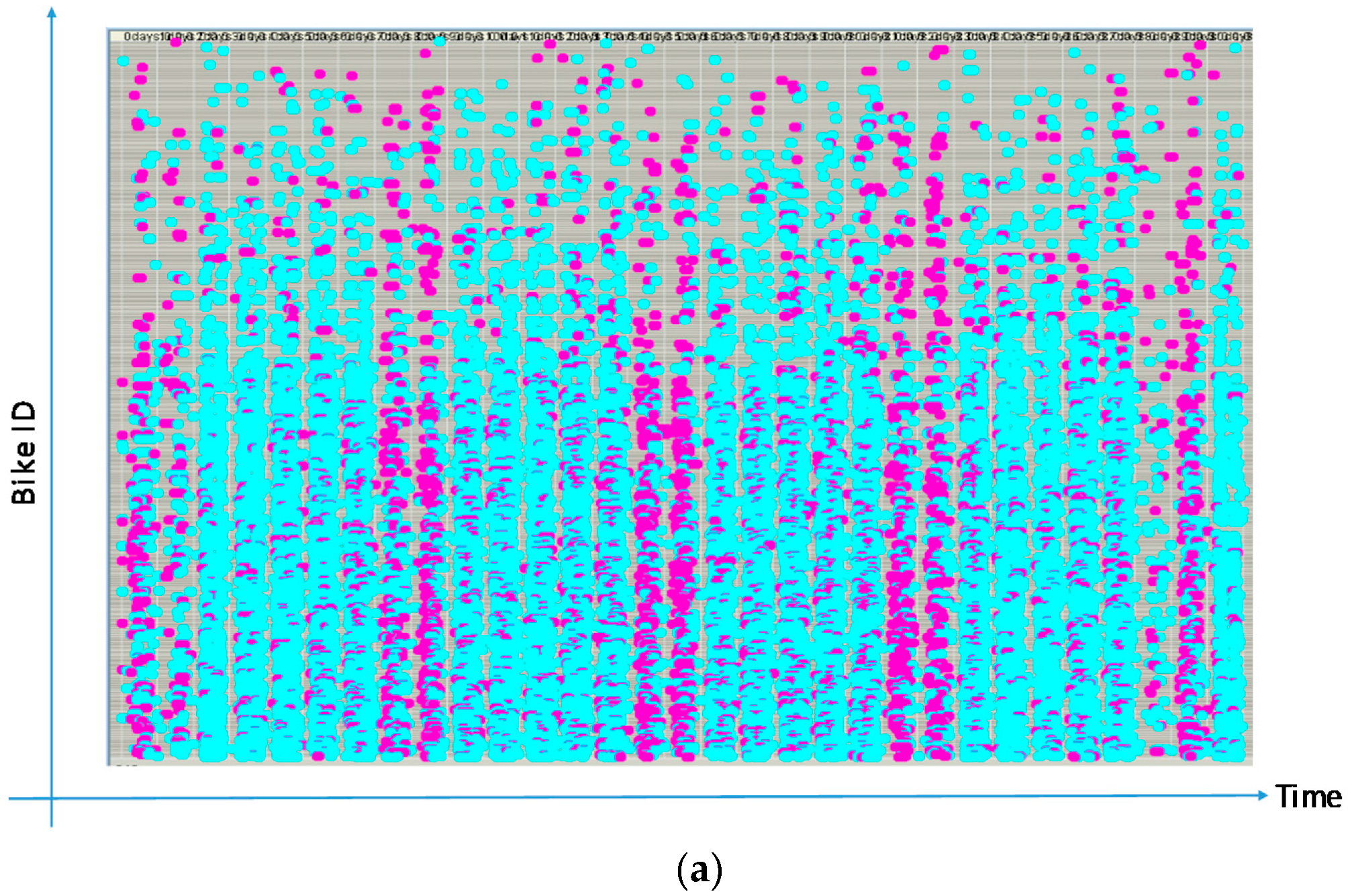
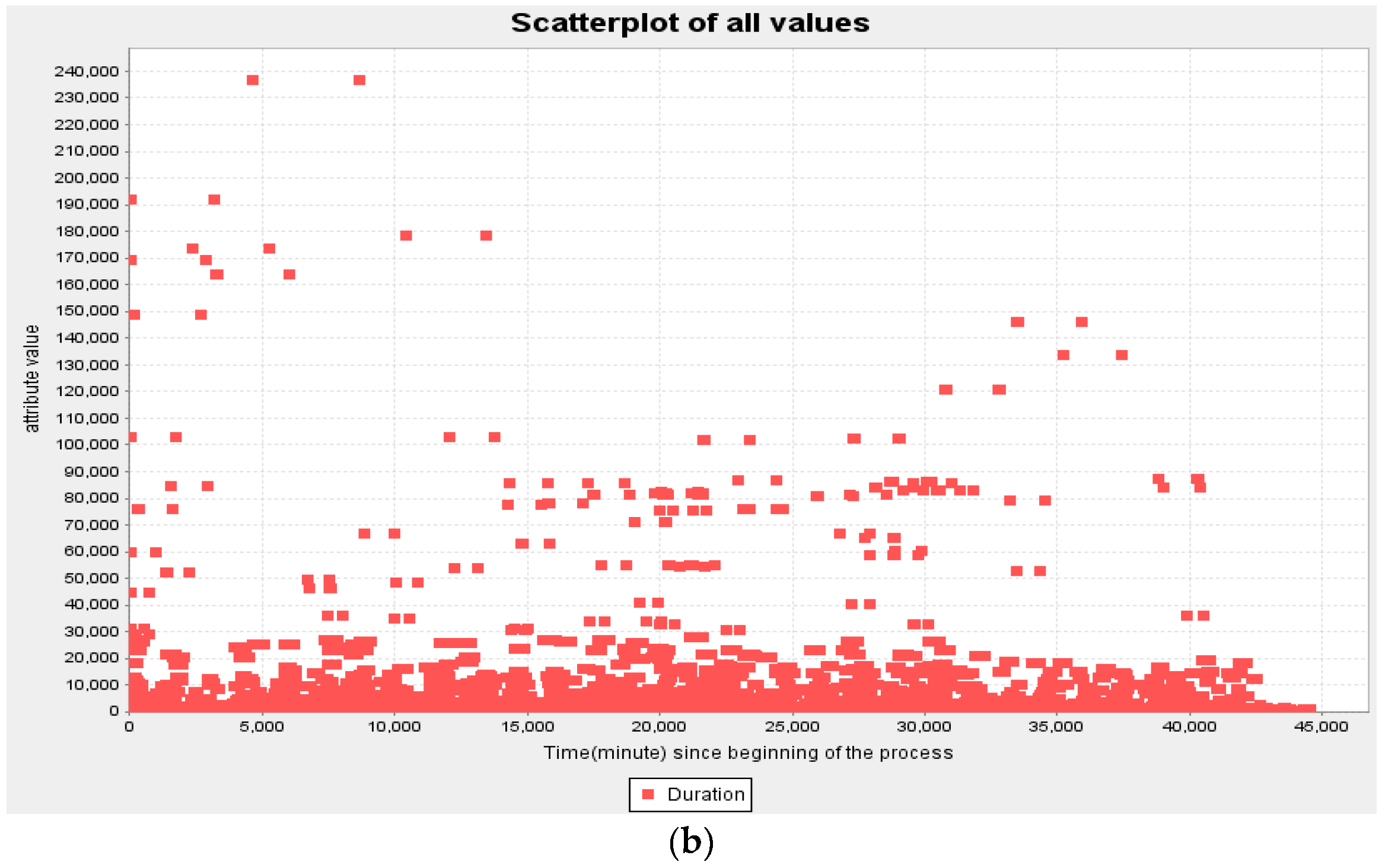
Bay Area Bike Share (now turn as Ford GoBike) had announced their first open-data challenge in 2014 [51]. Although there are many insights on the trip analysis such as time-based exploration of bicycle trip data, it remains a challenge to the bike perspective analysis toward sustainability of the BSS. Figure 4 shows a preliminary insight on the analysis of bike effectiveness, in terms of durability and attractiveness. Dotted plot (Figure 4a) aims to show the performed events within relative time perspective. Using a monthly data of SF BSS (March 2014), the dotted plot shows the effectiveness of the bikes which blue and pink represent the event patterns of subscriber and customer, respectively. The dotted plot also shows the distance between events which represent the idle state. Since there are a lot of bikes involved in a BSS, it is necessary to develop a method to measure ineffective trip of bikes toward OBE. Figure 4b displays the scatter plot that indicates the duration of the trip for all bikes from the beginning period of the analysis. The scatter plot refers to the time duration (in seconds) of bike riders’ trip. Some bikes had been used more than 150,000 s (1.7 days) and many of them were used in short duration. This means that the BSS do serves riders for short trips and the assumption that bike had been used for the short-trip should be extended towards bike library system.
4.2. Analysis Result
The result is categorized into two categories; the frequency-based and time-based measure. Frequency-based measurement applies the Rate measure using the ratio of the actual trip frequency. Meanwhile, the time-based measure applies OBE which considers the trip time of bikes. As the common measure of BSS, the Rate measure would be compared with OBE using some quantitative ways such as plotting and statistical analysis.
Before conducting the analysis, the dataset is filtered according to the analysis time period, i.e., monthly. The method to filter the dataset is to select the bike that has start time after the beginning of the month and has the end time before the end of the respective month. The filtered process takes place to ensure that the dataset includes at least a trip.
Figure 5 displays the plot to show the relationship between bike performance (called as Performance in the chart) and Rate. High-performance utilization can be seen as high usage and equal to the bike which has maximum trip time in a particular period. The comparison between the two identifiers classifies the correlation between time-based and frequency-based performance. Moreover, it reflects some categorizations of BSS; durability and attractiveness. For example, short time performance and high frequency of a bike represent the effectiveness of a BSS to be a short trip (last mile) transport system. On the other hand, long-time performance and low frequency illustrate the bike library systems. The variation of each bike time performance would unclearly be seen unless the relationship of the three measures (availability, performance and quality) is analyzed.
Considering the SF data in August 2014, the correlation plot among the factors of OBE is performed (see Figure 6). This plot shows the details of the BSS performance in the respective measures. Two issues could be further discussed from this plot; outlier and patterns. The quality plot displays high values with two outliers. The top right element shows the best quality bike. Meanwhile, the bottom left element seems to have issues, e.g., bike damage. The diagram shows that the dots on the bottom-left has low availability as well as low performance. Using this correlation plot, a stakeholder can easily analyze the overall performance of BSS in a particular time period.
This would be advantageous to look at the density plot to investigate the monthly OBE patterns or the relationship between variables. Density plot could visualize the distribution of data over a continuous interval or time period. To clearly see the relationship of all variables, the density plot performs multiple groups of data, i.e., OBE, Availability, Performance and Quality. Figure 7 illustrates the density plot of all groups’ data of San Francisco BSS in 2014. Each graph displays the OBE in a period of one month. Note that the graph title “SF 1401” refers to the San Francisco dataset of January 2014 (14 is the year 2014 and 01 is the month). This graph title (as well as for the dataset name) is used throughout the analysis in this paper. From the graph, June, July and August showing the high demands of the BSS by observing the high-scale values of the OBE.
Having pointed out the values of metrics, the value of 1 represents the best performance of the measures. In regard to the availability, all months show high numbers of bike availability except in November, which is slightly lower than others. In respect of quality, all bikes show high quality since the values are approaching 1. However, some respective months such as March, May and June display a slight decrease in the quality. Bike performance is the measure that exhibits the variation among months. The right skew on the diagram with bi-modal distribution presented by the performance affects the distribution of OBE. Hence, OBE varies according to the distribution of three measures, availability, performance and quality in each month.
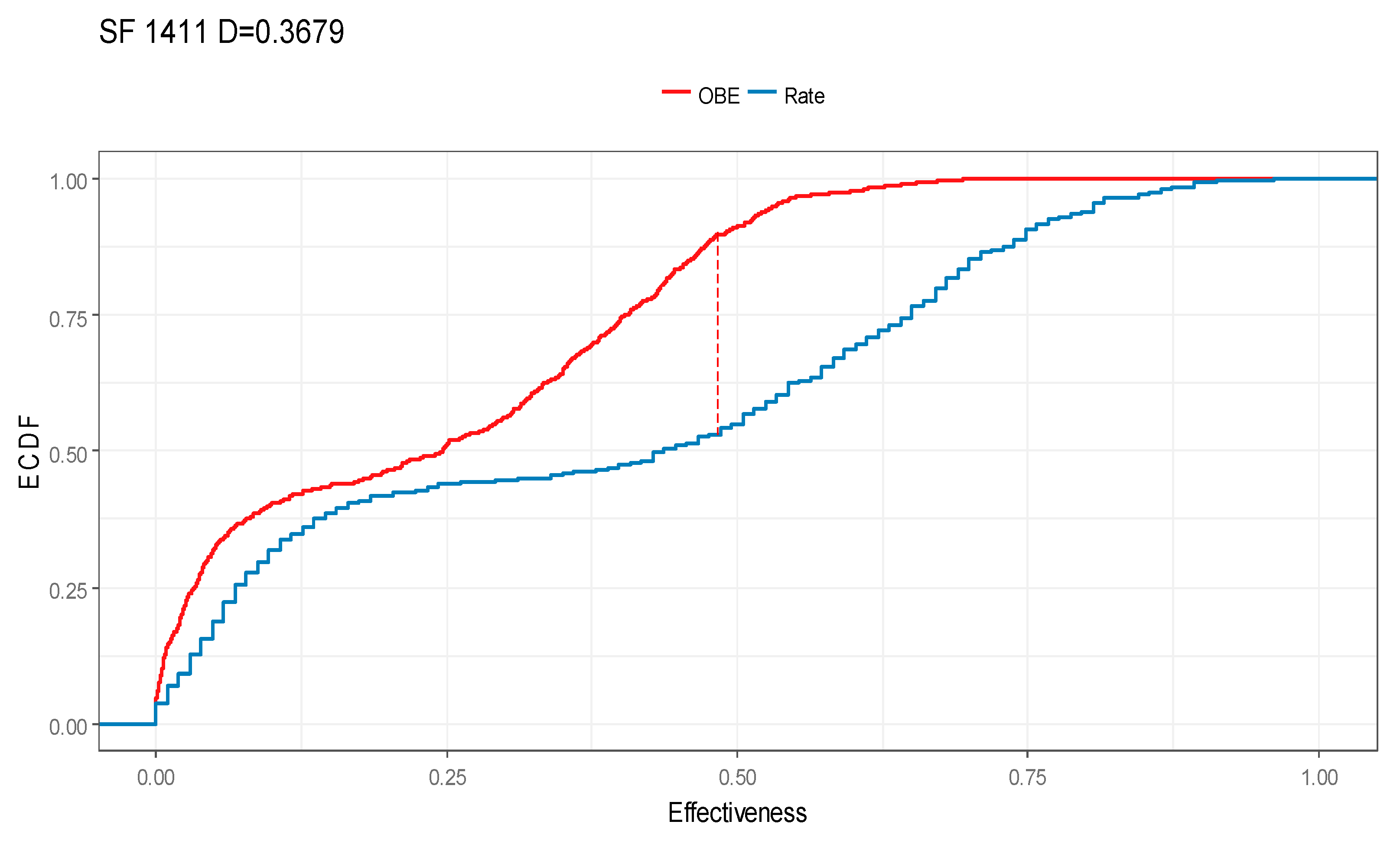
In order to show the effectiveness of OBE in comparison to the existing measure, which is Rate, it is necessary to analyze the equality of both measures. First, the density plot of OBE and Rate took place to see the difference between the two measures (see Figure 8). It shows that the Rate has bi-modal distribution with left skewness which means that the values are approaching the value 1 while the OBE is a bi-modal distribution with right skewness on which most the values are less than 0.75. The consideration of the time aspect could show the difference between the two. To clearly see the difference between two measures, a statistical approach is applied. One of the approaches in statistics to deal with comparing two samples of continuous data is Kolmogorov Smirnov Test (K-S Test). K-S Test is used to analyze whether the sample comes from a population with a specific distribution [52]. Based on the empirical distribution function (ECDF), it determines the maximum distance between two curves. Given N data points, Y1, Y2, …, YN, the ECDF is defined as
where ni is the number of points less than Yi. Using the two-sample K-S test, it compares two empirical distribution functions. That is,
In this study, two samples, OBE and Rate, are compared based on the SF 2014 dataset. The test statistic, δ, should be compared with the critical value. The hypothesis regarding the distributional forms is rejected if δ is greater than the critical value obtained from a table. Using 5% significance level, the table-based critical value is 0.175. Table 3 shows the test statistics value of each dataset. All δ values show greater values than the critical value. In other word, the OBE measure is significantly different with the Rate. Figure 9 shows the visualization of K-S Test of SF November 2014 dataset. The graph exhibits the rejection of the hypothesis and implies that there is a significant difference between the OBE and Rate measures. Hence, the time-based measure could show a different perspective of measures to show the performance of BSS.
5. Value Proposition
The proposed OBE can be used as performance indicators to measure bike effectiveness as well as to drive effective improvements from various aspects for bike operators, government and riders such as tourist, citizen, workers, etc. Furthermore, the OBE can be used for benchmarking, life cycle analysis, system evaluation and making strategy for sustainability.
5.1. OBE for Benchmarking
Many organizations use “best practice benchmarking” or “process benchmarking” to evaluate various aspects of their processes in regard to best practice. Success stories of particular BSS implementations encourage other regions to do “best practice benchmarking” to develop similar systems. For example, China has many big cities which have installed thousands and more of bikes. The success of BSS in Beijing, Wuhan and Hangzhou as some of the large BSS would be the model for developing the same systems. However, BSS in other areas such as Melbourne and Brisbane had issues in increasing the bike riders due to the convenient of motorized transport and docking stations which not being sufficiently close to home, workplace and other frequent destinations [8].
While the scheme scale might be different, some of BSS may have a similar business model. For example, the success of BSS running by private operators (e.g., iHeartMedia, Inc. as previously known as CC Media Holdings, Inc.) in Oslo had been an early iteration of which later installed in Barcelona. In other cases, the same operator runs similar size BSS in two areas of French (i.e., Caen and Dijon with 350 bikes). Accordingly, a particular measure for benchmarking among existing BSS is required.
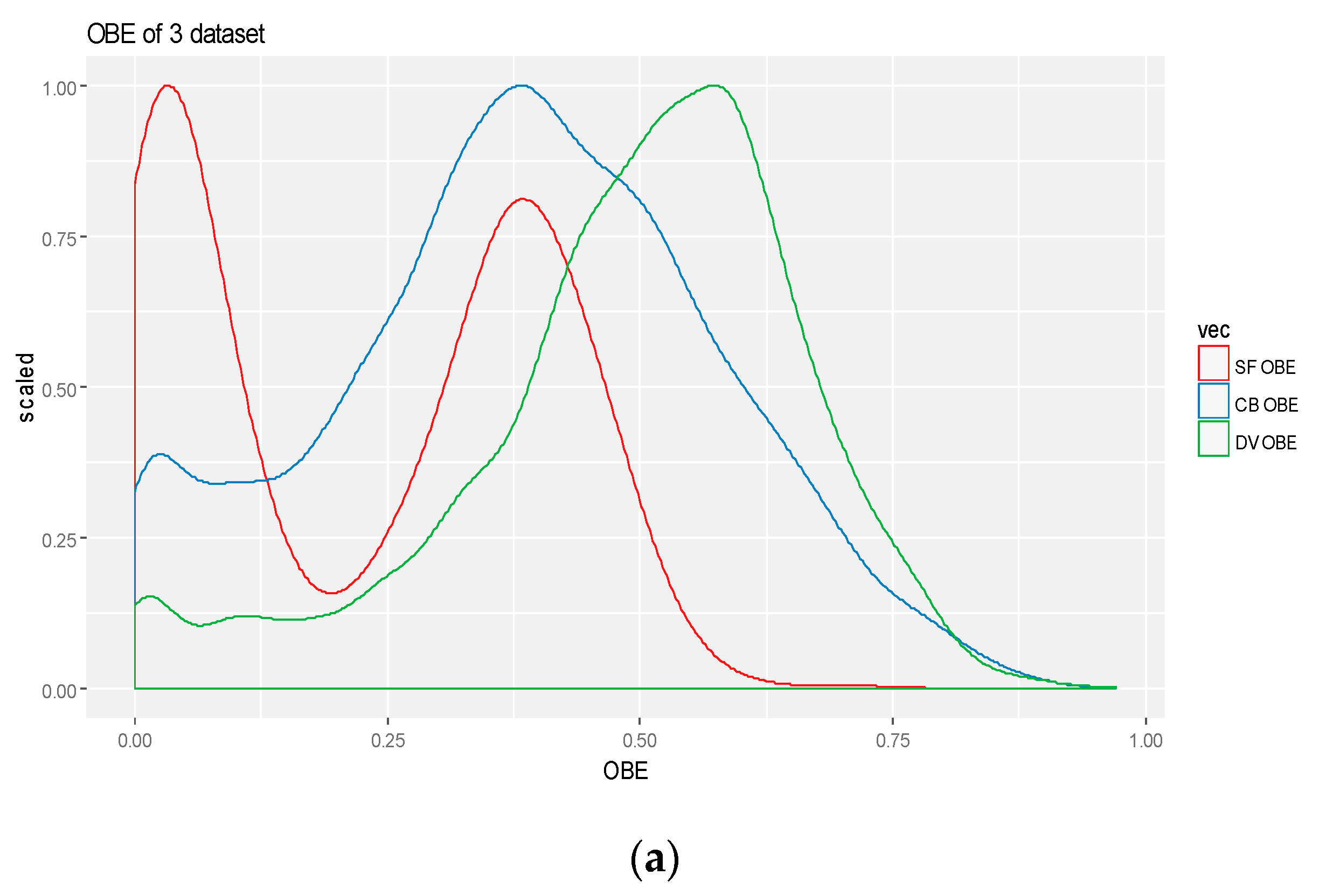
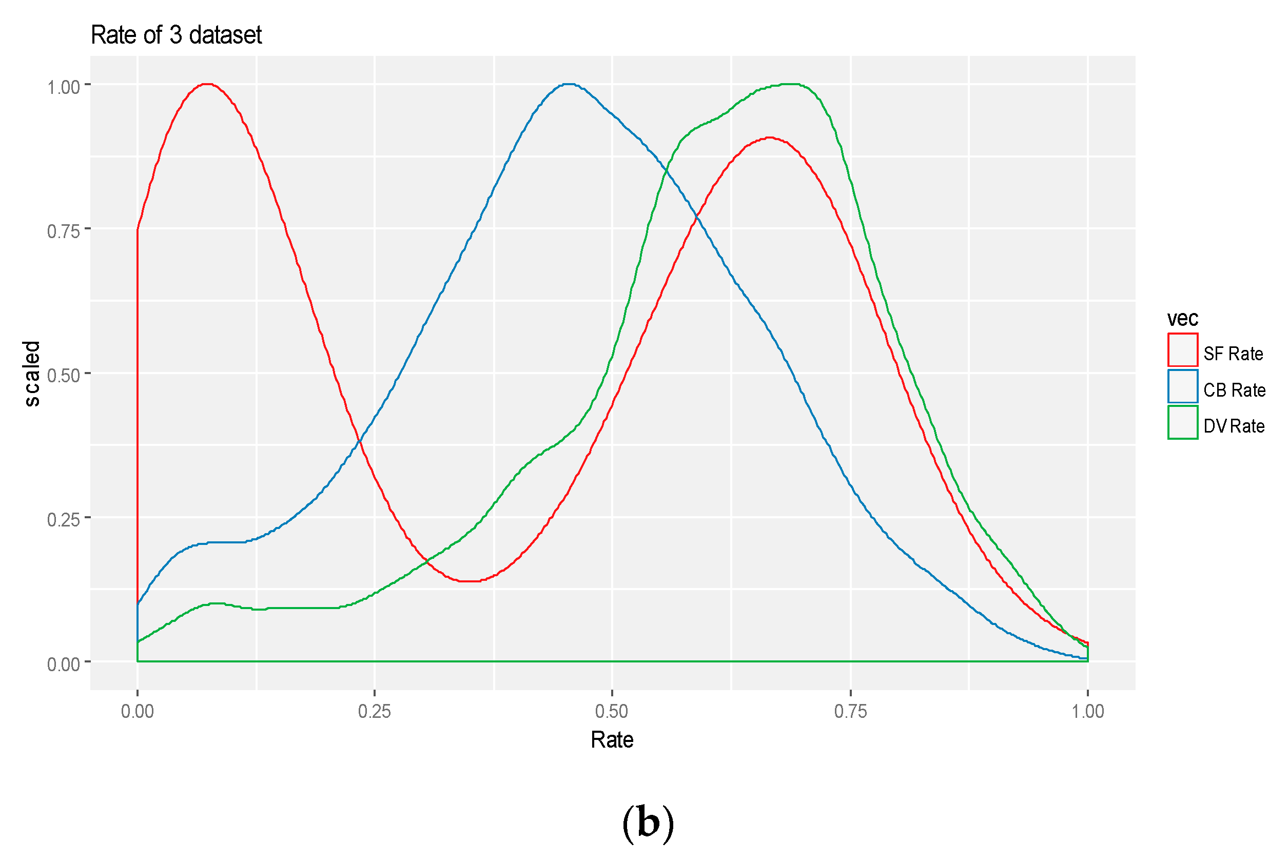
The existing frequency-based measures emphasize the actual trip frequency. In fact, BSS may vary according to the scheme scale such as density of population and the number of installed bikes. Therefore, the frequency-based measure often misleads the analysis when it is used as the benchmark measures. The OBE, on the other hand, underlines the use of time for the measures. The OBE result is a value scaled to the range in a closed interval [0, 1]. The same value type is also obtained using the Rate. The proportion values of both OBE and Rate are suitable to be used as measures for benchmarking. To show the applicability of the measures, this study applies three different datasets; the San Francisco Bay Area (SF), New York Citi Bike (CB) [53] and Chicago Divvy bikes (DV) [54]. One-month data, which is August 2014, is chosen from each dataset for the analysis. Note that August 2014 is chosen since the data had the highest actual trip frequency among other months in the same year.
The system information (# of installed bikes, # of (available) bikes, # of stations and population density) and measures comparison among the three different datasets are shown in Table 4. Note that the # of available bikes and the # of stations are obtained from the data instead of retrieved from the official site. The comparison took place among three measures; average trip per day, OBE and Rate. The average trip per day is derived from the actual trip frequency divided by the number of days in the respective month. The result of the average trip per day is incomparable due to the different number of bike installation. For example, CB dataset exhibits the superiority in terms of the number of trip since BSS of CB has the highest number of installed bikes among others. On the other hand, Rate and OBE are comparable. Table 4 shows that both Rate and OBE present DV as the BSS that has the highest values among the other two.
Figure 10a,b shows the density plot of three different datasets of OBE and Rate, respectively. The Rate measure seems to be higher than OBE since it considers only the frequency-based measure. Meanwhile, the OBE underlines the time aspect which results slightly difference in the data distributions. For example, using the Rate measure, SF and DV seem to have similar performance. Meanwhile, the OBE displays different distributions on those two datasets and illustrates a slightly similar distribution between SF and CB. From the graph, Rate seems to be more optimistic measure than OBE. As a matter of fact, the three BSS has begun their operation on about the mid of 2013. The early stage operation of the BSSs shows attractiveness (i.e., a trend) with less usage on the early periods [55]. Hence, OBE is a more realistic measure in comparison to Rate.
5.2. OBE for Life Cycle Analysis (Time to Time)
The frequency-based measures, such as the average trip per day and the number of daily trips, are the common measures to show the popularity of the BSS. Moreover, the accumulation of the trip frequency in a year, named as annual ridership, exhibits how the BSS improve annually. However, some issues occur when the measures are applied to explore the BSS life cycle. The actual trip frequency is a contrast with the number of available bikes. When a BSS has the same installed bikes in some consecutive years, there is a possibility of a decrement on the available bikes due to the maintenance issues such as damage. On the other hand, the performance of each bike may increase in the year later since the number of bikes is less than the year before.
Three datasets from a single BSS with a different period are used for the comparison of the measures; August 2014, August 2015 and August 2016. The system information (similarly as used in the previous section) as well as the performance measures (OBE, Rate and average trip per day (# of trip) are shown in Table 5. The table displays the comparison of SF BSS on the basis of year-over-year. Note that August is used for the experiment since the number of riders in August is the peak of other months in a year. According to the measures, the number of bikes used by riders is decreasing 5.4% from 628 in August 2014 to 594 in 2015 on the same month; and 3.3% from the year 2015 to 2016. Intuitively, the average trip per day will show an increment especially if the popularity increase. As a matter of fact, the average trip per day shows a slight decrement and Rate displays a stable value from 2015-08 to 2016-08, respectively. Since the average trip per day and Rate consider only the actual trip frequency, it fails to show the improvement of the BSS. On the other hand, the trend of OBE year-over-year intuitively displays the popularity of the BSS by considering the decrement of a number of bikes with the slight increment of the number of stations. Hence, the metric such as the number of trip and rate trip is not enough to represent the performance of the BSS.
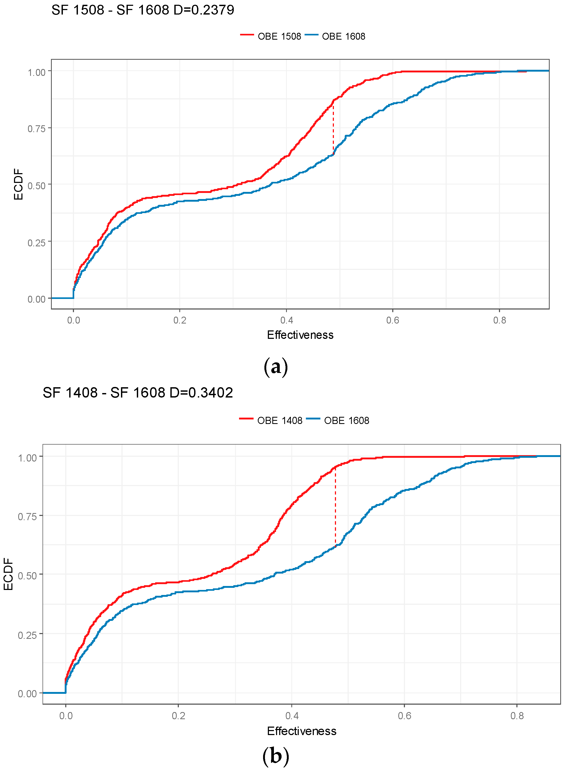
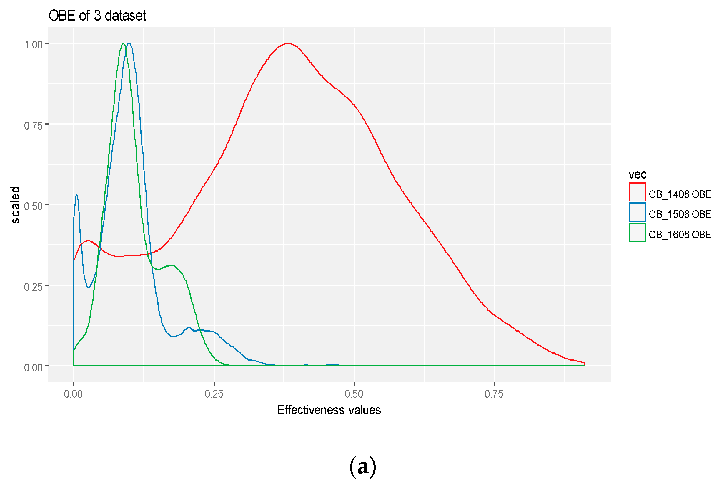
Figure 11a,b shows the density plot of three different datasets of OBE and Rate, respectively. The density plot among the measures could not clearly show the differences. Hence, K-S Test is performed to see whether there is an improvement on the system over the years. First, the K-S Test has been performed for year-over-year SF dataset. Figure 12 illustrates the K-S Test of OBE in two different years. The Figure 12a represents the K-S Test of OBE between SF 1508 and SF 1608. For comparison, the Figure 12b exhibits the K-S Test of OBE between SF 1408 and SF 1608. The result of δ value of the three datasets is shown in Table 6. The statistical analysis result shows each of the two different years has significant difference using 5% significance level with the table-based critical value 0.175. In summary, the OBE shows a different performance on year-over-year basis (from 2014 to 2016). As a result, OBE is able to show the life cycle of the BSS from time to time.
5.3. OBE for Evaluating the System Expansion
As aforementioned, the frequency-based measures are suitable to see the popularity of the BSS. When the BSS improves and expands the infrastructure such as increasing the number of installed bike and docking stations, some issues might occur. First, the frequency-based measures disregard the time utilization so that the effectiveness of BSS is unclear when the number of installed bikes is increasing. For example, the value of the average trip per day will decrease when the number of bikes increases. Second, the BSS expansion by establishing new docking stations will distribute the bikes in the diverse area. Accordingly, the number of trip will highly depend on the population density and the number of docks in the new station. Hence, frequency-based measures are unreliable to see the BSS performance. Instead, the use of time-based measures will lead toward performance assessment of the BSS after the system expansion. While the OBE could be used to show the life cycle analysis with the same number of installed bikes and docking stations, it could also present as a reliable evaluation measure when the resources expand.
The measures have been applied to CB as one of the BSS which expanded the resources in between 2014 and 2016. Some basic information, i.e., the number of installed bikes, was derived from the official BSS website [53]. Meanwhile, other basic information was obtained from the data. For the performance comparison, the previous three measures were used; OBE, Rate and average trip per day (# of trip). The detail system information and performance measurement are shown in Table 7. The number of bikes used by riders was increasing 31.43% from 5958 in 2014 to 7831 on the same month in 2015. Moreover, the number of the stations is also increasing 29.14% from 326 in 2014 to 421 in 2015. The average trip per day shows a decrement from 5.21 (2014) to 3.01 trips (2015) per day. The OBE also detects the same decrement as the average trip per day. However, the average trip per day in 2016 was decreasing compared to the previous year. Meanwhile, OBE and Rate shows an increment. The OBE shows a slight increment (from 0.10 (2015) to 0.11 (2016)) and Rate displays an increment which the value is almost the same as the year of 2014. In summary, the average trip per day shows a decrement value due to the increment of the number of installed bikes as well as the number of stations. However, Rate measure shows a contrast result in comparison to the other two measures. Intuitively, bike distribution to more stations could decrease the rate. Accordingly, the Rate increases while the average trip per day decreases. The inconsistency of frequency-based measure could not express the BSS performance. Hence, OBE offers a measure that considers the time to see the hidden performance during the operational time.
To clearly see the difference between frequency-based measure and time-based measure, the density plot is again performed. Figure 13a,b shows the density plot of three different datasets of OBE and Rate, respectively. It is clear that the performance of CB in August 2014 is the highest among the month in other years due to the smaller number of installed bikes compared to other years. In addition, OBE can clearly distinguish the performance of the three datasets in comparison to the Rate. Hence, OBE is useful to measure the BSS performance with regard to system expansion over years.
5.4. OBE as a Strategic Planning for Sustainability
The existing measures on BSS are limited to bike performance rather than strategic planning. In some cases, the existing type of BSS such as bike library system is undetectable using only frequency-based measures. The combination of both frequency- and time-based would enhance the analysis from the performance measurement into a strategic planning.
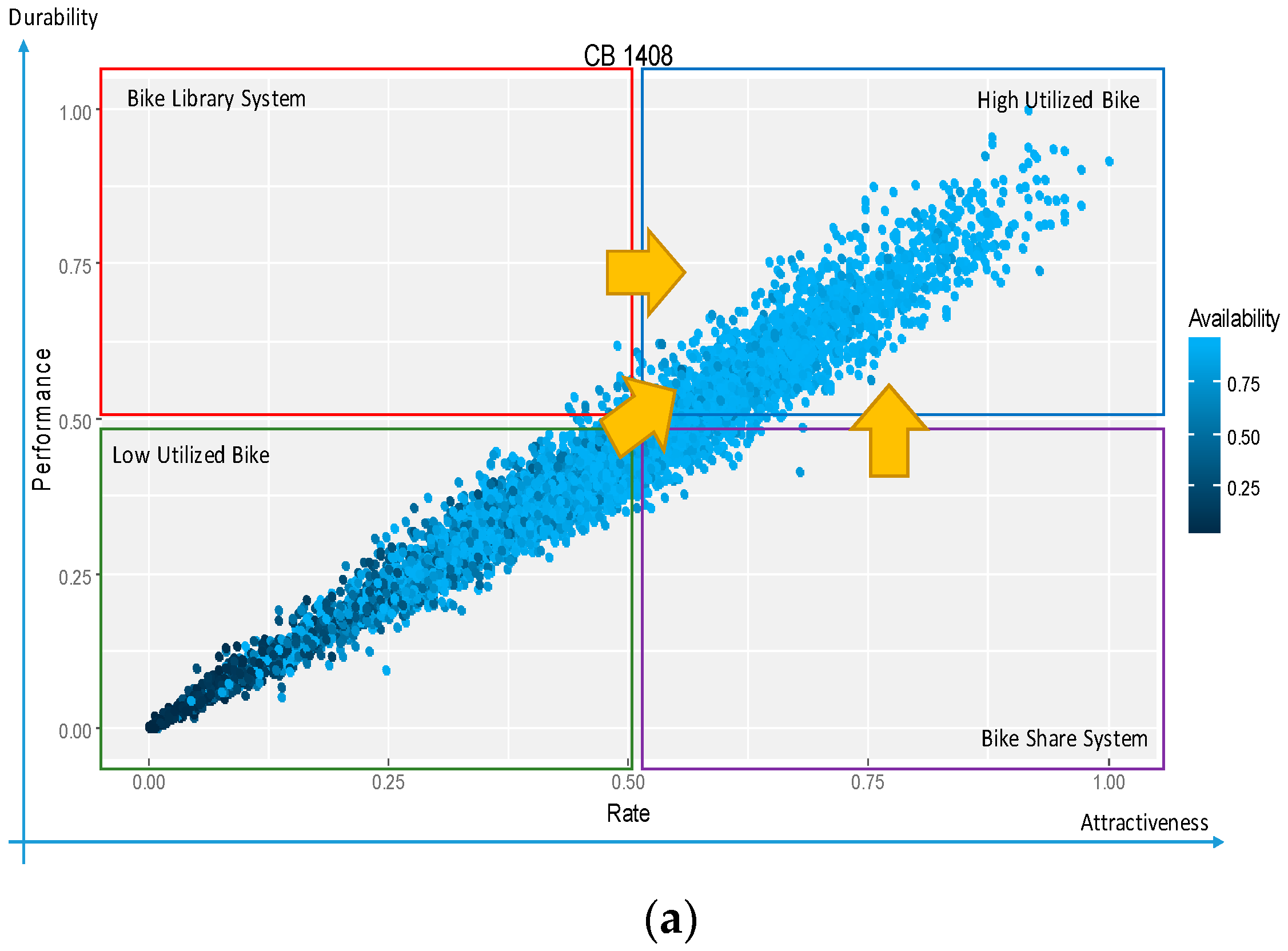
Using Performance and Rate (refers to the dot plot in Figure 5), the two aspects, durability and attractiveness, can be disaggregated into four categories of bike utilization; Bike Library System (BLS), BSS, High Utilized Bike and Low Utilized Bike (refers to Figure 14). It is necessary to pay more attention to the two quadrants; low utilized bike with the low-frequency trip and low utilized bike with the high-frequency trip. Low-frequency trip commonly expresses as a bike with the low utility trip. Meanwhile, a low utilized bike with high-frequency trip refers to BLS. BLS, as aforementioned, is one of a particular category of BSS that has a different purpose from BSS. While BSS is a high-frequency and short trip system, BLS shows a type of low frequency and long trip system.
The empirical analysis on SF dataset (using the data on September 2014) results in a dot plot as shown in Figure 14. Low utilized bikes are highly available. To accommodate low utilized bike with high availability, some promotional strategies are necessary. Assuming that increasing the number of trips will reduce the average operating cost per trip, the promotional trip is somewhat effective for travelers or customer. For example, a service provider could give a free rent cost to the traveler who rides the bike in particular national day or event.
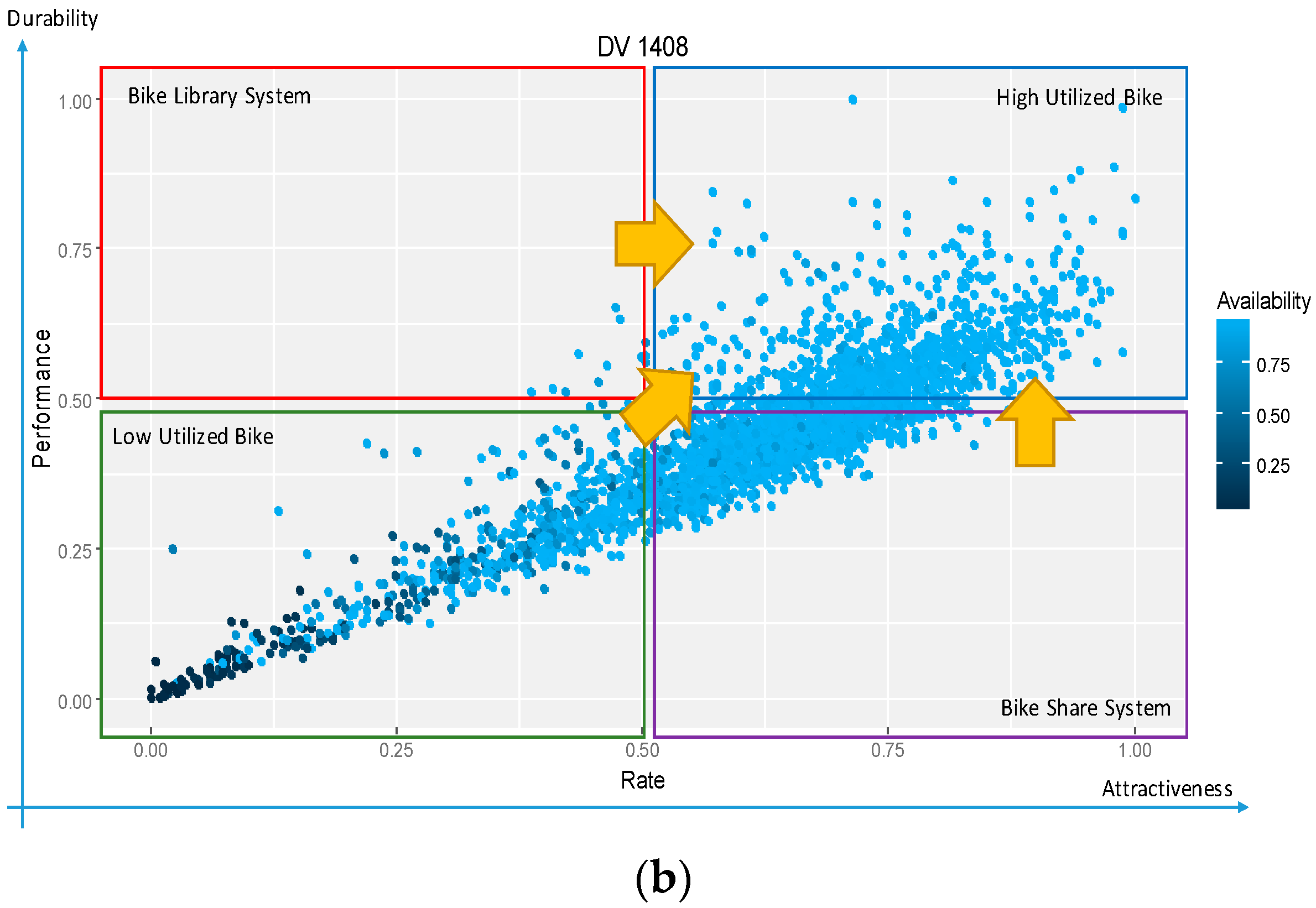
Figure 15a,b illustrates the analysis using the dot plot for CB and DV dataset, respectively. Based on the graph, the BSS of CB performs with balance measures of Performance and Rate. In other word, the value of Rate is linearly dependent on the Performance. For example, high-frequency trip bikes have high utilizations. In addition, high Rate and high Performance resemble high availability. In contrast, DV shows slightly lower in Performance compared to CB but higher than the Performance of SF. Hence, based on the Performance and Rate measures, the operator of both CB and DV could focus on improving the utilization of bikes. Infrastructure improvement effort could be an option to enhance the bike utilization. For example, establishing more stations may increase the bike utilizations in term of Performance.
6. Conclusions
This study proposed a sustainability metric, called OBE, to evaluate the effectiveness of bikes as well as the BSS. Many studies have been done on sustainable bike sharing systems. However, the operational view, as one of the aspects influencing the sustainability of a system, had been neglected. The negligence of bike performance based on the operational view will not only affect the bike effectiveness but also implicate the overall BSS. BSS, as a PSS, is expressed in different types of service and behaviors to clarify the loss and drive effective improvements for the system design when establishing a new BSS in similar regions. OBE indices are expressed with bike trip and thus different types of bike performance loss can be identified in a comprehensive framework to clarify the need of maintenance and/or replacement from operators, third-party entities to drive effective improvements for bike availability, bike performance and bike quality. Critical issues and improvement directions can be accurately recognized via the proposed measures for maximizing overall bike effectiveness in regard to the operational aspects. The theoretical-OBE are also proposed to address the BSS effectiveness at the early stage of implementations.
Furthermore, the proposed metric has several value propositions. First, the metric can be employed for best practice benchmarking among BSS and thus adopts some improvement directions to reduce particular loss. Second, it is also useful as time-to-time analysis for a particular BSS with similar system properties such as the same number of installed bikes and the same number of docking stations over the year. Third, system expansion could be assessed using the metric to indicate the potential improvement of the BSS with different system properties such as an increment of the number of installed bikes and a new establishment of docking stations. Finally, the OBE can be used as a strategic planning for BSS sustainability. Toward the sustainability, the OBE could also be seen in the four different quadrants; Low Utilized Bike, High Utilized Bike, Bike Library System and Bike Share System. Low utility bikes with low and high-frequency trips would be the concerns quadrant for improvement. Applying promotional efforts and infrastructure efforts would boost the effectiveness of the BSS.
Although the analysis result shows the usefulness of the proposed metric, there are some limitation issues. First, time-based measure considers only general time instead of particular time such as business time or event time. For example, time-related events, such as holidays and festivals, in the region could affect the increment of the number of trips. In addition, the ineffective trip time is measured only based on the ineffective loop trip. Other ineffective trip such as damage in bicycle after a period higher than the operator threshold is not considered due to data limitation. Second, the metric utilizes only time while three pillars of sustainability such as economic, social and environmental perspective are neglected due to data limitation. Third, the metric excludes docking stations as one of the BSS properties.
There are at least three potential issues for future work. First, the proposed OBE metric can be integrated with other attributes such as the type of riders and the effectivity of stations as weighted OBE to address multiple operations and business objectives, referring to the three pillars of sustainability; economic, social and environment. Second, determining best practices of BSS could assist new regions which are willing to establish the similar program and enhance the existing BSS toward sustainable BSS. As BSS reached the third phase with a technology-based system such as GPS-based and other related IoT, there is a need to select some role models for other regions. Indeed, the best practices of particular BSS would be utilized as an input for the success of the cities to implement the similar system. Finally, the proposed OBE can be employed as a support measure for operators’ process improvement. Bike reallocation and replacement are the two operational issues for the operators. By measuring the OBE, operators can decide the route to reallocate and replace bikes for meeting riders’ demand.
Conflicts of Interest
The author declares no conflict of interest.
Notation
| Notation | Description |
| O | Operational Time |
| TT | Trip Time |
| ETTk | Effective Trip Time of k-th bike |
| Ak | Availability of k-th bike |
| Average of the availability of all bikes | |
| Pk | Performance of k-th bike |
| Average of the performance of all bikes | |
| Qk | Quality of k-th bike |
| Average of the quality of all bikes | |
| ATk | The active time of k-th bike |
| TTTbest | The best total trip time |
| TTTk | Total trip time of k-th bike |
| ILTk | Ineffective loop trip of k-th bike |
| LUTk | Low utility trip of k-th bike |
| ETTk | Effective Trip Time of k-th bike |
| ITTk | Ineffective Trip Time of k-th bike |
| TOBE | Theoretical OBE |
| TA | Theoretical Bike Availability |
| TP | Theoretical Bike Performance |
| TQ | Theoretical Bike Quality |
| R | Rate |
| ST | Start Time |
| ET | End Time |
| D | Duration |
| SS | Start Station |
| ES | End Station |
| S | A set of station (S ⊆ SS ⋃ ES) |
| U | Rider’s type (customer, subscriber) |
| TTF | Target trip frequency |
References
- DeMaio, P. Smart bikes: Public transportation for the 21st century. Transp. Q. 2003, 57, 9–11. [Google Scholar]
- Larsen, J. Bike-Sharing Programs Hit the Streets in over 500 Cities Worldwide; Earth Policy Institute: Washington, DC, USA, 2013. [Google Scholar]
- Shaheen, S.A. Public Bikesharing in North America during a Period of Rapid Expansion: Understanding Business Models, Industry Trends and User Impacts; Mineta Transportation Institute (MTI): San Jose, CA, USA, 2015. [Google Scholar]
- Fishman, E. Bikeshare: A review of recent literature. Transp. Rev. 2016, 36, 92–113. [Google Scholar] [CrossRef]
- Low, N.; Gleeson, B.; Green, R.; Radovic, D. The Green City: Sustainable Homes, Sustainable Suburbs; Routledge, Taylor & Francis Group: Sydney, Australia, 2005. [Google Scholar]
- Zhang, L.; Zhang, J.; Duan, Z.-Y.; Bryde, D. Sustainable bike-sharing systems: Characteristics and commonalities across cases in urban China. J. Clean. Prod. 2015, 97, 124–133. [Google Scholar] [CrossRef]
- Schieferdecker, A. Pedal talk the fall and rise of bikes and bike sharing in the twin cities. Cities 21st Century 2013, 3. Available online: http://digitalcommons.macalester.edu/cgi/viewcontent.cgi?article=1024&context=cities (accessed on 1 September 2017).
- Fishman, E.; Washington, S.; Haworth, N.; Mazzei, A. Barriers to bikesharing: An analysis from Melbourne and Brisbane. J. Transp. Geogr. 2014, 41, 325–337. [Google Scholar] [CrossRef]
- DeMaio, P. Bike-sharing: History, impacts, models of provision and future. J. Public Transp. 2009, 12, 41–56. [Google Scholar] [CrossRef]
- Bike-share Returns to Helsinki in 2016. Available online: http://yle.fi/uutiset/osasto/news/bike-share_returns_to_helsinki_in_2016/8385342 (accessed on 20 August 2017).
- Today, A. 2016 Bike Share Season Coming to a Close. Available online: http://today.anl.gov/2016/11/2016-bike-share-season-coming-to-a-close/ (accessed on 20 August 2017).
- Fishman, E.; Washington, S.; Haworth, N. Bike share: A synthesis of the literature. Transp. Rev. 2013, 33, 148–165. [Google Scholar] [CrossRef] [Green Version]
- Hawkins, A.J. Citi bike turnaround: So much promise, so many problems. Crain’s New York Business, 26 April 2015. [Google Scholar]
- Colville-Andersen, M. Watching Copenhagen Bike Share Die. Available online: http://www.copenhagenize.com/2015/02/watching-copenhagen-bike-share-die.html (accessed on 20 August 2017).
- Gauthier, A.; Hughes, C.; Kost, C.; Li, S.; Linke, C.; Lotshaw, S.; Mason, J.; Pardo, C.; Rasore, C.; Schroeder, B.; et al. The Bike-Share Planning Guide; Institute for Transportation & Development Policy: New York, NY, USA, 2014. [Google Scholar]
- Pater, L.R.; Cristea, S.L. Systemic definitions of sustainability, durability and longevity. Procedia Soc. Behav. Sci. 2016, 221, 362–371. [Google Scholar] [CrossRef]
- Williamson, M.W. Measuring the Sustainability of U.S. Public Bicycle Systems; University of New Orleans: New Orleans, LA, USA, 2012. [Google Scholar]
- Buehler, R.; Pucher, J. Cycling to sustainability in Amsterdam. Sustain Fall/Winter 2010, 21, 36–40. [Google Scholar]
- Deffner, J.; Ziel, T.; Hefter, T.; Rudolph, C. Handbook on Cycling Inclusive Planning and Promotion: Capacity Development Material for the Multiplier Training within the Mobile2020 Project. Available online: http://www.mobile2020.eu/fileadmin/Handbook/M2020_Handbook_EN.pdf (accessed on 1 September 2017).
- Büttner, J.; Mlasowsky, H.; Birkholz, T.; Gröper, D.; Fernández, A.C.; Emberger, G.; Petersen, T.; Robèrt, M.; Vila, S.S.; Reth, P.; et al. Optimising Bike Sharing in European Cities: A Handbook. Available online: https://www.carplusbikeplus.org.uk/wp-content/uploads/2015/09/Obis-Handbook.pdf (accessed on 1 September 2017).
- Zhang, Y.; Zuidgeest, M.; Brussel, M.; Sliuzas, R.; Maarseveen, M.V. Spatial Location-Allocation Modeling of Bike Sharing Systems: A Literature Search. In Proceedings of the 13th World Conference on Transport Research, Rio de Janeiro, Brazil, 15–18 July 2013; pp. 1–14. [Google Scholar]
- Singhvi, D.; Singhvi, S.; Frazier, P.I.; Henderson, S.G.; Mahony, E.O.; Shmoys, D.B.; Woodard, D.B. Predicting Bike Usage for New York City’s Bike Sharing System; Association for the Advancement of Artificial Intelligence: Palo Alto, CA, USA, 2015. [Google Scholar]
- Transportation Service; Commuter Service. Bicycle Rack Utilization Study & Bicycle Facilities Improvement Report; University of Washington: Seattle, WA, USA, 2008. [Google Scholar]
- Li, J.; Ren, C.; Shao, B.; Wang, Q.; He, M.; Dong, J.; Chu, F. A solution for reallocating public bike among bike stations. In Proceedings of the 9th IEEE International Conference on Networking, Sensing and Control (ICNSC), Beijing, China, 11–14 April 2012. [Google Scholar]
- Chemla, D.; Meunier, F.; Calvo, R.W. Bike sharing systems: Solving the static rebalancing problem. Discret. Optimiz. 2013, 10, 120–146. [Google Scholar] [CrossRef] [Green Version]
- Kaltenbrunner, A.; Meza, R.; Grivolla, J.; Codina, J.; Banchs, R. Urban cycles and mobility patterns: Exploring and predicting trends in a bicycle-based public transport system. Pervasive Mob. Comput. 2010, 6, 455–466. [Google Scholar] [CrossRef]
- Jensen, P.; Rouquier, J.-B.; Ovtracht, N.; Robardet, C. Characterizing the speed and paths of shared bicycle use in lyon. Transp. Res. Part D Transp. Environ. 2010, 15, 522–524. [Google Scholar] [CrossRef]
- Sayarshad, H.; Tavassoli, S.; Zhao, F. A multi-periodic optimization formulation for bike planning and bike utilization. Appl. Math. Model. 2012, 36, 4944–4951. [Google Scholar] [CrossRef]
- Nakajima, S. Introduction to TPM Total Productive Maintenance; Productivity Pr: Cambridge, MA, USA, 1988. [Google Scholar]
- Nakajima, S. TPM Development Program: Implementing Total Productive Maintenance; Massachusetts Productivity Press: Cambridge, MA, USA, 1989. [Google Scholar]
- Borkowski, S.; Czajkowska, A.; Stasiak-Betlejewska, R.; Borade, A.B. Application of TPM indicators for analyzing work time of machines used in the pressure die casting. J. Ind. Eng. Int. 2014, 10, 1–9. [Google Scholar] [CrossRef]
- Zairi, M. Business process management: A boundaryless approach to modern competitiveness. Bus. Process Manag. J. 1997, 3, 64–80. [Google Scholar] [CrossRef]
- Pintelon, L.M.-Y.A.; Muchiri, P.N. Performance measurement using overall equipment effectiveness (OEE): Literature review and practical application discussion. Int. J. Prod. Res. 2010, 46, 3517–3535. [Google Scholar]
- Puvanasvaran, A.P.; Mei, C.Z.; Alagendran, V.A. Overall equipment efficiency improvement using time study in an aerospace industry. Procedia Eng. 2013, 68, 271–277. [Google Scholar] [CrossRef]
- Samat, H.A.; Kamaruddin, S.; Azid, I.A. Integration of overall equipment effectiveness (OEE) and reliability method for measuring machine effectiveness. S. Afr. J. Ind. Eng. 2012, 23, 92–113. [Google Scholar]
- SEMI E124-1107—Guide for Definition and Calculation of Overall Factory Efficiency (OFE) and Other Associated Factory-Level Productivity Metrics; SEMI: Mountain View, CA, USA, 2007.
- Chien, C.-F.; Hu, C.-H.; Hu, Y.-F. Overall space effectiveness (OSE) for enhancing fab space productivity. IEEE Trans. Semicond. Manuf. 2016, 29, 239–247. [Google Scholar] [CrossRef]
- Kronos. Overall Labor Effectiveness (OLE): Achieving a Highly Effective Workforce; Kronos: Chelmsford, MA, USA, 2007. [Google Scholar]
- Chien, C.-F.; Chen, H.-K.; Wu, J.-Z.; Hu, C.-H. Constructing the OGE for promoting tool group productivity in semiconductor manufacturing. Int. J. Prod. Res. 2007, 45, 509–524. [Google Scholar] [CrossRef]
- Muthiah, K.M.N.; Huang, S.H. Overall throughput effectiveness (OTE) metric for factory-level performance monitoring and bottleneck detection. Int. J. Prod. Res. 2006, 45, 4753–4769. [Google Scholar] [CrossRef]
- Chien, C.-F.; Hsu, C.-Y.; Chang, K.-H. Overall wafer effectiveness (OWE): A novel industry standard for semiconductor ecosystem as a whole. Comput. Ind. Eng. 2013, 65, 117–127. [Google Scholar] [CrossRef]
- Voehl, F.; Harrington, H.J.; Mignosa, C.; Charron, R. The Lean Six Sigma Black Belt Handbook—Tools and Methods for Process Acceleration; CRC Press: Boca Raton, FL, USA, 2014. [Google Scholar]
- Dalmolen, S.; Moonen, H.; Iankoulova, I.; Hillegersberg, J.V. Transportation performances measures and metrics: Overall transportation effectiveness (OTE): A framework, prototype and case study. In Proceedings of the 46th Hawaii International Conference on System Sciences, Maui, HI, USA, 7–10 January 2013. [Google Scholar]
- Berhan, E. Overall service effectiveness on urban public transport system in the city of Addis Ababa. Br. J. Appl. Sci. Technol. 2016, 12, 1–9. [Google Scholar] [CrossRef]
- Personal Transit System in Phoenix, Mesa & Tempe. Available online: http://gridbikes.com/ (accessed on 26 October 2017).
- Taipei Ubike Official Website. Available online: http://taipei.youbike.com.tw/en/ (accessed on 26 October 2017).
- OBIS Consortium. Obis—European Bike Sharing Scheme on Trial. In Optimising Bike Sharing in European Cities: A Handbook; European Commission/European Union: Brussels, Belgium, 2011; Chapter 3; Available online: https://www.carplusbikeplus.org.uk/wp-content/uploads/2015/09/Obis-Handbook.pdf (accessed on 1 September 2017).
- Keeling, B. San Francisco Named Second Most Bike Friendly City in the U.S. Available online: https://sf.curbed.com/2016/9/19/12982284/sf-bike-friendly-city-cycling (accessed on 18 April 2017).
- Bay Area Bike Share Open Data. Available online: http://www.bayareabikeshare.com/open-data (accessed on 18 April 2017).
- Ford Go Bike. Available online: https://www.fordgobike.com/ (accessed on 20 September 2017).
- Bay Area Bike Share Data Challenge. 2014. Available online: http://www.bayareabikeshare.com/datachallenge-2014 (accessed on 18 April 2017).
- Sahoo, P. Probability and Mathematical Statistics; University of Louisville: Louisville, KY, USA, 2013. [Google Scholar]
- Citi Bike Nyc. Available online: https://www.citibikenyc.com (accessed on 20 September 2017).
- Divvy Bike Dataset. Available online: https://www.divvybikes.com/system-data (accessed on 20 September 2017).
- Divvy: Chicago’s Newest Transit System. Available online: http://divvybikes.tumblr.com/post/96460660270/new-divvy-data-now-available (accessed on 26 October 2017).
Figure 1.
Models of Provision [9].
Figure 1.
Models of Provision [9].

Figure 2.
OBE Framework.

Figure 3.
(a) Events of bike #1 and (b) events of bike #5 over the time.
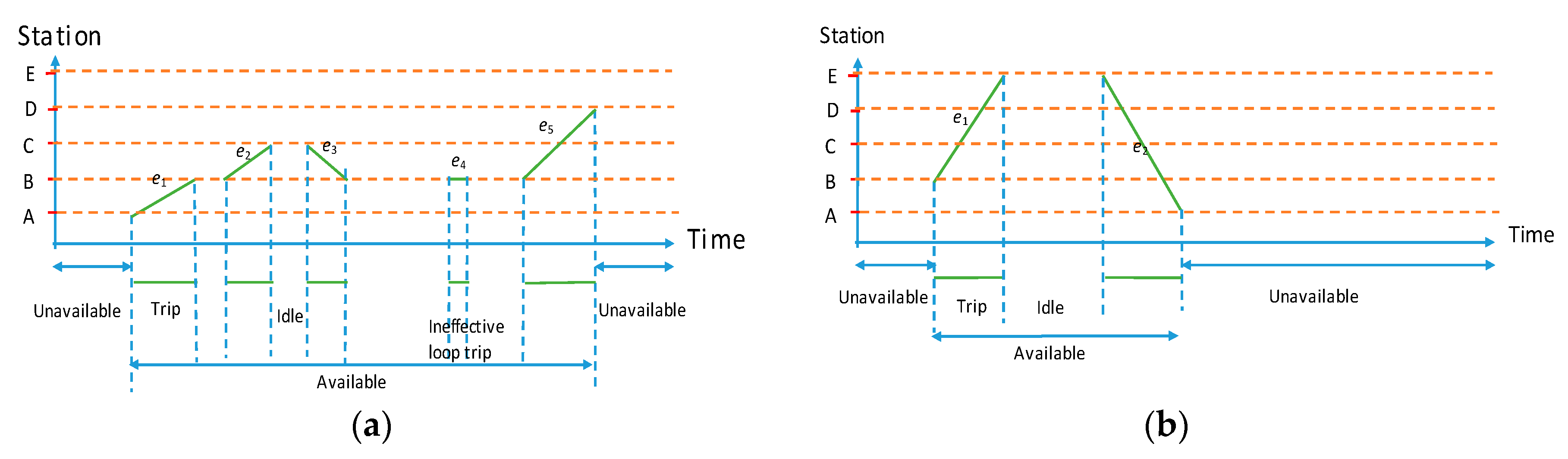
Figure 4.
(a) Dotted plot of trip event and (b) Scatter plot of duration.


Figure 5.
Dot plot of Performance and Rate of SF dataset.
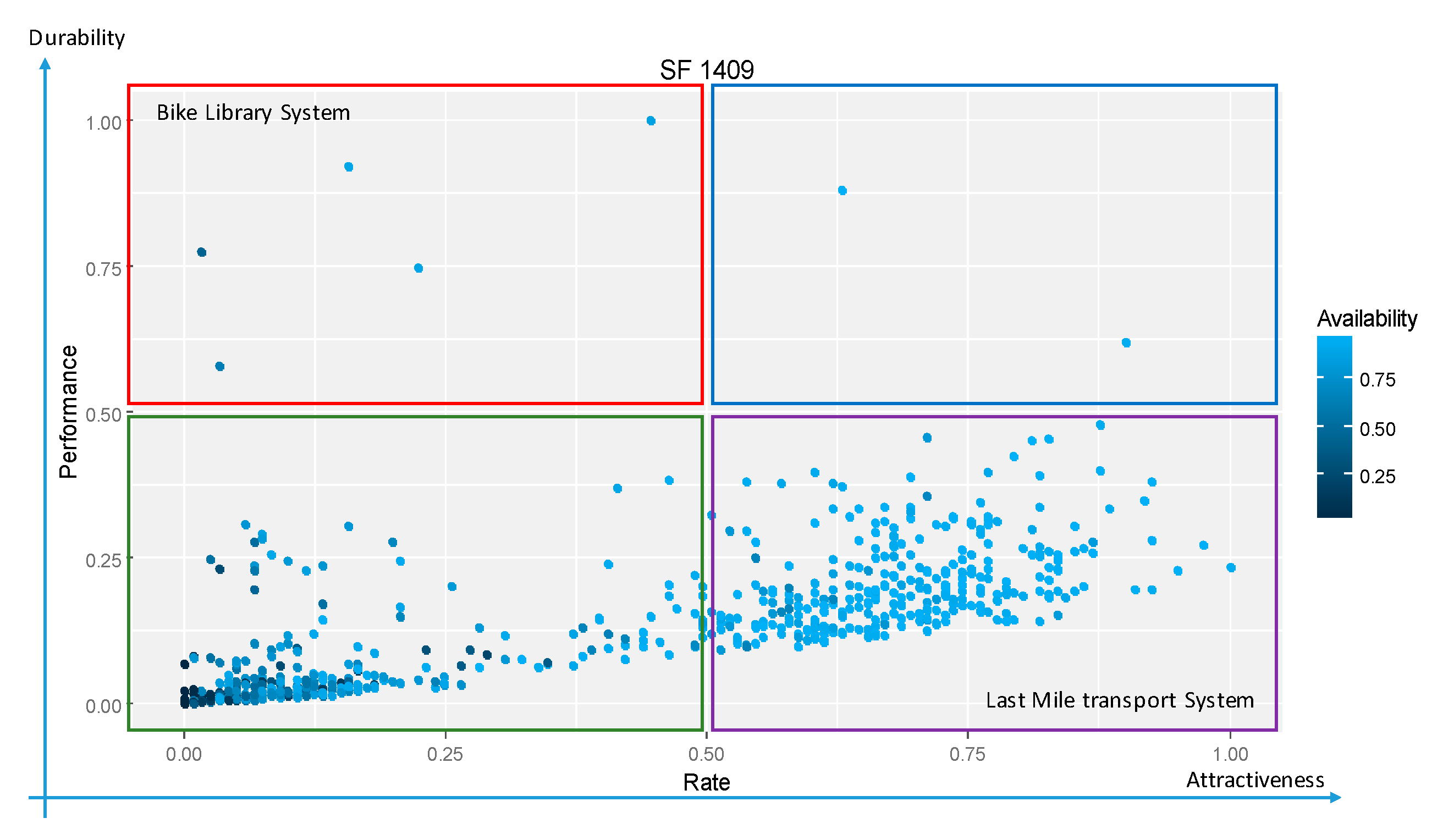
Figure 6.
Correlation plot among factors of OBE.
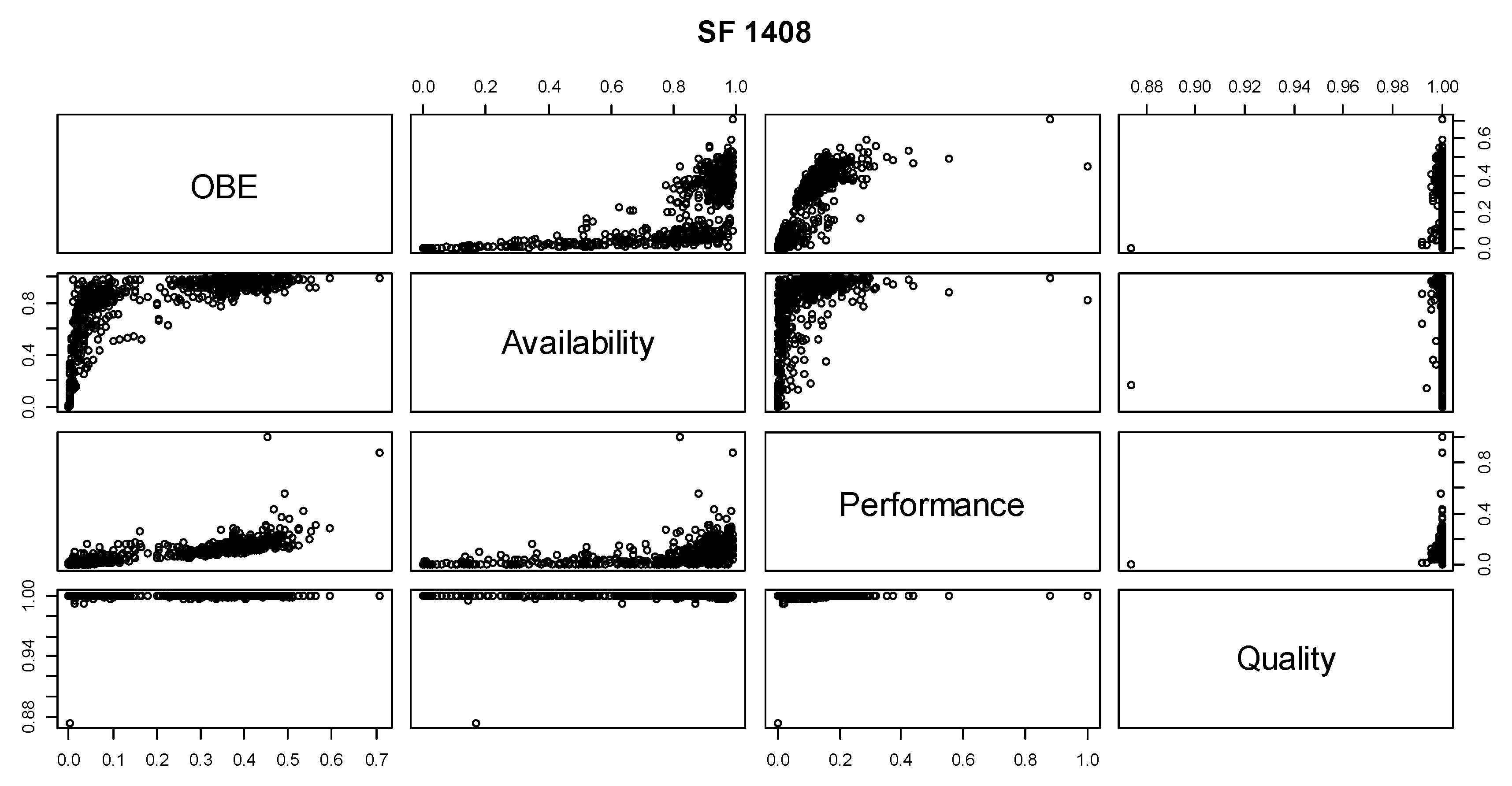
Figure 7.
Density plot of OBE variables.
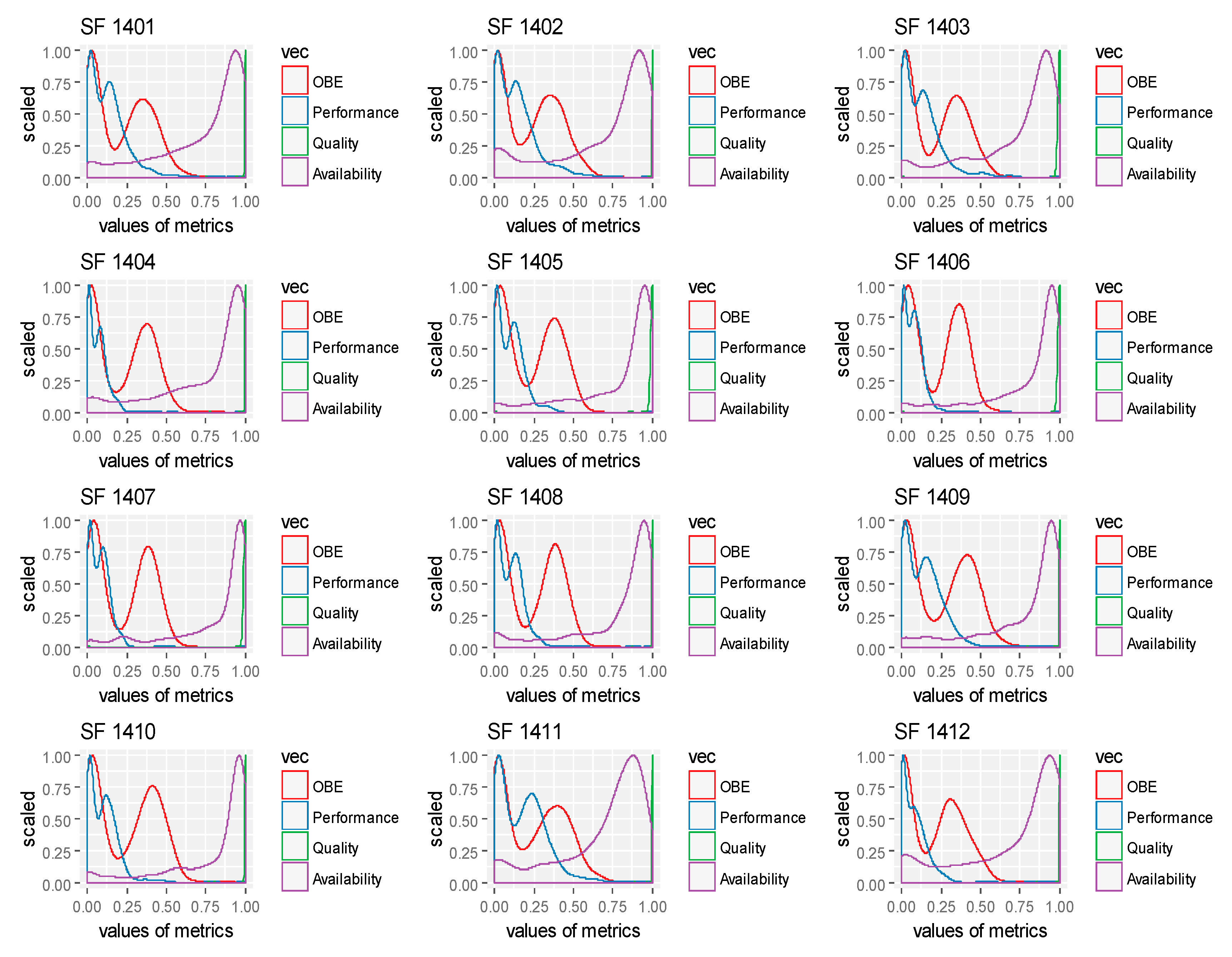
Figure 8.
Density plot of OBE and Rate.

Figure 9.
Kolmogorov Smirnov Test between OBE and Rate of SF Data in November 2014.

Figure 10.
Density plot of (a) OBE and (b) Rate of three different datasets.


Figure 11.
Density plot of (a) OBE and (b) Rate of three different years (August of 2014, 2015, 2016) of SF dataset.
Figure 11.
Density plot of (a) OBE and (b) Rate of three different years (August of 2014, 2015, 2016) of SF dataset.
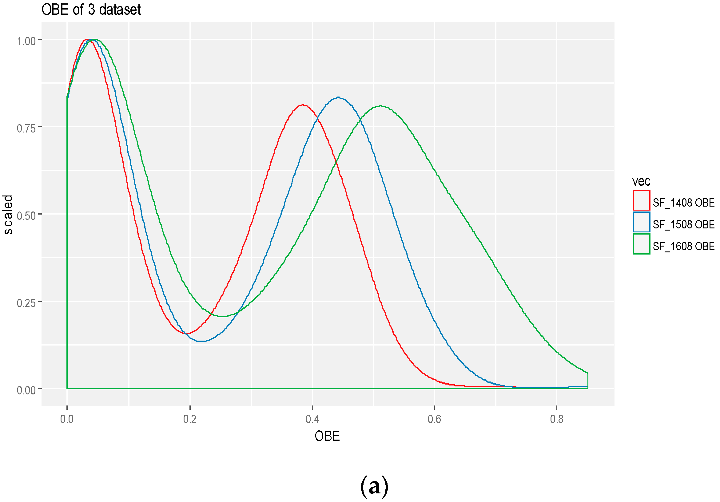
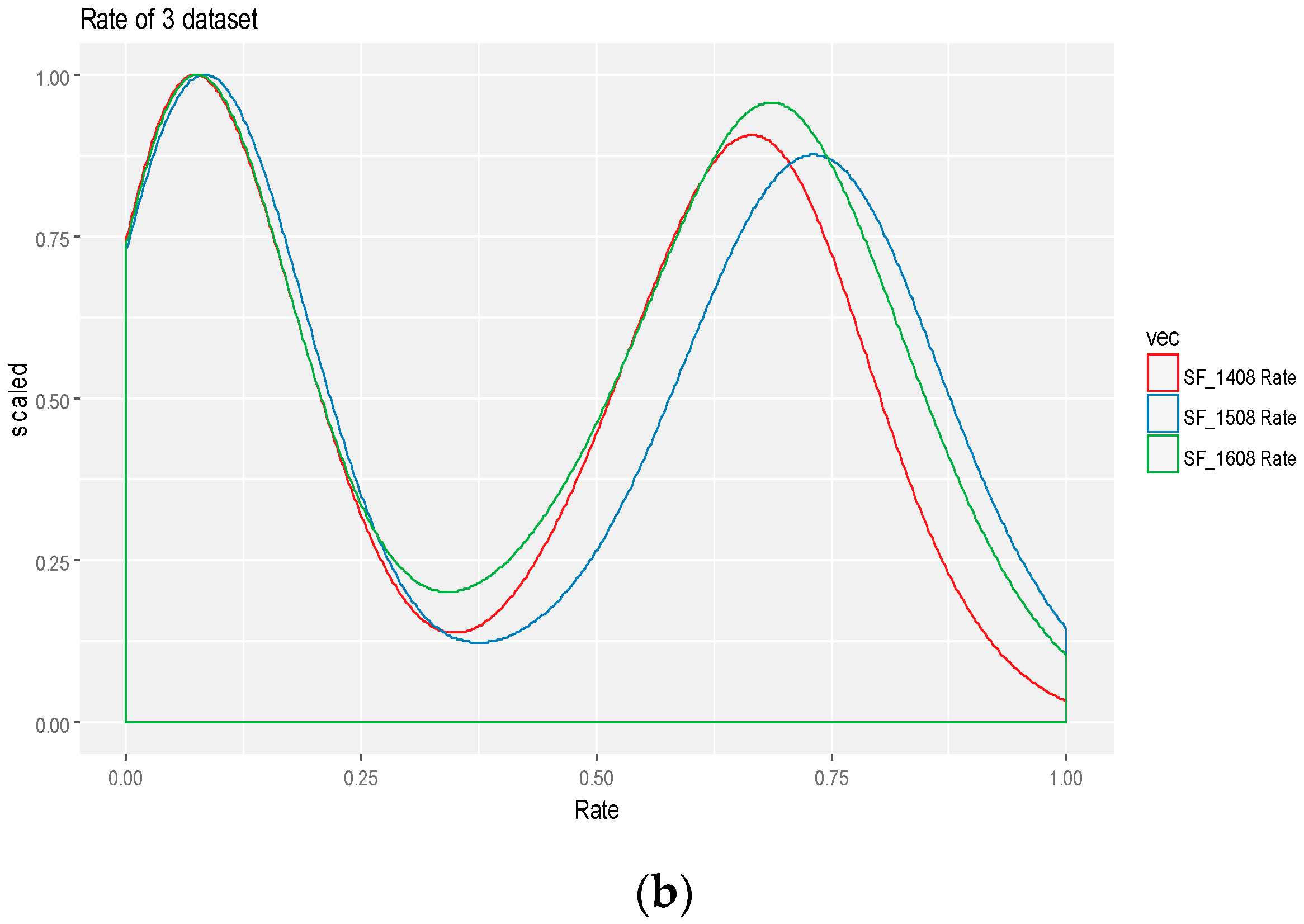
Figure 12.
K-S Test for the dataset SF for two samples (a) 1508–1608 and (b) 1408–1608.

Figure 13.
Density plot of (a) OBE and (b) Rate of three different years of CB dataset with different number of bike installation (5958, 7831 and 5650, respectively).
Figure 13.
Density plot of (a) OBE and (b) Rate of three different years of CB dataset with different number of bike installation (5958, 7831 and 5650, respectively).

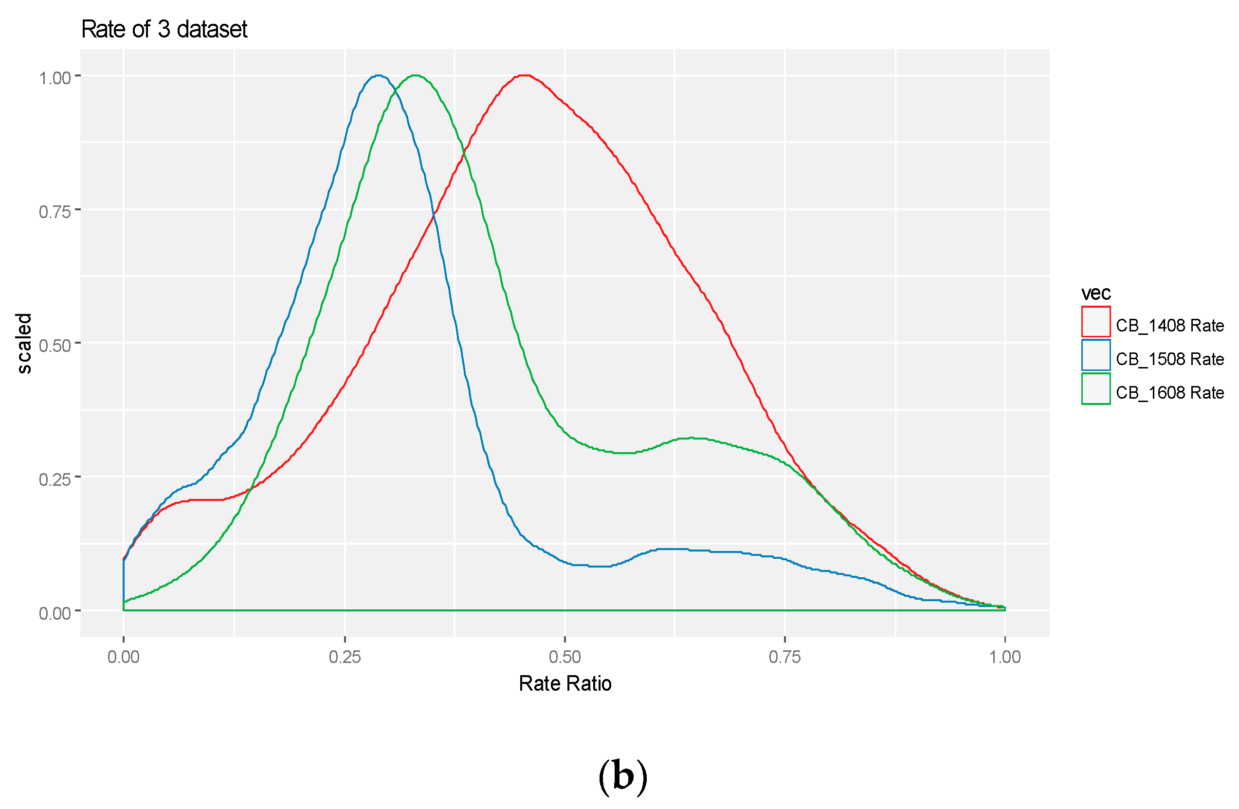
Figure 14.
Categorization of bike utilization according to performance and frequency rate of SF 1409 dataset.
Figure 14.
Categorization of bike utilization according to performance and frequency rate of SF 1409 dataset.
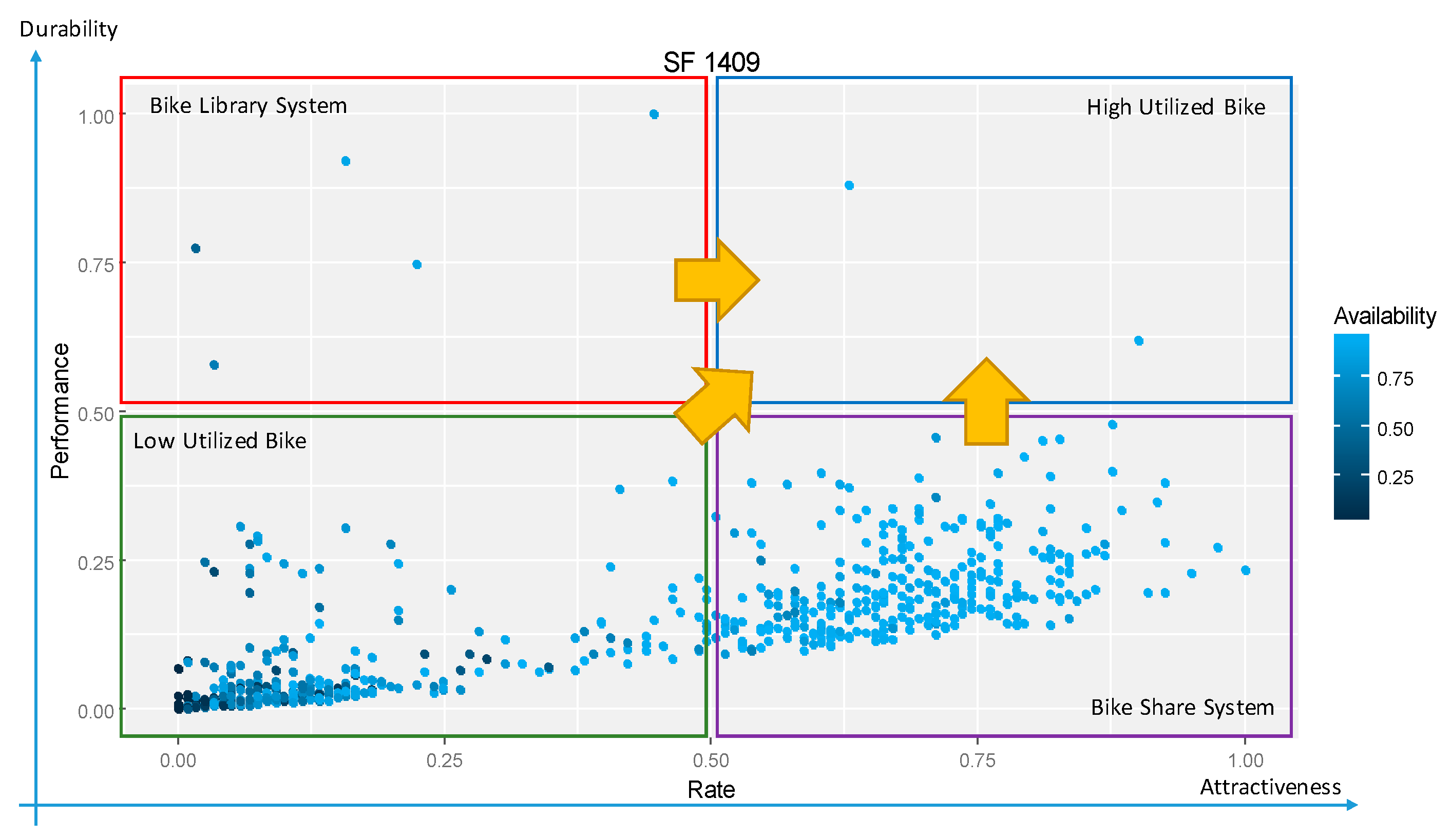
Figure 15.
Dot plot of performance and rate of (a) CB 1408 and (b) DV 1408.


Table 1.
Fragment of bike trip data.
| Bike ID | Start Trip | End Trip | Duration (s) | Origin Station | Destination Station | User |
|---|---|---|---|---|---|---|
| 1 | 2015-02-24 11:24:00 | 2015-02-24 11:31:00 | 425 | A | B | Subscriber |
| 1 | 2015-02-24 11:45:00 | 2015-02-24 11:49:00 | 247 | B | C | Customer |
| 1 | 2015-02-24 23:54:00 | 2015-02-24 23:59:00 | 271 | C | B | Subscriber |
| 1 | 2015-02-26 08:13:00 | 2015-02-26 08:15:00 | 118 | B | B | Customer |
| 1 | 2015-02-26 22:36:00 | 2015-02-26 22:51:00 | 935 | B | D | Customer |
| 2 | 2015-02-24 06:47:00 | 2015-02-24 07:07:00 | 1164 | B | E | Subscriber |
| 2 | 2015-02-26 18:06:00 | 2015-02-26 18:16:00 | 595 | E | C | Customer |
| 2 | 2015-02-26 19:43:00 | 2015-02-26 19:49:00 | 314 | C | D | Subscriber |
| 2 | 2015-02-26 22:07:00 | 2015-02-26 22:13:00 | 378 | D | B | Customer |
| 3 | 2015-02-24 09:02:00 | 2015-02-24 09:08:00 | 365 | C | B | Customer |
| 3 | 2015-02-24 18:29:00 | 2015-02-24 18:37:00 | 461 | B | D | Subscriber |
| 3 | 2015-02-24 20:32:00 | 2015-02-24 20:50:00 | 1108 | D | E | Customer |
| 3 | 2015-02-25 13:45:00 | 2015-02-25 14:15:00 | 1828 | E | D | Subscriber |
| 3 | 2015-02-25 19:54:00 | 2015-02-25 19:56:00 | 158 | D | A | Customer |
| 3 | 2015-02-26 11:38:00 | 2015-02-26 11:46:00 | 456 | A | B | Customer |
| 3 | 2015-02-26 12:16:00 | 2015-02-26 12:23:00 | 433 | B | C | Subscriber |
| 3 | 2015-02-26 18:09:00 | 2015-02-26 18:26:00 | 970 | C | B | Subscriber |
| 4 | 2015-02-25 09:52:00 | 2015-02-25 10:02:00 | 589 | B | D | Subscriber |
| 5 | 2015-02-24 18:59:00 | 2015-02-24 19:02:00 | 147 | B | E | Subscriber |
| 5 | 2015-02-25 07:56:00 | 2015-02-25 07:59:00 | 140 | E | A | Subscriber |
| 6 | 2015-02-24 08:55:00 | 2015-02-24 12:58:00 | 14,580 | A | E | Customer |
| 7 | 2015-02-24 13:29:00 | 2015-02-24 13:30:00 | 99 | E | E | Customer |
| 7 | 2015-02-26 16:47:00 | 2015-02-26 16:49:00 | 95 | E | C | Customer |
| 7 | 2015-02-26 17:20:00 | 2015-02-26 17:26:00 | 352 | C | B | Customer |
Table 2.
Time derivation for effectiveness calculations.
| Bike ID | Available Time (min) | Total Trip Time (s) | Ik | LUTk | ILTk | Ak (%) | Pk (%) | Qk (%) | OBEk (%) |
|---|---|---|---|---|---|---|---|---|---|
| 1 | 3567 | 1996 | 5 | 0 | 118 | 82.56 | 13.68 | 94.08 | 10.62 |
| 2 | 3806 | 2451 | 4 | 0 | 0 | 88.10 | 16.81 | 100.0 | 14.80 |
| 3 | 3444 | 5779 | 8 | 0 | 0 | 79.72 | 39.63 | 100.0 | 31.56 |
| 4 | 10 | 589 | 1 | 589 | 0 | 0.23 | 4.03 | 0 | 0 |
| 5 | 780 | 287 | 2 | 287 | 0 | 18.05 | 1.97 | 0 | 0 |
| 6 | 243 | 14,580 | 1 | 0 | 0 | 5.63 | 100.00 | 100.0 | 5.63 |
| 7 | 3117 | 546 | 3 | 546 | 0 | 72.15 | 3.74 | 0 | 0 |
| Average | 2138.14 | 3743 | 3.43 | 203.14 | 16.85 | 49.49 | 25.69 | 56.29 | 8.94 |
Table 3.
K-S test using 5% significance level with the critical value of 0.175.
| Dataset | δ | Dataset | δ |
|---|---|---|---|
| SF 1401 | 0.3768 | SF 1407 | 0.4596 |
| SF 1402 | 0.4046 | SF 1408 | 0.4697 |
| SF 1403 | 0.4136 | SF 1409 | 0.4236 |
| SF 1404 | 0.4709 | SF 1410 | 0.4456 |
| SF 1405 | 0.4496 | SF 1411 | 0.3679 |
| SF 1406 | 0.4773 | SF 1412 | 0.4104 |
Table 4.
Comparison among BSS on the same time basis.
| Dataset | Population Density | # of Installed Bikes | # of Bikes | # of Stations | OBE | # of Trip | Rate |
|---|---|---|---|---|---|---|---|
| SF 1408 | 1.2 | 700 | 628 | 74 | 0.23 | 1.66 | 0.39 |
| CB 1408 | 1.2 | 7000 | 5958 | 326 | 0.38 | 5.21 | 0.46 |
| DV 1408 | 2.1 | 5800 | 2770 | 300 | 0.49 | 4.71 | 0.60 |
Table 5.
Comparison of SF Bay Share BSS annually (August).
| Dataset | # of Installed Bikes | # of Bikes | # of Stations | OBE | # of Trip | Rate |
|---|---|---|---|---|---|---|
| SF 1408 | 700 | 628 | 74 | 0.23 | 1.66 | 0.39 |
| SF 1508 | 700 | 594 | 75 | 0.26 | 1.79 | 0.43 |
| SF 1608 | 700 | 574 | 75 | 0.32 | 1.76 | 0.43 |
Table 6.
Two sample K-S Test result between two datasets.
| Dataset1–Dataset2 | δ |
|---|---|
| SF 1408–SF 1508 | 0.1794 |
| SF 1508–SF 1608 | 0.2379 |
| SF 1408–SF 1608 | 0.3402 |
Table 7.
Citi Bike BSS from 2014 to 2016.
| Year-Month | # of Installed Bikes | # of Bikes | # of Stations | OBE | # of Trip | Rate |
|---|---|---|---|---|---|---|
| CB 1408 | 7000 | 5958 | 326 | 0.38 | 5.21 | 0.46 |
| CB 1508 | 10,000 | 7831 | 421 | 0.10 | 3.01 | 0.31 |
| CB 1608 | 10,000 | 5650 | 580 | 0.11 | 2.95 | 0.42 |
© 2017 by the author. Licensee MDPI, Basel, Switzerland. This article is an open access article distributed under the terms and conditions of the Creative Commons Attribution (CC BY) license (http://creativecommons.org/licenses/by/4.0/).
Share and Cite
MDPI and ACS Style
Yahya, B.N. Overall Bike Effectiveness as a Sustainability Metric for Bike Sharing Systems. Sustainability 2017, 9, 2070. https://doi.org/10.3390/su9112070
AMA Style
Yahya BN. Overall Bike Effectiveness as a Sustainability Metric for Bike Sharing Systems. Sustainability. 2017; 9(11):2070. https://doi.org/10.3390/su9112070
Chicago/Turabian StyleYahya, Bernardo Nugroho. 2017. "Overall Bike Effectiveness as a Sustainability Metric for Bike Sharing Systems" Sustainability 9, no. 11: 2070. https://doi.org/10.3390/su9112070
Note that from the first issue of 2016, this journal uses article numbers instead of page numbers. See further details here.