All articles published by MDPI are made immediately available worldwide under an open access license. No special
permission is required to reuse all or part of the article published by MDPI, including figures and tables. For
articles published under an open access Creative Common CC BY license, any part of the article may be reused without
permission provided that the original article is clearly cited. For more information, please refer to
https://www.mdpi.com/openaccess.
Feature papers represent the most advanced research with significant potential for high impact in the field. A Feature
Paper should be a substantial original Article that involves several techniques or approaches, provides an outlook for
future research directions and describes possible research applications.
Feature papers are submitted upon individual invitation or recommendation by the scientific editors and must receive
positive feedback from the reviewers.
Editor’s Choice articles are based on recommendations by the scientific editors of MDPI journals from around the world.
Editors select a small number of articles recently published in the journal that they believe will be particularly
interesting to readers, or important in the respective research area. The aim is to provide a snapshot of some of the
most exciting work published in the various research areas of the journal.
Analysis of Interval Data Envelopment Efficiency Model Considering Different Distribution Characteristics—Based on Environmental Performance Evaluation of the Manufacturing Industry
Collaborative Innovation Center on Forecast and Evaluation of Meteorological Disasters, School of Economics and Management, China Institute for Manufacture Developing, Nanjing University of Information Science and Technology, Nanjing 210044, China
*
Author to whom correspondence should be addressed.
This study utilizes the Data Envelopment Efficiency (DEA) model to assess input–output efficiency from two perspectives. First, not considering the distribution of interval data, we introduce an adjusted parameter to transform interval data to determination data. Second, by contrast, we take into account the distribution characteristics of interval data and test the DEA model with interval data based on linear uniform distribution and normal distribution with uncertainty. Based on the normal distribution DEA evaluation model, this paper aims to evaluate the input–output performance of the manufacturing industry with the constraint of environmental pollution in the Yangtze River Delta (YRD) region, China. Research has shown that the optimal solution of the normal distribution model is better than that of linear distribution. Therefore, it is imperative to adopt an appropriate method to evaluate the energy and environmental efficiency of this region.
To maintain sustainable economic development, China is now subject to a number of crucial constraints, including but not limited to: the outstanding supply–demand discrepancies in energy, severe environmental pollution, and regional discrepancies in energy efficiency. Enhancing energy efficiency and environmental efficiency is an important way to confront energy crisis and to prevent environmental pollution, and, ultimately, to boost China’s sustainable development capability and to promote economic restructuring. The Yangtze River Delta agglomeration is one of the regions with the highest level of economic development in China. The heightened levels of industrialization, urbanization and energy consumption have led to the dramatic decline in energy supply and the deterioration of environmental quality. Drawing upon an investigation on the energy efficiency with the environmental constraints of the Yangtze River Delta region, we explore the causes of low energy efficiency and seek practical recommendations to improve energy efficiency in order to alleviate some of the pressure on energy consumption. Many authors think it is useful to explain the productivity efficiency of Chinese manufacturing sectors using DEA [1,2,3,4]. Hence, the efficiency evaluation method of data envelopment analysis (DEA) is used to explore the energy efficiency differences of 16 cities in the Yangtze River Delta region from 2005 to 2014 under the environmental constraints.
Data envelopment analysis (DEA) was originally proposed by Charnes [5] and is a system analysis method based on “relative efficiency”. As a non-parametric evaluation method of the DEA model, the project efficiency evaluation problem with single-input and single-output gradually expanded into a complex system evaluation problem with multi-inputs and multi-outputs, which is widely used in many fields, such as mathematical economics and operations research. If the input–output data of decision-making units (DMUs) in the DEA model are accurate, the DEA method belongs to the definite type of DEA. However, in practice, due to measurement errors and data noise, amongst other reasons, the evaluation indicator values of each DMU often cannot be accurately determined, so the CCR [6,7,8], BCC [9,10,11], SBM [12], SBI DEA [13,14] and TurboDEA [15] models were derived.
Furthermore, in practice, problems such as policy strength assessment and investment projects evaluation arise and some or even all of the input–output indicators of DMUs can only be uncertain values due to the qualitative policy strength and uncertainty of economic phenomena. To overcome the limitations of the traditional DEA method, many authors have expanded to the random DEA [16,17], interval DEA [18,19,20,21] and normal DEA models [22,23,24], amongst others, which are mainly used to solve the problem relating to the DEA model with uncertain values.
(1) When the input and output variables are denoted as stochastic, the corresponding DEA model is known as the stochastic DEA model. The distribution of the input–output variables includes logarithmic normal, exponential and normal distributions. Cooper et al. [25] supposed that the variable obeys logarithmic normal distribution and as there was no abnormal variable, and the original addition model was converted to the multiplication model for efficiency solution. The study of the stochastic DEA model with logarithmic normal distribution also includes [26,27,28,29,30,31]. Zhang [32] further proposed a chance constraint to the stochastic DEA model based on exponential distribution, since input–output indicators obeyed the same distribution, and analyzed the effectiveness of corresponding DMUs in theory. The stochastic DEA model of exponential distribution also includes [33,34,35,36]. Jeang [37] assumed that the stochastic variables in the chance constraint model obeyed normal distribution. Consequently, the nonlinear stochastic DEA model was applied to solve the maximum output scale by using computer software (such as computer-aided engineering and DEA software).
(2) Under normal conditions, the stochastic DEA model is frequently solved by the stochastic simulation method. The concept of the satisfaction degree was introduced into the stochastic DEA problem and the consensus DEA model was proposed, e.g., by [38,39,40,41,42,43]. Furthermore, the confidence region or level was introduced into the stochastic DEA model, e.g., by [44,45,46,47,48]. The Monte Carlo simulation algorithm was used to solve the problem of stochastic input and output variables and the study of stochastic DEA is one of the directions of current research, such as studies by [49,50,51,52,53,54]. The stochastic DEA model including the Bayesian method, such as in studies by [55,56,57,58,59,60], was used to deduce the efficiency value of a finite sample.
(3) For special stochastic DEA models, the isometric transformation method is an effective method for solving the stochastic DEA model. Khodabakhshi and Asgharian [61] constructed a general deterministic stochastic DEA model that can replace the nonlinear model under normal conditions. Eslami et al. [62] dealt with a real decision problem with fuzzy constraints and uncertain information (stochastic data). The fuzzy probability constraint in the uncertain constraint DEA model was transformed into the equivalent form of certainty. Zhou et al. [63] took advantage of chance-constrained programming, the key value reduction method and equivalent transformation to solve stochastic uncertain problems and to measure the effectiveness, efficiency and productivity in uncertain environments and for different confidence levels. Yu et al. [64] combined time series and regression methods to construct a new stochastic chance constrained model and used it to evaluate and analyze the efficiency of 15 commercial banks from 2005 to 2011.
This study utilizes DEA model to assess input–output efficiency from two perspectives. First, not considering the distribution of interval data, we introduce an adjusted parameter to transform interval data to determination data. Second, by contrast, we take into account the distribution characteristics of interval data and test the DEA model with interval data based on linear uniform distribution and normal distribution with uncertainty. Research has shown that the optimal solution of the normal distribution model is better than that of linear distribution. Based on the normal distribution DEA evaluation model, this paper aims to evaluate the input–output performance of the manufacturing industry with the constraint of environmental pollution in the YRD region, China.
In practical efficiency evaluation, interval input–output variables often exist. In conventional interval DEA model processing, the efficiency solution of the DMUs is restricted by the interval endpoint values (upper and lower limits) if only the intervals are considered. In this study, we investigate the relative effectiveness of DMUs with different distributions, based on two cases of intervals obeying linear and normal distribution, respectively.
2. Preliminaries and Methodology
2.1. Standard DEA Model with Crisp Data
Supposing that there are n DMUs , m types of different resources invested and s kinds of different outputs yielded, input–output vectors of would be denoted separately as follows:
For , compared to other DMUs in efficiency solving, the traditional CCR model is constructed as follows [5]:
where and are the weight coefficients of outputs and inputs, respectively, and their values are not negative. The objective function is the maximum efficiency for , and is evaluated DMU in this model. is reference target for non-efficient DMU [65].
In Model (1), to keep the input unchanged and maximize the output, we construct a linear programming Model (2) as follows:
Constraint (2-1) represents the unchanged input of the DMUs and the objective function is to maximize the output of the , is evaluated DMU in this model.
The duality of linear programming can be denoted by the real variable and the non-negative vector [66]. To avoid the weakly efficient problem with a non-zero slack variable, we add the constraint of the sum of the maximum slack variables in the objective function. In this paper, Model (2) is transformed into Model (3) as follows:
is evaluated DMU in this model. and are introduced as slack variables in the model and the selection of slack variables do not affect the value of the optimal solution . With the same output, the objective function of the dual model is to find the difference between the minimum variable elasticity and the slack variable. If and all the slack variables are zero, i.e., and , then it is absolutely efficient. If and all the slack variables are not zero, i.e., or , then the DMUs are weakly efficient.
In Model (3), the constraint is added and the model could subsequently be transformed into the following BCC model:
is evaluated DMU in this model. Constraint (4-3) represents the variable scale returns, i.e., the ratio of the output increment of the DMUs is not equal to that of the increment of the input factor.
2.2. Interval DEA model
In Model (4), the input and output indicators are all accurate numbers. In practice, the input and output indicators may be intervals, and DEA Model (5) based on the interval indicators is constructed as follows:
In Model (5), the input–output indicators, ; , are interval data, is evaluated DMU in this model.
From the perspective of optimization, we first transform the input and output interval into an accurate number to obtain the optimal solution for Model (5). That is, let , , , and , respectively. The interval DEA model could be transformed into the conventional accurate DEA Model (6) as follows:
is evaluated DMU in this model.
2.2.1. Examples of Interval DEA Model
There were six DMUs and the input indicator , and output indicators and are intervals (Table 1).
Taking the input–output data in Table 1 as the example data, which are similar to those in the traditional Model (2), the interval DEA nonlinear model is constructed as follows:
is evaluated DMU in this model. Let , for , so ; and let , for , so .
The nonlinear interval DEA Model (7) is transformed into a linear Model (8) as follows:
is evaluated DMU in this model.
According to the dual equivalence principle, the linear interval DEA Model (8) is transformed into a dual linear Model (9) as follows:
Yagi et al. [67] regard the variables of the above model as shadow price, is efficient when the profit of shadow price equals zero. is evaluated DMU in this model. We use Lingo 11 software (LINDO SYSTEMS Inc., Chicago, IL, USA) to solve the aforementioned model and the optimal solution is shown in Table 2.
From Table 2, are not efficient, whereas are efficient; the efficiency from to therefore increases. In the next section, we discuss the improvement of the non-efficient DMUs in the DEA model.
2.2.2. The Improvement of the Non-Efficient DMU
Definition1.
The DEA’s relative efficiency (efficient production frontier) is . If the is DEA efficient, and the optimal solution of linear programming (P) satisfies the condition
Furthermore, , so . Therefore, the point is on the hyper plane π and the other points on the hyper plane π are also DEA efficient. Therefore, we use the method of “projection” on the relative efficient surface to improve the DMUs that were non-efficient for DEA.
Definition2.
Assume that are the optimal solution to the duality of linear programming, and let
We call of the projection of the corresponding on the DEA relative efficient surface π.
Non-efficient could be constructed into a new , as seen in Table 3.
The dual nonlinear Model (10) of a new interval DEA is constructed as follows:
is evaluated DMU in this model. is evaluated DMU in this model. If the efficiency of is 1, then the new is efficient and could be constructed in accordance with the data of new DMU. Similarly, other non-efficient DMUs could be changed into new DMUs, as shown in Table 4.
2.3. Uncertain DEA Model
There are disordered, probable, vague and approximate attributes, i.e., uncertainty in the process of contact and development of objective things. Therefore, Liu [68] introduced the uncertainty theory mainly to solve decision-making optimization under the uncertain information environment. It is a mathematical theory concerning the quantitative characteristics of various uncertain phenomena.
In this section, the input–output objectives , are assumed separately to obey the uncertain linear distribution (as seen in Section 2.1) and the uncertainty of the normal distribution (as seen in Theorem 1 in Supplementary Materials).
Based on the dual Model (3), we construct the unchanged inputs, maximum outputs and opportunity constraint DEA Model (11) as follows:
is evaluated DMU in this model, where is a non-Archimedes infinitesimally small constant, namely , and M is the uncertainty measure. Model (11-1) shows that the probability of occurrence of expected outputs of the DMUs being larger than the actual outputs is , which improves the expected outputs. Model (11-2) shows that when ’s outputs remain unchanged, we should assure that the input values decrease as the same ratio , i.e., the probability of occurrence of expected inputs being less than the actual investment is and the corresponding adjustments are made to the DMUs that are deficient compared to DMUs that are efficient for DEA.
The objective function can be seen as having two parts, one of which is to minimize the real number of the linear programming dual model and the other is to maximize the value of the total slack variables in the input–output constraint. Assuming that the optimal problem is given by Model (11), we obtained the optimal solution that . Furthermore, there is and . We subsequently call the evaluation DMU is efficient compared to other DMUs and satisfied both the technical and scale effectiveness. If , but or are not equal to the zero vector at the same time, then we call that the DMUs are weakly efficient and the DMUs are not technically and scale efficient at the same time. If , then the DMUs are evaluated as DEA non-efficient.
2.3.1. Uncertain DEA Model Based on Linear Distribution
Definition3.
Assume that an uncertain variable ξ obeys the linear uncertainty distribution as follows:
Consequently, obeys the linear probability distribution, where a and b are definite numbers and . Then, we call ξ obeys the linearly uniform distribution of , expressed as .
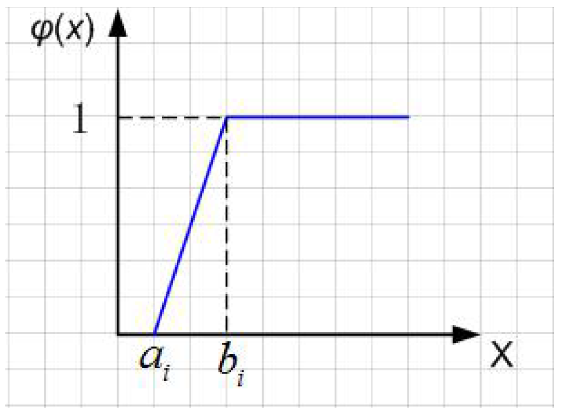
Definition4.
Let ξ be the uncertain variable obeying the linear uncertainty distribution (Figure 1). The inverse function is called the inverse uncertain distribution function of an uncertain variable . The inverse uncertain distribution function of linear uncertain distribution is as follows:
Based on the certain input and the largest output background, the uncertain DEA model based on linear distribution is constructed as follows:
According to Definition 5, Model (12) is transformed into a deterministic DEA Model (13).
Definition5.
Uncertain linear distribution of DEA Model (12) with chance constraints is equivalent to the determined DEA Model (13):
is evaluated DMU in this model. As and increases, the objective function is an increasing function of the probability and , and the objective function becomes larger. Similarly, if increases, the objective function also becomes larger.
2.3.2. A Numerical Example of Uncertain Linear Distribution DEA Model Based on Opportunity Constraint
Assuming that there are still six DMUs for the interval model, the input indicators , and the output indicators and are the interval data in Table 1, which are subjected to linear uncertain distribution. The data can be seen in Table 5.
2.4. A Numerical Example of Equivalent DEA Nonlinear Transformation Model for Uncertainty Distribution
The input and output interval data (Table 5) indicators of the DMUs subjected to linear distribution are taken as the numerical example. We construct the equivalent nonlinear DEA Model (14) from the linear distribution model, which is similar to the certain linear distribution DEA Model (13):
is evaluated DMU in this model.The parameter “ ”is the representation of shadow price.
2.4.1. A Linear Equivalent Model for Nonlinear DEA Transformation Model
Let , for , so ; and let , for , so .
The linear equivalent Model (15) of the nonlinear DEA transformation model is as follows:
is evaluated DMU in this model. Model (15) is solved by Lingo 11 software and the optimal solution is shown in Table 6.
As seen from Table 6, are not efficient and the efficiency is lower than that of the original interval model (compared with those in Table 2). The efficiencies of to present an increasing trend.
2.4.2. The Concept of Normal Uncertainty Distribution
Definition6.
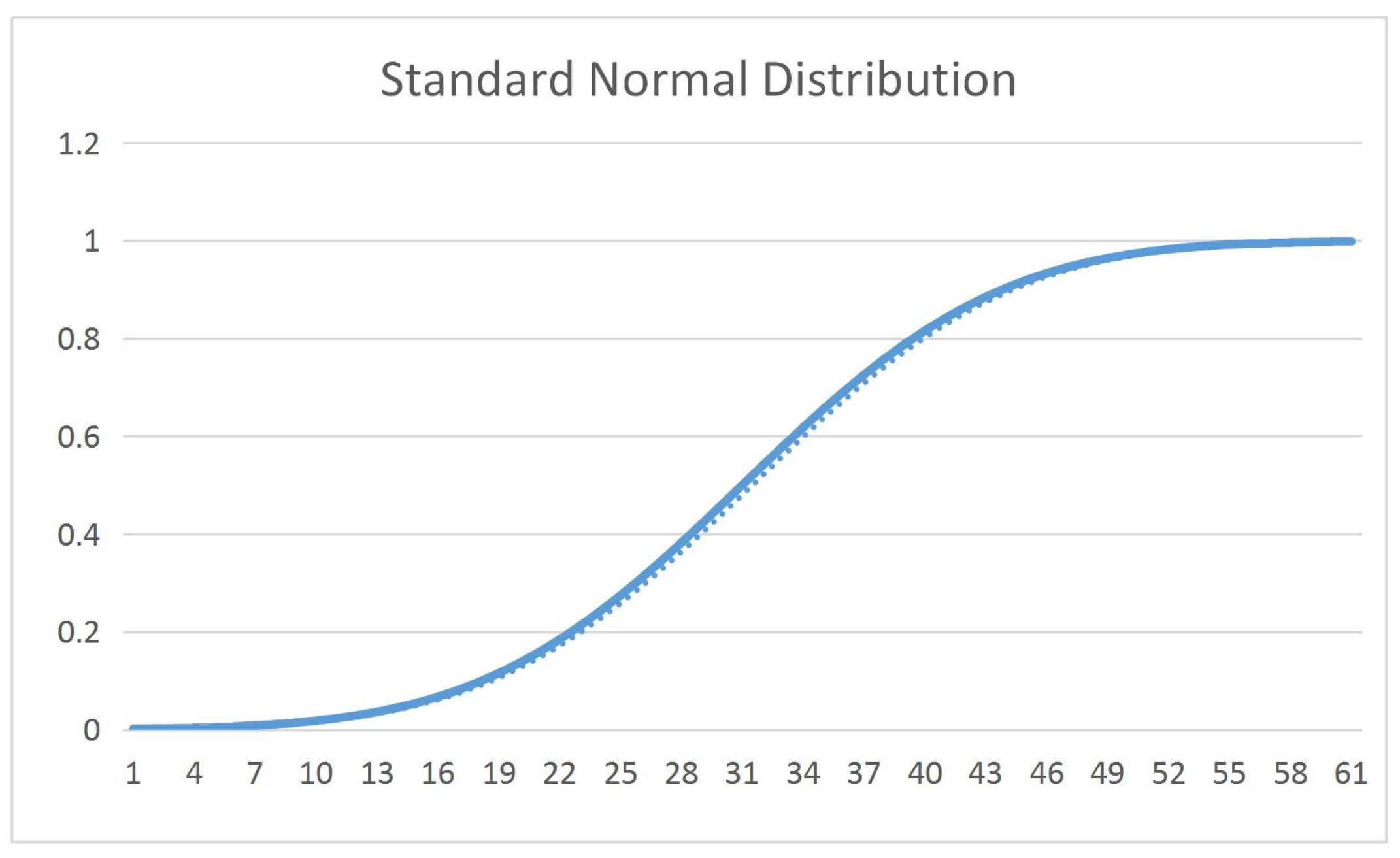
Assume an uncertain variable ξ obeys normal uncertain distribution [68]:
Consequently, obeys normal distribution, where e denotes the mean value, and σ denotes the variance (which differ from the expression in probability). Then, we call ξ obeys the normal distribution of as mean and variance, denoted by .
The figure of normal uncertainty distribution function can be seen in Figure 2.
Definition7.
The inverse uncertainty distribution of normal uncertain variable is as follows:
2.5. Correlation between Interval Distribution and Normal Uncertainty Distribution
Assume that an uncertain variable ξ obeys the normal distribution, i.e., , and the distribution function is
The inverse function is as follows:
If the function obeys the standard normal distribution, the probability of the normal uncertainty distribution variable x falling within (we call it “ ”criterion) is as follows:
This is reorganized as follows:
i.e.,
According to the “small probability event “principle, the probability of x falling outside is less than . In reality, we would consider the corresponding event happening as being almost impossible.
Since the intervals themselves originate from the results of fuzzy judgments or random sampling, we only know the upper and lower limits of the interval. It is difficult to determine the specific value, so the interval can be regarded as fuzzy numbers and can also be seen as uncertain variables. It is possible to replace the intervals with uncertain variables, taking into account the good nature of normal distribution, for an uncertain variable ξ that follows the normal distribution , according to the principle, its probability of falling within is . Therefore, we can use the constant variable ξ obeying normal distribution to approximately replace the interval :
2.5.1. Uncertain DEA Model Based on Normal Distribution
Definition8.
The equivalent uncertain normal distribution of the interval is as follows:
where
and
In the DEA model with interval input and output variables, where , , respectively, we construct an equivalent uncertain DEA Model (16) with a certain input and the largest output as follows:
is evaluated DMU in this model. The equivalent deterministic form of the Constraint (16-1) in the model is as follows:
The Model (16)’s equivalent deterministic DEA Model (17) is as follows:
is evaluated DMU in this model.
2.5.2. A Numerical Example of DEA Model Based on Normal Distribution
Assuming that there are still six DMUs of the interval model, the input indicators , and the output indicators and are interval data in Table 1, which are subjected to normal distribution. The data are shown in Table 7.
2.5.3. A Numerical Example of Equivalent Non-Linear DEA Model for Normal Distribution
Taking input and output indicators of the DMUs obeying the normal distribution of the interval data (Table 7) as the numerical example, similar to the normal distribution of the DEA Model (17), nonlinear DEA Model (18) for linear distribution is constructed as follows:
is evaluated DMU in this model.
2.5.4. A Numerical Example of Determined DEA Model for Normal Distribution
Let , for , so , i.e., have no upper and lower constraints. Similarly, , for , so , i.e., have no upper and lower constraints. The equivalent certain DEA model that obeys normal distribution is transformed into a linear Model (19) as follows:
is evaluated DMU in this model. Model (19) is solved by Lingo 11 software and the optimal solution is shown in Table 8.
As can be seen from Table 8, are non-efficient and the efficiency is lower than that of the original interval model but higher than that of the linear model. The efficiency from to presents an increasing trend.
2.5.5. Results Analysis of Three Uncertain Intervals Distribution DEA Model
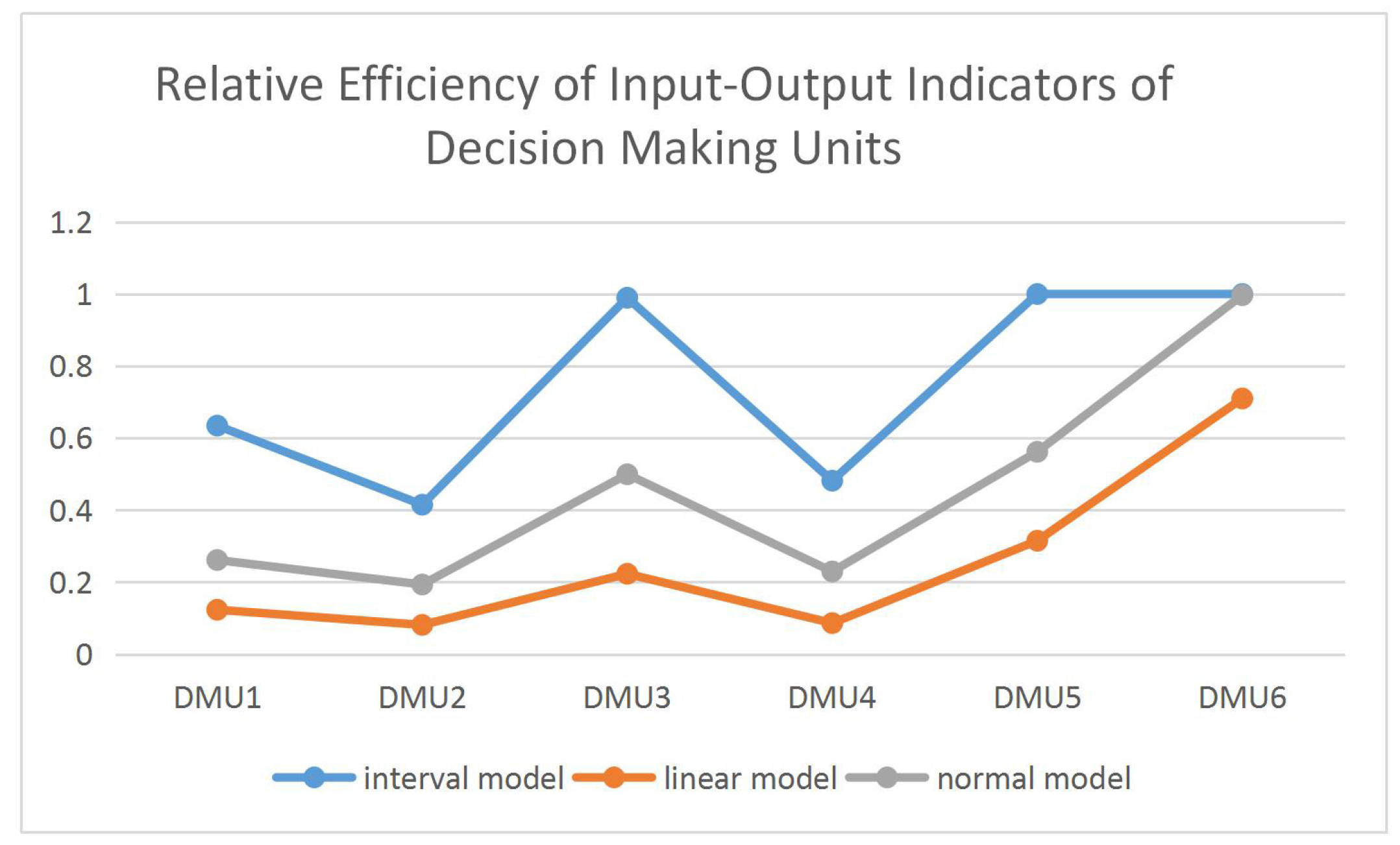
The relative efficiency figures of the original Models (7)–(9), the linear Model (15) and the normal distribution Model (19) are as follows.
The comparison analysis of the efficiency value in Figure 3 shows that efficiency sorting of DMUs is the same, but the value of the same DMU in different models is different. At the same time, the results of the normal distribution model are much better than those of the uncertain model. Therefore, we use the uncertain normal distribution model to conduct empirical analyses in the following section.
2.6. Research on the Manufacturing Output Performance of Yangtze River Delta Region Based on Environmental Pollution Constraints
For this section, we select input–output indicators of the manufacturing industry in 16 cities in the Yangtze River Delta region, China, from 2005 to 2014 to conduct relative efficiency empirical analyzes and construct uncertain DEA models based on normal distribution. We assess and rank these cities according to the relative efficiency value and conduct a corresponding analysis. Furthermore, we validate the practicability and rationality of the uncertain normal distribution DEA model.
2.6.1. Concept Definition
The geographical range of the Yangtze River Delta can be measured in narrow and generalized terms. In the narrow sense, the Yangtze River Delta encompasses 16 member cities of the Yangtze River Delta Urban Economic Coordination Committee, including the cities of Shanghai, Nanjing, Wuxi, Changzhou, Suzhou, Nantong, Yangzhou, Zhenjiang and Taizhou in Jiangsu Province and Hangzhou, Ningbo, Jiaxing, Huzhou, Shaoxing, Zhoushan and Taizhou in Zhejiang Province. In the general sense, the Yangtze River Delta refers to all regions in Shanghai, Jiangsu Province and Zhejiang Province. This study takes the narrow sense as research objectives.
Environmental quality is an intrinsic property that exists objectively in an environmental system. The deterioration of environmental quality includes ecological damage and environmental pollution. The destruction of the ecological environment is usually due to human activities, which directly or indirectly damage biological communities and non-biological elements ecosystems, and ultimately leads to the deterioration of the human living environment. Environmental pollution is the discharge of pollutants from human activities into the environment, exceeding the capacity and the self-purification capacity of the environment, so that the composition of the environment is altered, leading to the deterioration of environmental quality, affecting and undermining people’s normal production and living conditions. Pollutants mainly refer to substances that are discharged into the atmosphere, water and soil. In this paper, changes in environmental quality mainly refer to environmental pollution with less consideration of eco-environment content, so that the content of the study is targeted.
Manufacturing refers to the industry that transforms manufacturing resources (materials, energy, equipment, tools, funds, technology, information and manpower), in accordance with market demand through the manufacturing process, into large tools and useful industrial and consumer products. Manufacturing embodies a country’s productivity level, which is an important factor in distinguishing between developing and developed countries. It occupies an important share in the national economy of the developed world. The manufacturing industry referred to in this paper starts with the agro-food processing industry and ends with metal products, machinery and equipment repairing (including 31 industries: agricultural and foodstuff processing industry; food manufacturing; liquor, beverage and refined tea manufacturing; the tobacco industry; textiles; leather, fur, feather and garment industry; wood processing and footwear; bamboo, rattan, palm, straw products; furniture manufacturing; printing and recording media reproduction industry; education, engineering, sports and entertainment products manufacturing; petroleum processing, coking and nuclear fuel processing; chemical raw materials and chemical manufacturing; pharmaceutical manufacturing; rubber and plastics products industry; nonmetal mineral products industry; ferrous metals smelting and calendering processing; nonferrous metals smelting and calendering processing; metal products industry; general equipment manufacturing; special equipment manufacturing; automotive manufacturing; railways, ships, aerospace and other transport equipment manufacturing; electrical machinery and equipment manufacturing; computer, communications and other electronic equipment manufacturing; instrumentation manufacturing; other manufacturing industries; waste resources comprehensive utilization industry; metal products, machinery and equipment repair industry).
2.6.2. Indicators Selection and Data Resources
Referring to the literature [69,70,71,72,73], this paper constructs environmental indicators shown in Table 9. With regards to these indicators, water pollution is characterized by the emission of waste water and air pollution is characterized by soot and sulphur dioxide emission. The treatment of solid wastes is characterized by comprehensive utilization of waste and, lastly, energy consumption is characterized by comprehensive energy consumption.
According to the actual development situation and data feasibility of the manufacturing industry in the Yangtze River Delta, this paper studies the output–input performance of this manufacturing industry based on the constraint of environmental pollution. The 16 cities in the Yangtze River Delta include Shanghai, eight cities in Jiangsu Province, namely Nanjing, Wuxi, Changzhou, Yangzhou, Suzhou, Zhenjiang, Nantong and Xuzhou, and seven cities in Zhejiang Province, namely Hangzhou, Ningbo, Shaoxing, Jiaxing, Zhoushan, Quzhou and Taizhou.
The data in this paper are gathered from the annual statistic yearbook of each city. The waste utilization rate, waste water emission, soot emission and sulphur dioxide emission are collected with industry data calibre. The remaining indicators are collected with manufacturing calibre (Shanghai comprehensive energy consumption uses industry-calibre), minimizing the regional differences due to factors such as population and administrative area. Except for the comprehensive utilization of waste, the remaining indicators are based on the total population of each city as the denominator for processing. All monetary data is deflated in real prices based on constant price value index in 2013.
2.6.3. Indicator Elaboration
This study selects average annual number of employees (AANE), completed investment in fixed assets (CIFA), and comprehensive energy consumption (CEC) of each city, industrial waste water discharge (IWWD), industrial soot emission (ISE), industrial sulphur dioxide emission (ISD) as the input indicators and comprehensive utilization of waste(CUW), and manufacturing gross output value (GOV) as the output indicators [74,75,76,77].
2.7. Empirical Data
We process the data collected from 2005 to 2014 and the corresponding means and variances are transformed into normal distribution data, as shown in Table 10, Table 11, Table 12 and Table 13.
2.7.1. Empirical Model
We take the interval data (Table 10, Table 11, Table 12 and Table 13) of the output indicators of the DMUs that obey the normal distribution as the empirical data, which resemble the deterministic DEA Model (17) of normal distribution. The equivalent nonlinear equilibrium output Model (20) is constructed as follows:
is evaluated DMU in this model. We subsequently take the interval data (Table 10, Table 11, Table 12 and Table 13) of the input indicators of the DMU that obeyed the normal distribution as the empirical data, which resemble the deterministic DEA Model (17) with normal distribution. The equivalent nonlinear equilibrium input Model (21) is constructed as follows:
The constraints of the empirical model are as follows:
By combining Models (20)–(22), we obtain the equivalent nonlinear equilibrium DEA model of normal distribution.
Under the constraint of environmental pollution, the top four manufacturing input–output performance cities are found to be Yangzhou, Taizhou, Nantong and Shanghai, of which Yangzhou and Taizhou’s energy consumption and negative output are lower, but the per capital positive outputs are insufficient, belonging to the low-energy-consumption, low-pollution and low-output industrial structure. The energy consumption and negative output of Nantong and Shanghai are higher, but the per capital positive outputs have advantages in that they belong to the industrial structure with high energy, high pollution and high yield. However, Shanghai is at a stage of industrial transformation and the focus gradually shift from traditional to high-technology manufacturing. Nonetheless, it is still in the leading position in terms of scale and technology, so that the manufacturing output performance advantage is maintained under environmental pollution constraints.
Under the constraint of environmental pollution, Jiaxing, Quzhou and Shaoxing rank as the last three regions in manufacturing input–output performance. Their inputs and negative outputs are high, while the positive outputs are at a disadvantage, belonging to the high-input, high-pollution and low-output industrial structure.
Under the restriction of environmental pollution, although their efficiency is higher, Ningbo and Zhoushan have a slight advantage in terms of positive outputs, but the negative outputs and environmental costs of manufacturing development are higher and these regions consequently belonged to the high-pollution development model.
The Changzhou manufacturing development model is different from that of other cities. Regarding inputs, energy consumption and positive or negative outputs, Changzhou’s is significantly higher than those of other cities. Although its performance is top-ranking, the development model’s high yield is accompanied by high input, high energy consumption and high pollution. Therefore, such a model is unhealthy.
In general, except for Taizhou and Zhoushan, from the aspect of environmental pollution control of manufacturing input–output performance, cities in Zhejiang Province rank lower than other cities; there is a gap in the development level of the manufacturing industry between Shanghai and Jiangsu Province.
As for the Yangtze River coast, except for Shanghai, Yangzhou and Nantong, the manufacturing output performance under the constraint of environmental pollution of regions in the south is lower than that of regions in the north. Although the manufacturing levels in the south are high, the environmental costs are also higher.
3. Conclusions
In practice, input and output variables are usually interval data in the complex efficiency evaluation. The traditional approach is to consider the upper and lower limits of the interval data and many researchers consequently constructed models with upper and lower limits for evaluation, which inevitably leads to the lack of some important information. This study attempted to overcome these defects by studying the problems of input–output efficiency evaluation with interval data through two research angles.
The first perspective did not consider the distribution of interval data. Introducing the tuning parameters, α, the interval data were transformed into determination data. By using optimization methods, the input–output performance evaluation value was acquired. The advantage of this method was that the overall interval information could be considered more comprehensive and was conducive to the improvement of the non-efficient decision units.
The second perspective did consider the distribution characteristics of interval data. Based on the uncertainty theory proposed by Liu [68], the DEA evaluation model with interval data was constructed from dimensions of linear uniform distribution and normal distribution with uncertainty:
i
Linear uniform distribution model: According to the uncertain optimization theory, the DEA uncertainty evaluation model for linear uniform distribution was transformed into a deterministic nonlinear DEA evaluation model, which was further transformed into a deterministic linear DEA evaluation model.
ii
Uncertainty model of normal distribution: Based on uncertain optimization theory, we adopted the ‘’ rule. First, we transformed the input–output interval indicators into an approximate normal distribution of the input–output DEA evaluation efficiency uncertainty optimization model. Then, we transformed it into an equivalent normal distribution of input–output DEA deterministic evaluation model.
iii
The advantage of these two kinds of transformation is that it can further reduce the computational cost of the model optimization solution and obtain the optimal solution of the uncertain model.
iv
The results of empirical analysis showed that the optimal solution of the normal distribution model was better than that of the linear distribution. Therefore, based on the normal distribution DEA evaluation model, this paper studied the input–output performance evaluation of the manufacturing industry in the Yangtze River Delta under the constraint of environmental pollution.
The paper focused on the regions of 16 member cities of Yangtze River Delta Regional Urban Economic Coordination Committee. We collected the manufacturing data of these cities from 2005 to 2014. According to the means and variances of these data, they were transformed into approximate normal distribution data indicators. Using the previously constructed normal distribution input–output DEA evaluation efficiency deterministic optimization model, we analyzed each city’s sorted input–output performance results. We consequently offered corresponding countermeasures and suggestions according to the differences in industrial structure in different cities.
The authors would like to thank the editor and all anonymous referees for their valuable comments and suggestions. This research was supported by the National Natural Science Foundation of China , the Six Talent Peaks Project in Jiangsu Province (2014-JY-014), and the Natural Science Foundation of Jiangsu , ’333 Project’ research projects funded project (BRA2017456).
Author Contributions
Xiaoqing Chen was responsible for the model development and first draft, and finalized the manuscript. Zaiwu Gong conceived the main idea of the experiments and supervised the whole process of model development and manuscript drafting. All coauthors made significant contributions to the research contained in this article.
Conflicts of Interest
The authors declare no conflict of interest.
Abbreviations
The following abbreviations are used in this manuscript:
DEA
Data Envelopment Analysis
DMU
decision-making units
YRD
Yangtze River Delta
TP
Total Population
CUW
comprehensive utilization of waste
AANE
average annual number of employees
CIFA
completed investment in fixed assets
CEC
comprehensive energy consumption
IWWD
industrial waste water discharge
ISE
industrial soot emission
ISD
industrial sulphur dioxide emission
GOV
manufacturing gross output value
References
Fujii, H.; Managi, S. Wastewater management efficiency and determinant factors in the Chinese industrial sector from 2004 to 2014. Water2017, 9, 586. [Google Scholar] [CrossRef]
Fujii, H.; Cao, J.; Managi, S. Decomposition of Productivity Considering Multi-environmental Pollutants in Chinese Industrial Sector. Rev. Dev. Econ.2015, 19, 75–84. [Google Scholar] [CrossRef]
Fujii, H.; Cao, J.; Managi, S. Firm-level environmentally sensitive productivity and innovation in China. Appl. Energy2016, 184, 915–925. [Google Scholar] [CrossRef]
Yang, Q.; Kaneko, S.; Fujii, H.; Yoshida, Y. Do exogenous shocks better leverage the benefits of technological change in the staged elimination of differential environmental regulations? Evidence from China’s cement industry before and after the 2008 Great Sichuan Earthquake. J. Clean. Prod.2017, 164, 1167–1179. [Google Scholar] [CrossRef]
Charnes, A.; Cooper, W.W.; Rhodes, E. Measuring the efficiency of decision making units. Eur. J. Oper. Res.1978, 2, 429–444. [Google Scholar] [CrossRef]
Lu, K.; Nie, C.L. Application of Data Envelopment Analysis in Analysis of Maintenance Support Efficiency. Mod. Def. Technol.2017, 1, 167–172. [Google Scholar]
Li, J.J. Research on innovation performance of Listed Companies in Anhui Province—Based on DEA analysis. J. Chifeng Univ.2016, 24, 78–80. [Google Scholar]
Huang, H.S.; Yang, H.G. An analysis of the effectiveness of investment in Chengdu based on DEA model. China Mark. China Mark.2016, 47, 22–25. [Google Scholar]
Tan, J.; Luo, Z.Y.; Xu, G.W. Evaluation on Input Performance of Technological Innovation Based on CCR, BCC and SE-DEA Models. Sci. Technol. Econ.2017, 1, 36–40. [Google Scholar]
Kwon, D.S.; Cho, J.H.; Sohn, S.Y. Comparison of technology efficiency for CO2 emissions reduction among European countries based on DEA with decomposed factors. J. Clean. Prod.2017, 151, 109–120. [Google Scholar] [CrossRef]
Toloo, M. On finding the most BCC-efficient DMU: A new integrated MIP-DEA model. Appl. Math. Model.2012, 36, 5515–5520. [Google Scholar] [CrossRef]
Guo, I.L.; Lee, H.S.; Lee, D. An integrated model for slack-based measure of super-efficiency in additive DEA. Omega2017, 67, 160–167. [Google Scholar] [CrossRef]
Gutierrez, E.; Aguilera, E.; Lozano, S.; Guzmán, G.I. A two-stage DEA approach for quantifying and analyzing the inefficiency of conventional and organic rain-fed cereals in Spain. J. Clean. Prod.2017, 149, 335–348. [Google Scholar] [CrossRef]
Li, L.B.; Liu, B.L.; Liu, W.L.; Chiu, Y.H. Efficiency evaluation of the regional high-tech industry in China: A new framework based on meta-frontier dynamic DEA analysis. Socio-Econ. Plan. Sci.2017. [Google Scholar] [CrossRef]
Aryana, B. New version of DEA compressor for a novel hybrid gas turbine cycle: TurboDEA. Energy2016, 111, 676–690. [Google Scholar] [CrossRef]
Zhu, J.X.; Sun, Y.H.; Yang, L.M. Research on Stochastic DEA Model for Undesirable Outputs Evaluation. J. Qual. Econ.2015, 3, 73–77. [Google Scholar]
Shwartz, M.; Burgess, J.F.; Zhu, J. A DEA based composite measure of quality and its associated data uncertainty interval for health care provider profiling and pay-for-performance. Eur. J. Oper. Res.2016, 253, 489–502. [Google Scholar] [CrossRef]
Chi, G.T.; Du, Y.Q.; He, X.G.; Liu, J.B. Research on Loan Pricing Model Based on the Interval DEA. Oper. Res. Manag. Sci.2015, 5, 189–196. [Google Scholar]
Fan, J.P.; Yue, W.Z.; Wu, M.Q. Dealing with interval DEA based on error propagation and entropy. Syst. Nato Pract.2016, 5, 1293–1303. [Google Scholar]
Chen, X.Q.; Gong, Z.W. DEA Efficiency of Energy Consumption in China’s Manufacturing Sectors with Environmental Regulation Policy Constraints. Sustainability2017, 9, 210. [Google Scholar] [CrossRef]
Olfat, L.; Amiri, M.; Soufi, J.B.; Pishdar, M. A dynamic network efficiency measurement of airports performance considering sustainable development concept: A fuzzy dynamic network-DEA approach. J. Air Transp. Manag.2016, 57, 272–290. [Google Scholar] [CrossRef]
Aggelopoulos, E.; Georgopoulos, A. Bank branch efficiency under environmental change: A bootstrap DEA on monthly Profit and Loss accounting statements of Greek retail branches. Eur. J. Oper. Res.2017, 261, 1170–1188. [Google Scholar] [CrossRef]
Vlontzos, G.; Pardalos, P.M. Assess and prognosticate green house gas emissions from agricultural production of EU countries, by implementing, DEA Window analysis and artificial neural networks. Renew. Sustain. Energy Rev.2017, 76, 155–162. [Google Scholar] [CrossRef]
Cooper, W.W.; Huang, Z.; Lelas, V.; Li, S.X.; Olesen, O.B. Chance constrained programming formulations for stochastic characterizations of efficiency and dominance in DEA. J. Prod. Anal.1998, 9, 53–79. [Google Scholar] [CrossRef]
Ding, Q.Y.; Wang, L. Empirical study on scale economy of securities companies: Based on methods of DEA and translog cost function. J. Shenyang Univ. Technol.2014, 6, 529–534. [Google Scholar]
Zhang, Z.H. Influencing Factors and Performance Analysis of Land Transfer in Shanxi; Northwest University: Xian, China, 2012. [Google Scholar]
Duan, Z.P. Analysis on Energy Utilization-Efficiency of the Main Industries in Jiangxi Province; Nanchang University: Nanchang, China, 2010. [Google Scholar]
Alzamora, R.M.; Apiolaza, L.A. A DEA approach to assess the efficiency of radiata pine logs to produce New Zealand structural grades. J. For. Econ.2013, 19, 221–233. [Google Scholar] [CrossRef]
Lin, B.; Xie, C. Energy substitution effect on transport industry of China-based on trans-log production function. Energy2014, 67, 213–222. [Google Scholar] [CrossRef]
Bounneche, M.D.; Boubchir, L.; Bouridane, A.; Nekhoul, B.; Ali-Chérif, A. Multi-spectral palmprint recognition based on oriented multiscale log-Gabor filters. Neurocomputing2016, 205, 274–286. [Google Scholar] [CrossRef]
Zhang, H.X. Study on chance constrained stochastic DEA model based on exponential distribution. Univ. Electron. Sci. Technol. China2016, 8, 356–369. [Google Scholar]
Peng, Y.; Chen, S.Y.; Sheng, W.W.; Pu, Y. Efficiency Based on the Two-stage Correlative DEA Malmquist Index on Western Regional Technical Innovation. Oper. Res. Manag. Sci.2013, 3, 162–168. [Google Scholar]
Li, G.C.; Fan, L.X.; Cheng, G.; Feng, Z.C. Total factor productivity growth in agriculture: A new window based DEA productivity index. J. Agrotechnol.2013, 5, 4–17. [Google Scholar]
Wang, W.G.; Ma, Y.Y. The Efficiency of Regional Logistics Industry in China-Based on the Three-stage DEA Model Using Malmquist-luenberger Index. Syst. Eng.2012, 3, 66–75. [Google Scholar]
Dai, X.; Kuosmanen, T. Best-practice benchmarking using clustering methods: Application to energy regulation. Omega2014, 42, 179–188. [Google Scholar] [CrossRef]
Jeang, A. Robust DEA methodology via computer model for conceptual design under uncertainty. J. Intell. Manuf.2017. [Google Scholar] [CrossRef]
Yuan, J.; Wu, Z.W. Research on Transfer Efficiency of High-Speed Rail Station Based on DEA Model. Luoyang Inst. Sci. Technol.2017, 1, 48–51. [Google Scholar]
Li, S.H.; Xiong, C. Analysis on the Efficiency and Public Satisfaction of Local Government Fiscal Expenditure on Social Security. Chin. Public Admin.2016, 2, 104–111. [Google Scholar]
Hu, X.W.; Wei, Y.B. Evaluation of Urban Public Transport Service Satisfaction Degree in Cold Regions’ Winter Based on DEA Method. J. Beijing Univ. Technol.2015, 10, 1566–1573. [Google Scholar]
Dai, Q.Z.; Lei, X.Y.; Li, Y.J.; Xie, Q.W. Allocating emissions based on DEA and maximizing the whole satisfaction degree. Syst. Nato Pract.2014, 4, 917–924. [Google Scholar]
Shabanpour, H.; Yousefi, S.; Saen, R.F. Future planning for benchmarking and ranking sustainable suppliers using goal programming and robust double frontiers DEA. Transp. Res. Part D Transp. Environ.2017, 50, 129–143. [Google Scholar] [CrossRef]
Nazari-Shirkouhi, S.; Keramati, A. Modeling customer satisfaction with new product design using a flexible fuzzy regression-DEA algorithm. Appl. Math. Model.2017, 10, 1566–1573. [Google Scholar]
Xi, W.; Li, A. The measurement of industrial capital service and the difference of production efficiency. Price Theory Pract.2016, 12, 155–158. [Google Scholar]
Liang, S.; Zeng, X.T.; Li, Y.P.; Qiao, X.L. The Effect Evaluation of Operation and Management on Soil and Water Conservation Project Based on Entropy Fuzzy Credibility-constrained DEA Method. China Rural Water Hydropower2015, 8, 94–97. [Google Scholar]
Wang, M.Q.; Li, Y.J. Non-radial Fuzzy DEA Model Based on Credibility Measure. Fuzzy Syst. Math.2010, 6, 110–116. [Google Scholar]
Fasanghari, M.; Amalnick, M.S.; Anvari, R.T.; Razmi, J. A novel credibility-based group decision making method for Enterprise Architecture scenario analysis using Data Envelopment Analysis. Appl. Soft Comput.2015, 32, 347–368. [Google Scholar] [CrossRef]
Azadeh, A.; Kokabi, R. Z-number DEA: A new possibilistic DEA in the context of Z-numbers. Adv. Eng. Inform.2016, 30, 604–617. [Google Scholar] [CrossRef]
Salvador-Carulla, L.; Torres-Jiménez, M.; GarcÍa-Alonso, C.R.; Fernández-Rodríguez, V. Evaluation of system efficiency using the Monte Carlo DEA: The case of small health areas. Eur. J. Oper. Res.2015, 242, 525–535. [Google Scholar]
Perelman, S.; SantÍn, D. How to generate regularly behaved production data? A Monte Carlo experimentation on DEA scale efficiency measurement. Eur. J. Oper. Res.2009, 199, 303–310. [Google Scholar] [CrossRef]
Cordero, J.M.; Santín, D.; Sicilia, G. Testing the accuracy of DEA estimates under endogeneity through a Monte Carlo simulation. Eur. J. Oper. Res.2015, 244, 511–518. [Google Scholar] [CrossRef]
Oh, S.C.; Shin, J. The impact of mismeasurement in performance benchmarking: A Monte Carlo comparison of SFA and DEA with different multi-period budgeting strategies. Eur. J. Oper. Res.2015, 240, 518–527. [Google Scholar] [CrossRef]
Andor, M.; Hesse, F. The StoNED age: The departure into a new era of efficiency analysis ? A monte carlo comparison of StoNED and the ”oldies”(SFA and DEA). J. Prod. Anal.2014, 41, 85–109. [Google Scholar] [CrossRef]
Azadeh, A.; Ahvazi, M.P.; Haghighii, S.M.; Keramati, A. Simulation optimization of an emergency department by modeling human errors. Simul. Model. Pract. Theory2015, 67, 117–136. [Google Scholar] [CrossRef]
Wu, Q. An Applied Study of Financial Distress Warning of Listed Companies Base on Logostic Model and Bayesian Network; Jilin University: Changchun, China, 2011. [Google Scholar]
Jia, J.X. Dynamic selection method of manufacturers to customers—Application of DEA method and Bayesian correction method. Mod. Manag. Sci.2006, 4, 39–40. [Google Scholar]
Tsionas, E.G.; Papadakis, E.N. A Bayesian approach to statistical inference in stochastic DEA. Omega2010, 38, 309–314. [Google Scholar] [CrossRef]
Chiang, T.A.; Che, Z.H. A fuzzy robust evaluation model for selecting and ranking NPD projects using Bayesian belief network and weight-restricted DEA. Expert Syst. Appl.2010, 37, 7408–7418. [Google Scholar] [CrossRef]
Tsionas, E.G.; Papadakis, E.N. Combining DEA and stochastic frontier models: An empirical Bayes approach. Eur. J. Oper. Res.2003, 147, 499–510. [Google Scholar] [CrossRef]
Mitropoulos, P.; Talias, M.A.; Mitropoulos, I. Combining stochastic DEA with Bayesian analysis to obtain statistical properties of the efficiency scores: An application to Greek public hospitals. Eur. J. Oper. Res.2015, 243, 302–311. [Google Scholar] [CrossRef]
Khodabakhshi, M.; Asgharian, M. An input relaxation measure of efficiency in stochastic data envelopment analysis. Appl. Math. Model.2009, 33, 2010–2023. [Google Scholar] [CrossRef]
Eslami, R.; Khodabakhshi, M.; Jahanshahloo, G.R.; Lotfi, F.H.; Khoveyni, M. Estimating most productive scale size with imprecise-chance constrained input-output orientation model in data envelopment analysis. Comput. Ind. Eng.2012, 63, 254–261. [Google Scholar] [CrossRef]
Zhou, X.; Pedrycz, W.; Kuang, Y.; Zhang, Z. Type-2 fuzzy multi-objective DEA model: An application to sustainable supplier evaluation. Appl. Soft Comput.2016, 46, 424–440. [Google Scholar] [CrossRef]
Yu, X.W.; Lei, M.; Wang, Q.W.; Deng, J. Chinese Commercial Bank’s Efficiency (2005–2011): Based on Time-Series Regression and Chance-constrained DEA model. China J. Manag. Sci.2012, S1, 356–362. [Google Scholar]
Fujii, H.; Managi, S. An evaluation of inclusive capital stock for urban planning. Ecosyst. Health Sustain.2015, 2. [Google Scholar] [CrossRef]
Zarepisheh, M.; Soleimani-Damaneh, M. A dual simplex-based method for determination of the right and left returns to scale in DEA. Eur. J. Oper. Res.2009, 194, 585–591. [Google Scholar] [CrossRef]
Yagi, M.; Fujii, H.; Hoang, V.; Managi, S. Environmental efficiency of energy, materials, and emissions. J. Environ. Manag.2015, 161, 206–218. [Google Scholar] [CrossRef] [PubMed]
Liu, B. Uncertainty theory. In Uncertainty Theory; Springer: Berlin/Heidelberg, Germany, 2007; pp. 205–234. [Google Scholar]
Zhao, H.X.; Jiang, X.W.; Cui, J.X. Shifting Path of Industrial Pollution Gravity Centers and Its Driving Mechanism in Pan-Yangtze River Delta. Environ. Sci.2014, 11, 504–512. [Google Scholar]
Song, J.; Wang, H.X.; Liu, S.Y. Quantitative assessment of stress of economic development to environment using ecological stress index. China J. WIT2014, 22, 368–374. [Google Scholar] [CrossRef]
Wang, Q.; Liu, Y.L.; Wu, Y.Y.; Wen, Y.L. Analysis of Spatial Characteristics of Emission Intensity of the Main Pollutants in China. Int. Environ. Sci.2015, 3, 57–61. [Google Scholar]
Chen, Z.H.; Lei, Z.J. The spatial-temporal characteristics and economic drivers of environmental pollution changes in China. Geogr. Res.2015, 11, 2165–2178. [Google Scholar]
Cao, Z.L.; Yang, J. Manufacturing Level Estimation and Trend Analysis of Environmental Pollution in China. Econ. Geol.2013, 4, 107–113. [Google Scholar]
Wang, L.; Gong, Z.; Gao, G.; Wang, C. Can energy policies affect the cycle of carbon emissions? Case study on the energy consumption of industrial terminals in Shanghai, Jiangsu and Zhejiang. Ecol. Indic.2017, 83, 1–12. [Google Scholar] [CrossRef]
Fujii, H.; Managi, S. Optimal production resource reallocation for CO2 emissions reduction in manufacturing sectors. Glob. Environ. Chang.2015, 35, 505–513. [Google Scholar] [CrossRef]
Lee, B.L.; Wilson, C.; Pasurka, C.A.; Fujii, H.; Managi, S. Sources of airline productivity from carbon emissions: An analysis of operational performance under good and bad outputs. J. Prod. Anal.2017, 47, 223–246. [Google Scholar] [CrossRef]
Kumar, S.; Fujii, H.; Managi, S. Substitute or complement? Assessing renewable and nonrenewable energy in OECD countries. Appl. Econ.2015, 47, 1438–1459. [Google Scholar] [CrossRef]
Figure 1.
Linear uncertainty distribution.
Figure 1.
Linear uncertainty distribution.
Figure 2.
Normal uncertainty distribution.
Figure 2.
Normal uncertainty distribution.
Figure 3.
DEA efficiency comparisons of three kind of uncertainty distribution.
Figure 3.
DEA efficiency comparisons of three kind of uncertainty distribution.
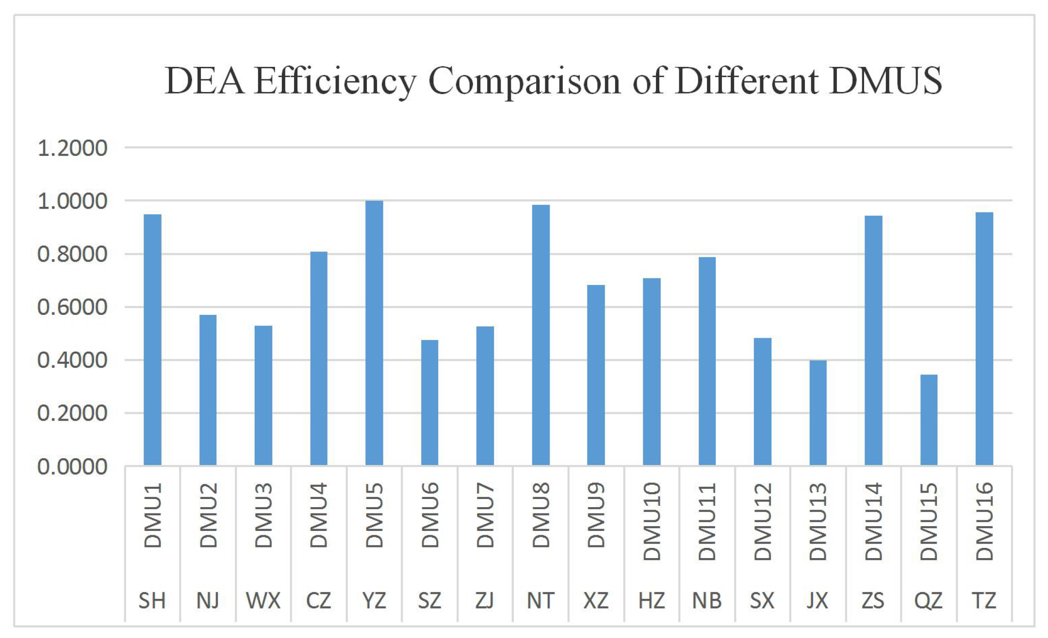
Figure 4.
DEA efficiency comparison of different DMUs.
Figure 4.
DEA efficiency comparison of different DMUs.
Gong, Z.; Chen, X.
Analysis of Interval Data Envelopment Efficiency Model Considering Different Distribution Characteristics—Based on Environmental Performance Evaluation of the Manufacturing Industry. Sustainability2017, 9, 2080.
https://doi.org/10.3390/su9122080
AMA Style
Gong Z, Chen X.
Analysis of Interval Data Envelopment Efficiency Model Considering Different Distribution Characteristics—Based on Environmental Performance Evaluation of the Manufacturing Industry. Sustainability. 2017; 9(12):2080.
https://doi.org/10.3390/su9122080
Chicago/Turabian Style
Gong, Zaiwu, and Xiaoqing Chen.
2017. "Analysis of Interval Data Envelopment Efficiency Model Considering Different Distribution Characteristics—Based on Environmental Performance Evaluation of the Manufacturing Industry" Sustainability 9, no. 12: 2080.
https://doi.org/10.3390/su9122080
Note that from the first issue of 2016, this journal uses article numbers instead of page numbers. See further details here.
Article Metrics
No
No
Article Access Statistics
For more information on the journal statistics, click here.
Multiple requests from the same IP address are counted as one view.
Gong, Z.; Chen, X.
Analysis of Interval Data Envelopment Efficiency Model Considering Different Distribution Characteristics—Based on Environmental Performance Evaluation of the Manufacturing Industry. Sustainability2017, 9, 2080.
https://doi.org/10.3390/su9122080
AMA Style
Gong Z, Chen X.
Analysis of Interval Data Envelopment Efficiency Model Considering Different Distribution Characteristics—Based on Environmental Performance Evaluation of the Manufacturing Industry. Sustainability. 2017; 9(12):2080.
https://doi.org/10.3390/su9122080
Chicago/Turabian Style
Gong, Zaiwu, and Xiaoqing Chen.
2017. "Analysis of Interval Data Envelopment Efficiency Model Considering Different Distribution Characteristics—Based on Environmental Performance Evaluation of the Manufacturing Industry" Sustainability 9, no. 12: 2080.
https://doi.org/10.3390/su9122080
Note that from the first issue of 2016, this journal uses article numbers instead of page numbers. See further details here.


