Spatial Patterns and the Regional Differences of Rural Settlements in Jilin Province, China

1
College of Earth Sciences, Jilin University, Changchun 130012, China
2
Key Laboratory of Wetland Ecology and Environment, Northeast Institute of Geography and Agroecology, Chinese Academy of Sciences, Changchun 130102, China
3
Institute of Geographic Sciences and Natural Resources Research, Chinese Academy of Sciences, Beijing 100049, China
4
College of Resources and Environment, University of Chinese Academy of Sciences, Beijing 100049, China
*
Author to whom correspondence should be addressed.
Sustainability 2017, 9(12), 2170; https://doi.org/10.3390/su9122170
Submission received: 24 September 2017
/
Revised: 21 November 2017
/
Accepted: 21 November 2017
/
Published: 25 November 2017
(This article belongs to the Special Issue Sustainable Land Uses and Rural Governance)
Abstract
:The spatial patterns of rural settlements are important for understanding the drivers of land use change and the relationship between human activity and environmental processes. It has been suggested that the clustering of houses decreases the negative effects on the environment and promotes the development of the countryside, but few empirical studies have quantified the spatial distribution patterns of houses. Our aim was to explore the regional differences in rural settlement patterns and expand our understanding of their geographic associations, and thus contribute to land use planning and the implementation of the policy of “building a new countryside”. We used spatial statistical methods and indices of landscape metrics to investigate different settlement patterns in three typical counties within different environments in Jilin Province, Northeast China. The results indicated that rural settlements in these three counties were all clustered, but to a varied degree. Settlement density maps and landscape metrics displayed uniformity of the settlement distributions within plain, hill, and mountainous areas. Influenced by the physical environment, the scale, form, and degree of aggregation varied. Accordingly, three types of rural settlements were summarized: a low-density, large-scale and sparse type; a mass-like and point-scattered type; and a low-density and high cluster-like type. The spatial patterns of rural settlements are the result of anthropogenic and complex physical processes, and provide an important insight for the layout and management of the countryside.
1. Introduction
Rural development has been highlighted in the form of policy with the industrialization and urbanization of a country reaching a certain stage. For example, the “Rural White Papers” of England, Scotland, and Wales were comprehensive reports of the governments’ policies on issues relating to rural areas [1]. In the 1970s, the “New Countryside Campaign” was carried out by South Korea to accelerate the development of rural areas [2]. For China, since the opening up policy of 1978, and the economic development and urbanization that followed, a series of rural problems have come out, including: the shrinking of cultivated land, the inefficient and extensive utilization of resources, small-scale and disorderly distributions of rural settlements, the hollow village problem, etc. [3]. All of these widened the income gap between rural and urban residents, and led to a weak foundation of the agricultural sector for speeding up regional development [1]. Under the circumstances, the “building a new countryside” strategy was laid out by the central government of China, which expected to solve all of the above problems through coordinating the development of urban and rural areas. Taking the village as a place where local communities live and work, the specific solutions to this policy were realized through centralizing rural settlements, improving infrastructure, and directing developments according to local environmental conditions. Therefore, to realize the sustainable management of rural areas, a reasonable rural planning is necessary and thus can reduce the impact on the environment [4].
Rural settlements are places to inhabit, produce, and live for rural people, and are interactive results of the surrounding natural, economic, social, and cultural environment [5]. Residential settlements and ancillary infrastructure development have been recognized as primary causes of anthropogenic landscape changes in many countries [6]. The patterns of spatial dispersion and expansion in China and other countries have received enough attention at the urban fringe. However, all of these concentrated on “suburban sprawl” [6,7,8], or the importance of the urban–rural gradient that runs from the densely urbanized inner city to exurban environments [9,10,11,12,13], but neglected the profound impact brought by the settlements located in more remote rural areas.
Many recent case studies have been conducted to analyze the area, shape, and density, as well as the evolution, of the landscape of rural settlements [2,14,15]. In China, due to the implementation of the policy to build a socialist countryside in recent years, more attention has been paid to the problems regarding rural urbanization, rural communities, the “hollowing out” of rural settlements, and the optimized regulation of rural settlements [16,17,18,19]. However, analysis of the spatial distribution and pattern of rural settlements is of great importance for understanding the influence of landscape changes and adopting policies to guide rural development. Therefore, the characteristics of typical patterns and the spatial reconstruction of rural settlements have become a hot issue in academic circles [20,21].
Several approaches have been developed to reveal the spatial characteristics of rural settlements with regular data [22,23,24]. In the past 20 years, due to the application of geographic information system (GIS), the spatial pattern of residential land has undergone a revolutionary change. Since Hodder and Orton suggested rather complicated and cumbersome models in the early 1970s, sophisticated built-in tests have been available in the ArcGIS software packages (Fletcher, 2008). However, the application of these tools is still in the initial stages [25,26].
Northeast China is a famous grain-producing region in China. The grain production capacity accounted for 19.3% of the country’s total in 2015 [27], and maize production accounted for approximately 30% of the nation’s total production [28]. The rural problem of northeast China has always been a matter of national concern, and rural development of northeast China has become a prerequisite for regional development. Jilin Province is a major agricultural province in northeast China, and arable land accounts for more than 30% of the total area. In addition, there are significant regional differences in the natural environment, economic development, and cultural context from west to east. Accordingly, the development patterns of different counties in Jilin Province should be discrepantly influenced by their particular geographical factors [18,29]. Understanding this spatial pattern and its geographical linking could provide valuable insights for planners and decision-makers to plan and renovate the rural settlements in different regions [19].
Our objectives are to: (1) compare spatial distribution patterns of rural settlements in different regions; (2) interpret the geographical factors affected by the spatial patterns of settlements; and (3) explore the development of modes suited to regional characteristics.
2. Materials and Methods
2.1. Study Area
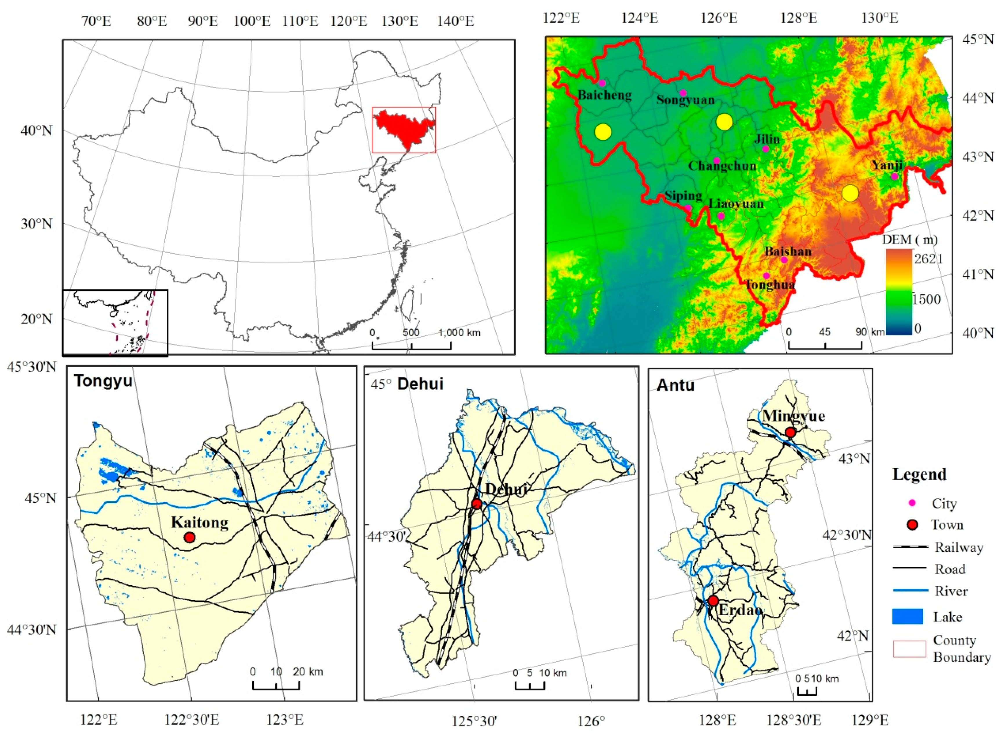
Jilin Province is located in northeast China (40°52′N to 46°18′N, 121°38′E to 131°19′E) (Figure 1). The total land area is approximately 187,400 km2. The altitude drops gently from the southeast to the northwest, with the vast Songnen Plain in the mid-west of the province. The prevalent climate in the study area is a continental monsoon, and the annual average precipitation changes between 350 mm and 1500 mm gradually from east to west. Jilin Province is the largest commercial grain-producing base of China. A study on its rural settlements is useful for regional land management and economic development. In this paper, three typical counties, Tongyu, Dehui, and Antu, were selected from different regions as study areas.
Located in western Jilin Province, Tongyu extends from 44°13′57″N to 45°16′N in latitude and from 122°02′13″E to 123°30′57″E in longitude, with a territory of 8459 km2. The climate is characterized by a temperate continental monsoon with four distinct seasons. The average annual temperature is 5.1 °C, and extreme temperatures range from−32 °C to 38.9 °C. The mean annual precipitation amounts to 400–500 mm, 70–80% of which is concentrated in the summer season. Accordingly, mean annual evaporation is up to 1500–1900 mm. Its landform is generally similar to a dustpan, because its eastern, southern, and western parts are comparatively higher than its northern part.
Dehui is situated in the middle of Jilin province (125°45′E to 126°23′E, 43°32′N to 44°45′N), covering an area of approximately 3435 km2. The elevation ranges from 149 m to 241 m, dropping slightly from the south to the north and fluctuating from east to west across the study area. The Songhua River, Yitong River, Yingma River, and Wukai River run through the middle of Dehui. It has a semi-humid, continental, monsoon-type climate with an annual mean temperature of 4.4 °C, and an annual average precipitation of 530 mm. Dehui is one of the best agricultural demonstration regions in Jilin Province, with farmland accounting for 70% of the total land [29].
Antu is located in the east of Jilin Province and covers an area of 7438 km2. The topography fluctuates across the study area, with a relative elevation of 2357 m, and drops from southeast to northwest, showing the characteristics of a narrow strip. There are convenient traffic conditions here, and the Minglong highway runs from north to south. Antu is rich in forests, water, and mineral resources, and the tourism industry developed quickly based on the scenic Changbai Mountains.
2.2. Interpretation of Rural Settlements
To establish the land use data sets, a total of six scenes of Landsat OLI images (30 m spatial resolution) were used for the land use classification in 2015. All of the images used in the classification were false colors composed of four, three, and two bands using the RGB method, and georeferenced to 1:100,000 relief maps using at least 20 ground control points (GCPs) for each scene. The root mean squared error (RMS error) of the geometric reference was controlled within 1.5 pixels.
Land use classified data of the study area were obtained by the object-oriented classification (using eCognition 8.64 software [30]) combined with the nearest neighbor classifiers and visual interpretations (Figure 2). First, multi-resolution segmentation was used to process the Landsat OLI imageries, and then, the images were grouped into homogeneous pixels representing individual objects [31]. In this process, the scale, shape, and compactness were selected as image segmentation parameters. We classified image objects into different classes using the nearest neighbor classifiers and visual interpretation after segmentation. In our study, there were eight aggregated classes of land use types: rural settlement, urban built-upland, cropland, forestland, grassland, wetland, water body, and barren land. The overall accuracy of the land use maps interpreted from remote sensing images exceeded 90% (91.3% for Tongyu, 91.5% for Dehui, and 90.9% for Antu, respectively). The results indicated that 99% of the polygon boundaries showed a shift of less than 1.5 pixels (45 m) from the real boundary.
2.3. Spatial Statistic Method
Using data of rural settlements interpreted from Landsat imagery, the central points of rural settlements were extracted. We used spatial statistic methods, such as Ripley’s K, kernel density estimation (KDE), and Getis–Ord General G methods to interpret the spatial distribution, spatial variation, spatial agglomeration, and other heterogeneous characteristics of the rural settlements in the study area. These calculations were realized using the GIS software ArcGIS 10.3.
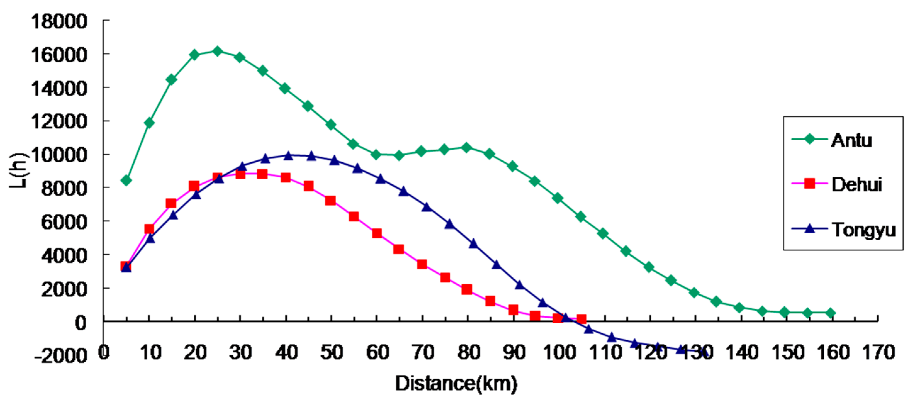
Ripley’s K function is a tool used to characterize the strength of spatial dependence at multiple scales in a spatial pattern. The K function has been widely used to identify clustering, randomness, or regularity among events in a spatial point pattern [32]. The formula is as follows:
where A is the area of the study region, n is the number of settlements, d represents the spatial scale, δij(d) is a weight, dij refers to the distance between settlement i and settlement j, and δij = 1 (dij ≤ d) or δij = 0 (dij > d). In order to achieve the linearly-expected value and stability of the standard deviance, Besag replaced K(d) with L(d), whose expected value is zero under the assumption of a totally random spatial distribution [33]. The graph of L(d) can be used to describe the spatial pattern of a multi-scale landscape. When L(d) > 0, rural settlements show a clustered distribution; when L(d) < 0, a spatial model of uniform distribution is demonstrated; and when L(d) = 0, a completely random distribution is shown.
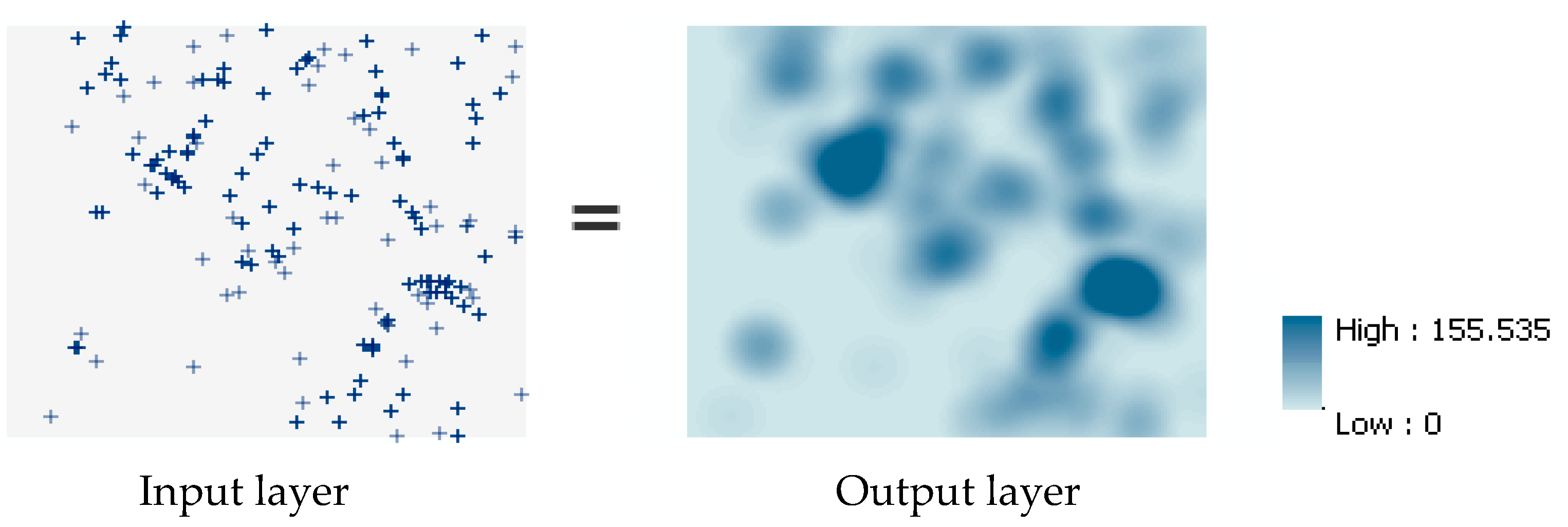
The KDE calculates the density of features in a fixed neighborhood around those features (Figure 3). The distance from the point to the reference position is calculated using the mathematical function to obtain the sum of all of the surfaces in the reference position and the peaks and kernel of these points are established to produce a smooth and continuous surface.
KDE is described as following:
where f(x,y) is the estimated density at position (x,y), n is the number of observation points, h represents the bandwidth parameter, K is a kernel function, and di represents the distance from position (x,y) to observing position i.
Getis–Ord General G is used to measure the concentration of high or low values for a given study area. The formula is given as follows:
where Xi and Xj are attribute values for settlements i and j, respectively; Wij(d) refers to the spatial weight between settlement i and j; and n is the total number of settlements in the study area. Z(G) is the result of the normalization of G(d); E(G) and Var(G) denote the expected value and variance of G(d), respectively. If G(d) is higher than E(G) and Z(G) is significant, high-value in the study area shows a clustering characteristic; if G(d) is lower than E(G) and Z(G) is significant, a low-value cluster appears in the study area; and if G(d) approaches E(G), variables in the study area display a random distribution.
2.4. Indices of Landscape Metrics
The landscape metrics were calculated using the Patch Analyst module of the ArcGIS system. The definitions of various patch metrics were given by FRAGSTATS [34].
The spatial distribution of rural settlements was described quantitatively by several indices, because no single metric can capture the complexity of the spatial arrangement of the settlements [35]. When working with landscape metrics, those indicators relevant for the problem under investigation with a small correlation can be considered [36]. In this analysis of the spatial characteristic of rural settlement metrics at the class level, six indices were selected: the average nearest-neighbor index (ANN), mean patch size (MPS), patch size standard deviation (PSSD), patch size coefficient of variation (PSCV), landscape shape index (LSI), and patch cohesion index (PCI). All of these metrics describe the heterogeneity and complexity of settlements within the landscape [32]. The vector data of rural settlements in study area were converted to grid data and all of the landscape metrics were realized in the patch analysis module of ArcGIS 10.3. The formula and description of the indices are as follows (Table 1):
3. Results
The landscape metrics of rural settlements in the study area are illustrated in Table 2.
3.1. The Spatial Pattern of Rural Settlements
The landscape metric ANN, Ripley’s L(d) function, and kernel density estimation methods were used to describe the characteristics of the spatial distribution of rural settlements (Table 2).
ANN was used to describe the spatial distribution pattern of rural settlements. If ANN is smaller than1, rural settlements show an agglomerated distribution; on the contrary, rural settlements display a random distribution. In this study, the ANN values are 0.72, 0.84, and 0.51 for Tongyu, Dehui and Antu, respectively, showing a significant agglomerated distribution at the 0.1 level.
The results of the analyses of Ripley’s L(d) function are shown in Figure 4. The curve shows that the degree of the cluster of rural settlements of Antu is the highest, and the value of Tongyu is next. The L(d) curves for Antu and Dehui are all positive values, suggesting a higher agglomerated degree, even at the larger scale. However, there are still changes in the agglomeration level of rural settlements at smaller scales. The curve of Antu county showed two peaks (appearing at approximately 20 km and 80 km), indicating that the radiation effects of towns were obvious and rural settlements grew around two important towns. The L(d) curves of Dehui county maintained a rising trend over 0–35 km, reached a maximum at 35 km, and changed slightly, indicating that the agglomeration level firstly increased, and then remained smooth as the distance increased. The L(d) curve of Tongyu county had a similar trend as that of Dehui, but showed clustered characteristics within 105 km, and separated characteristics over this distance.
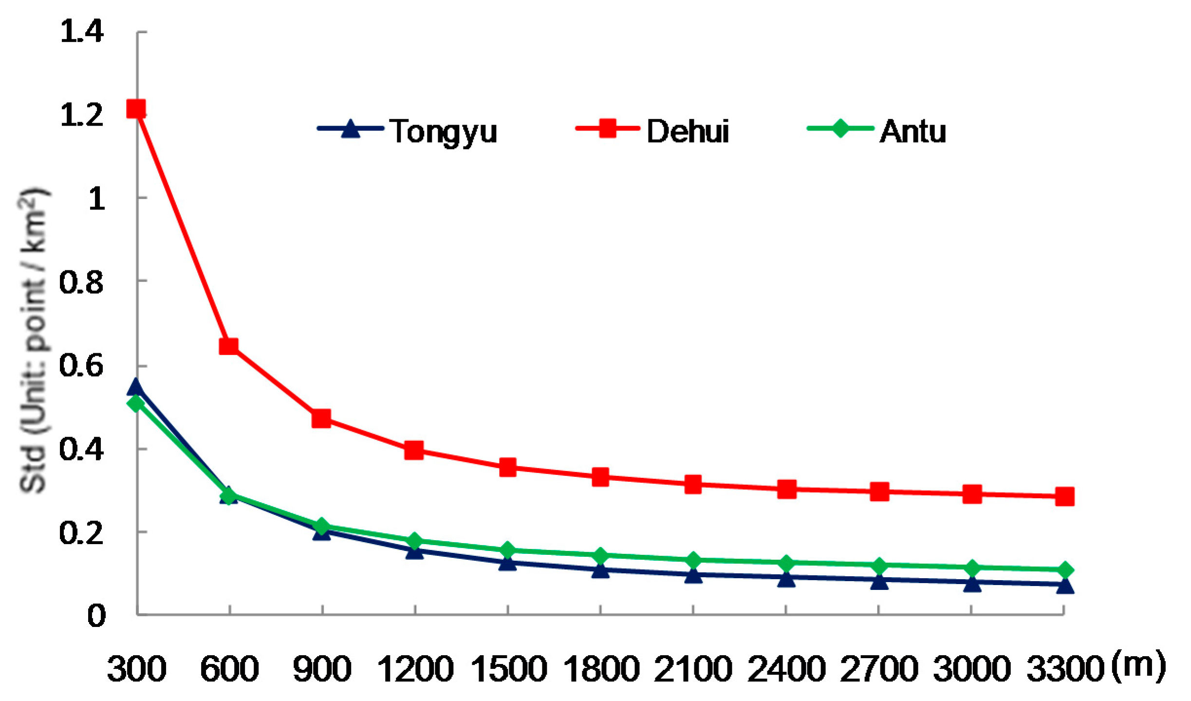
KDE was considered to be an effective method by which density is calculated using a kernel function superimposed over each location. The application of KDE requires the choice of the type of kernel function and the definition of three key parameters: bandwidth, cell size, and intensity [36]. Bandwidth is a very import parameter influencing the value of KDE. Increasing the bandwidth will not greatly change the mean of the density values calculated, but greatly affects standard deviations. The standard deviations of KDE for different bandwidths in the three counties were calculated (Figure 5), and the curve changed slightly when the bandwidth was approximately 2000 m. Therefore, a radius of 2000 m was selected to estimate the kernel density, and the results were divided into four levels.
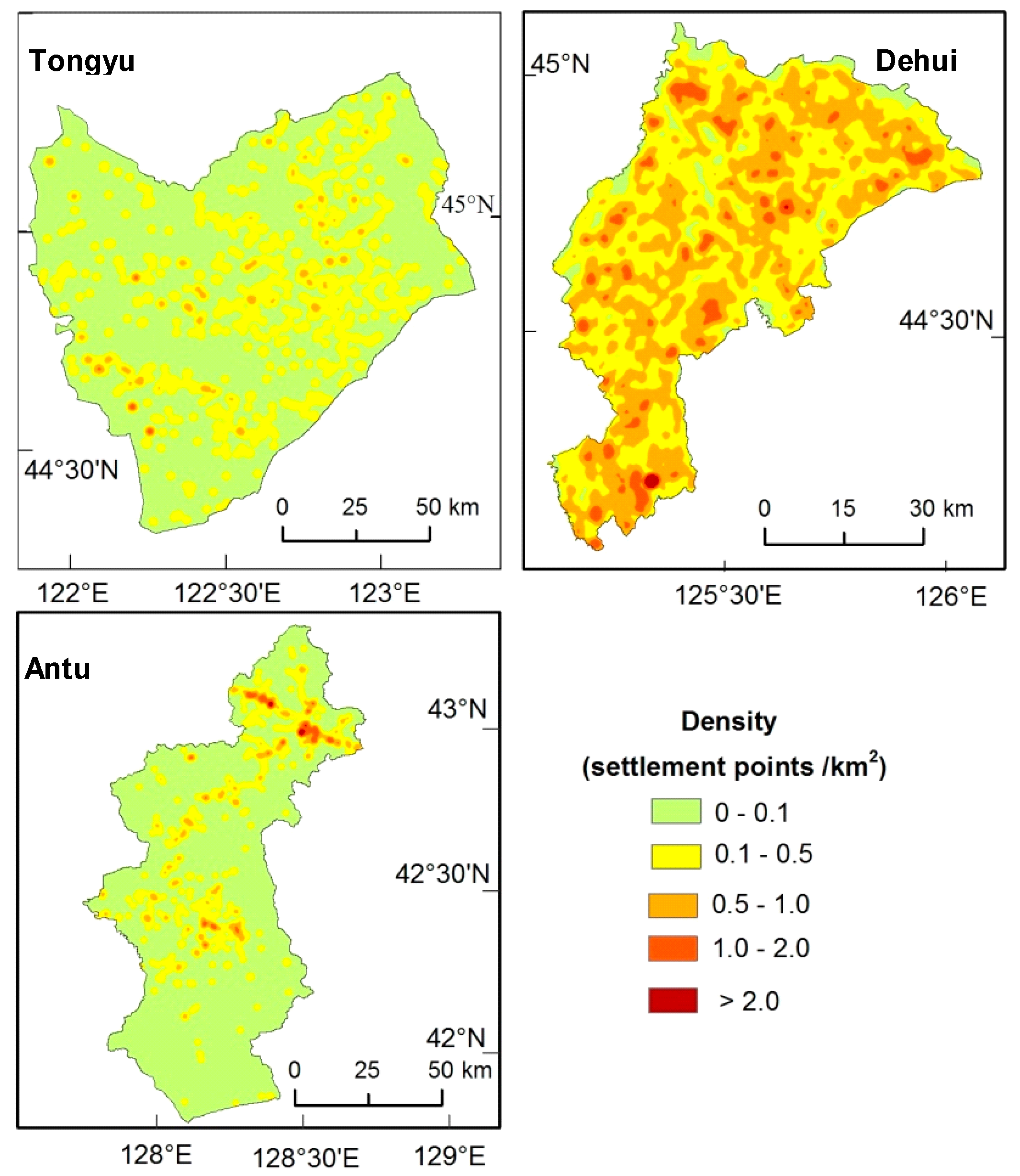
The mean values of the kernel density for Tongyu, Dehui, and Antu were 0.22, 0.32, and 0.21, and the standard deviations of KDE were 0.07, 0.26, and 0.11, respectively, showing that the settlement density of Dehui was larger, and the rural settlements in Tongyu were relatively uniform. The maps of KDE for the three counties looked very different (Figure 6). Influenced by the distribution of sandy land and salinized land, settlements distributed in Tongyu were sparse, and the density value was lower, especially in the northwest and southern parts (Figure 2 and Figure 6). There were many cluster centers in Dehui; therefore, the overall density value was higher. For Antu, the physical conditions in the mountainous area limited the distribution of rural residents, and the higher density values were presented as strips along the valley and main roads, leading to significant heterogeneity of the rural density.
3.2. Scale Distribution Characteristics of Rural Settlements
Three landscape indices, i.e., MPS, PSSD, and PSCV, and the Getis–Ord General G approach were employed to analyze the patterns of the scale distribution of rural settlements for these three counties (Table 2).
The MPS was 27.44 ha, 16.55 ha, and 10.08 ha for Tongyu, Dehui, and Antu, respectively, indicating the largest scale and lowest fragmentation of rural settlements in Tongyu. The PSSD of Antu was only 0.16, the smallest among the three counties, showing a largest landscape heterogeneity of rural settlements. We also calculated the PSCV for the three counties. We can see that the PSCV of Antu was larger than those of the other two counties, which indicates that the dispersion around the mean of the rural settlements in Antu was large.
Taking the area of rural settlements as the evaluated field, the clustering condition of high or low value was calculated by the Getis–Ord General G approach. The calculation results are shown in Table 3. We can see that the G(d) value of rural settlements in Tongyu and Antu was higher than the G(e) value, and their Z(G) values were all positive, indicating high value clustering for these two counties. The possibility of being influenced by a random process in these two counties was no more than 1%. For Dehui, the value of G(d) was equal to G(e), and the possibility that was influenced by a random process was 1.6%, showing there was no obvious phenomenon of gathering towers of large-scale settlements.
3.3. Morphological Characteristics of Rural Settlements
We used LSI and PCI as the qualitative metrics to compare the morphological difference of rural settlements (Table 2). The LSI measured the irregularity or complexity of the morphology of rural settlements. Among the three counties, the LSI of rural settlements in Dehui was the highest (the value was 78.43), and that of Antu was the lowest (the value was 39.69), showing that the morphology of rural settlements in Antu was regular and simple. The PCI value reflected the level of connection or continuity. The PCI of rural settlements for Tongyu was slightly higher (the value was 99.86) than that of the other two counties. The relatively higher PCI value indicated there were good connections and integration for settlements in Tongyu. The fragmented patches and disconnection of rural settlements decreased the value of the patch cohesion index of Antu.
3.4. GeographicAssociation
In terms of the spatial pattern of rural settlements, we learned that settlements in the three counties were all clustered. We analyzed the association between its pattern and geographic factors by landscape metrics. When the landscape metrics were used to characterize the rural settlement patterns, different features became apparent.
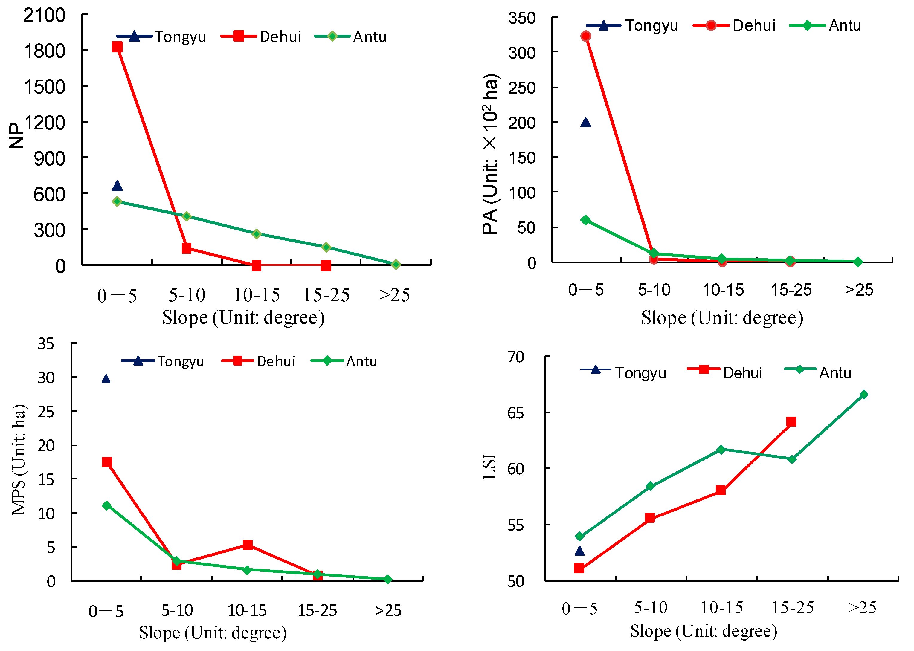
The influence related to terrain was obvious (Figure 7 and Figure 8). Due to the flat terrain and relatively small fluctuation, the influence of terrain was comparatively weak. All of the rural settlements were distributed within 200 m of elevation and a 5 degree slope, while the Tongyu settlements of Dehui were concentrated within 300 m elevation and 10 degree of slope, showing the opposite trend to terrain changes. Located in the mountainous area, the settlements of Antu represented obvious geographical differences. The number, area, and shape indices of settlements for Antu changed differently within and outside of the 800 m elevation range, showing a trend of rising first, and then decreasing. About 95% of the number and area were concentrated in the elevation range between 300 and 800 m. The number of patch (NP), patch area (PA), and MPS of Antu decreased when the slope increased.
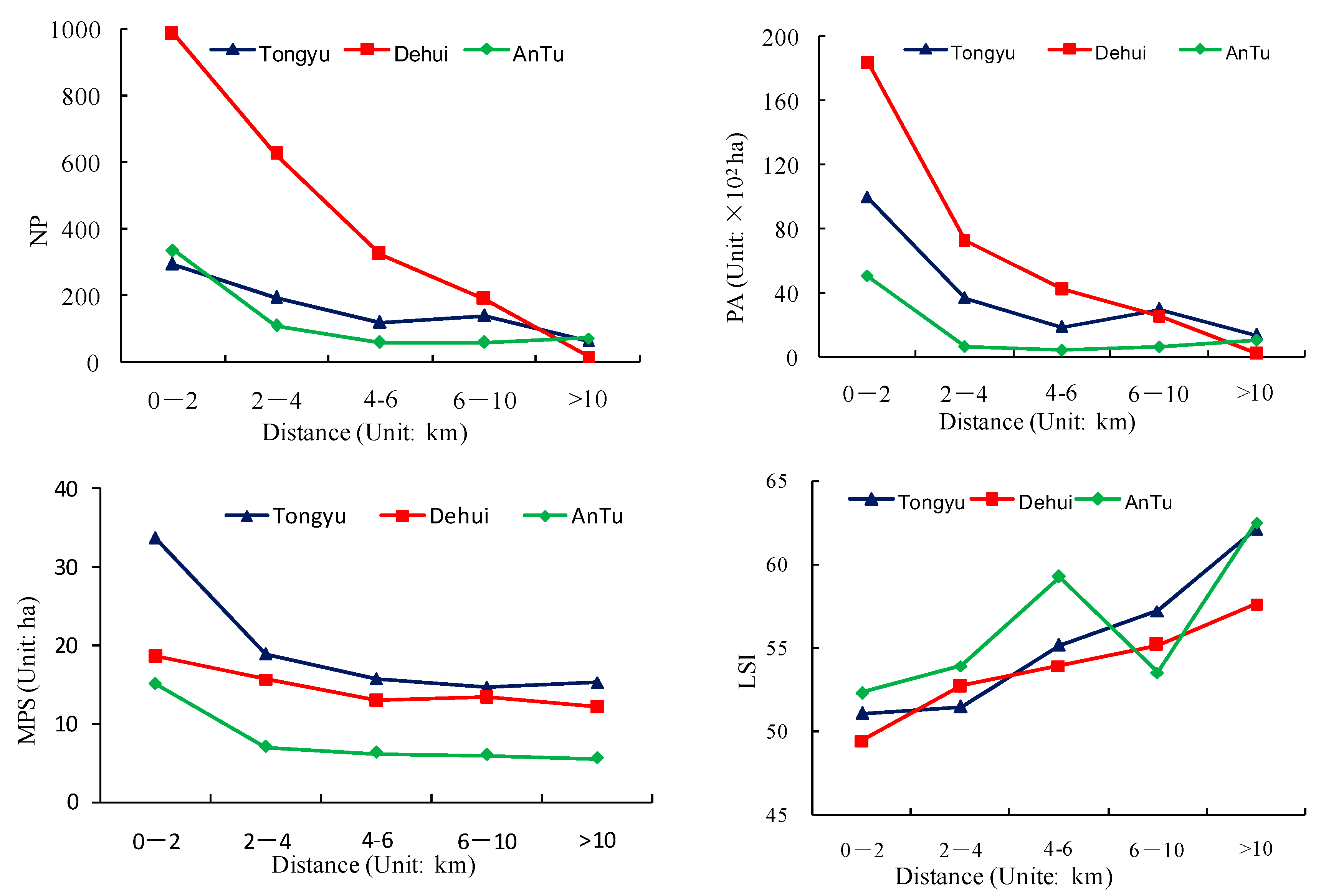
The influence brought by rivers is very complex (Figure 9). Theoretically, a water source is an important factor affecting the distribution of rural settlements in Tongyu because of the dry climate, but the number, area, and mean size of settlements increased when far away from the river. The number and area of settlements 6 km away from the river accounted for 79% and 77% of the total, respectively. For Dehui, the peak value for settlements distribution appeared in the 6–10 km distance range from the river, with the number and area decreasing within, or outside, of this distance. Compared with the settlement patterns of Tongyu, that of Antu showed a reverse trend, that is, the closer to the river, the more residents. The percentages of the number and area of settlements within 2 km of rivers were 50.16% and 69.58%, respectively.
When the landscape index was examined by road transects, we find that the curves of NP and PA for the three counties have similar downward trends when far away from the roads, while that of the LSI showed the opposite (Figure 10). The MPS of Tongyu was the highest among the three counties, and that of Dehui fluctuated slightly across the whole scale of the research.
The landscape shape index was quite variable across the three counties, with an opposite trend compared with NP, PA, and MPS analyzed by slope, proximity to rivers, and roads. A regional universal characteristic is that the greater the slope, the greater the index, and the farther away from the road, the greater the index.
In order to further analyzethe association between rural settlements and geographic factors, we conducted some correlation analyses between the settlement patterns and influencing factors at the test sites. In Tongyu, only the relationship between the settlement density and slope was statistically significant (Table 4; the total estimated settlement points in Tongyu was 666). The density of settlements in Dehui covaried positively with the elevation, slope, and proximity to water but covaried negatively with proximity to roads (the statistical number was 1793). For Antu (the statistical number was 581), the density of rural settlements was negatively correlated with DEM and the proximity to rivers and roads. The correlation coefficients were −0.411, −0.27, and −0.135 respectively, which was significant at the 0.01 level.
4. Discussion
This paper compared the spatial distribution patterns of rural settlements in different regions, and studied the relationships between the rural settlement distribution and DEM, slope, distance to river, and road. These aspects of the paper provide a valuable contribution to our understanding of geographic dependence on the human landscape, which count a great deal towards formulating rural community planning according to local conditions.
4.1. Spatial Pattern of Rural Settlements
We found that the density value in the middle part of Jilin province, typified by Dehui, was higher than the west and east parts of Jilin province because of substantially intensive agricultural use in this area. The west of Jilin province was one of the most important agricultural and livestock areas, but soil in this area was poor, and sandy land and salinized land were serious issues. The physical environment made a high density of rural settlements here impossible. For the eastern part, the physical conditions of the mountainous area limited the distribution of rural settlements, which brought a lower density and higher PSCV. The MPS of Tongyu (the value was 27.44 ha) was the highest among the three studied counties, even higher than the MPS of northeast China (the value was 21.46 ha [20]), indicating that the distribution of rural settlements tended to have a larger scale, but the larger PSSV showed a relatively large scale gap.
In terms of the spatial pattern of rural settlements, we found that settlements in the three counties were all clustered. This is good news from habitat conservation and countryside planning standpoints, because it limits habitat loss [37]. Still, settlement clusters were not randomly located, and occurred largely within close proximity to better amenities and good environments. For example, in Antu, more settlements were distributed close to rivers than farther away (Figure 9). This is troublesome, because there is intensive human activity in important ecosystems for many species that are easily damaged. Previous research studies also demonstrated that clustered settlements in artificial landscapes led to lower levels of habitat loss [37,38]. Therefore, our results suggested that not only the pattern of rural settlements, but also the location of the clustering, should be considered during conservation planning and countryside management. Thus, clusters must be located away from particularly sensitive and important habitats. In reality, the settlement patterns are very complex, and the measures seem to be more sensitive to the scale of analysis than what appears to be a centralized pattern to one better described as dispersed in other contexts [12].
Previous studies showed the rural settlements were agglomerated at a smaller scale (within 63 km [21]) or finer scale [37] when using Ripley’s K function. However, in our study, at the county scale, rural settlements showed clustering characteristics at a larger scale (over 100 km). We thought the results reflected the regional differences, to a certain extent.
4.2. Geographic Association
The clustering of settlements may result from many factors. The localized distribution of resources and the emergence of political or regional centers have often been highlighted [12]. In reality, the determinants varied because of the analytical resolution and the size and shape of the study area [12]. All of the factors can be divided into two types: physical factors and socioeconomic factors. The rural settlement patterns were the result of combined physical and socioeconomic factors [39]. Natural geographic conditions were the direct driving factor of the location and layout of rural settlements, while socioeconomic factors were considered decisive driving factors that determine the degree and speed of rural settlement development [40].
Among all of these factors, the terrain factors and river were taken as the leading physical factors [40]. Socioeconomic conditions, including traffic location, policies, the level of economic development, and the size and structure of the village population all have great influences on the layout and development of rural residential areas. As demonstrated by previous studies, the regional location of the rural settlements was determined by the influences exerted spatially outside of that site, e.g., the latitude, annual mean precipitation, annual mean temperature at a large scale, topography, and the distance to water and roads at a small scale [20]. Tian found that DEM, annual mean temperature, annual mean precipitation, and latitude were all factors influencing the distribution of rural settlements in northeast China [20]. On a county scale, the spatial pattern of rural settlements was more likely associated with terrain, proximity to water and roads, and agriculture suitability [41]. After referring to previous research results and the regional conditions, we selected DEM, slope, and distance to water and roads to capture the geographic associations with the distribution of rural settlements.
We found that there was obvious heterogeneity for geographic dependence on the human landscape. In our study, for example, settlement patterns of Tongyu were not determined predominantly by the proximity of neighbors, while those of Antu and Dehui were more closely correlated with physical factors. For Dehui, settlements were regularly distributed near the rivers, but were clustered far from them. This is very different from the river inclination of rural settlements in previous studies [37,41]. We speculate that due to the risk of flooding, settlements near the river were more sparse. However, for Antu, a mountainous county, more rural settlements were concentrated in the valley, within close proximity to the river. Dehui and Antu showed a closer relationship with physical factors, but represented different associations. All of these reflected the basis of the regional gradient of plain–hill–mountain.
Roadswere taken to be information landscape corridors between rural settlement landscapes, as well as between rural settlement landscape and other landscapes. Previous studies showed that there was significant positive correlation between transportation land areas and rural settlement areas [39,42]. On the one hand, with the economic developments, the distribution pattern of residential settlements directly affects the direction and flow of traffic lines. On the other hand, the distribution of traffic lines will change the spatial distribution of settlement structures.
More and more farmers prefer to dwell in the places that have convenient transportation [39]. In our study, the landscape indices of rural settlements in different buffer rangesnear roads were counted, and we found similar trends across the three counties: the closer to the road, the larger the number and area of rural settlements. However in Tongyu, correlation analysis showed that the correlation between rural patterns and road distance was not significant. According to the study results of Li [42], rural settlements and arable land showed an obvious symbiotic relationship. In Tongyu, land desertification and salinization changed the distribution pattern of arable land, and thus influenced settlement patterns, which represents the impact of agricultural suitability and the environmental adaptability of rural settlement patterns.
4.3. Distribution Pattern of Rural Settlements and Implications for Land Use Planning
According to the characteristics of the density, scale, and landform of rural settlements, we generalized three distribution patterns for the west, middle and east of Jilin province.
Pattern 1, represented by Tongyu, located in the west of Jilin province, is one of the most important agricultural and livestock areas. The physical environment for this region is characterized by flat alluvial plain, a semi-arid continental climate, lower precipitation, intensive evaporation, and poor soil conditions, resulting in serious desertification and salinization, and relatively low land productivity. The rural settlements in this region were relatively homogeneous and sparse, with obvious high-value clustering, indicting a larger scale. We labeled it the low-density, large-scale, and sparse type. For this type, we must fully consider the radiation of the regional center and ecological security, adjust the rural structure, and optimize the spatial layout. These goals can be realized by demolishing abandoned rural settlements and consolidating the scattered settlements.
Pattern 2, represented by Dehui, which is one of the major grain production bases in China, is located in the black soil zone, and has a relatively flat alluvial and diluvial platform, fertile soil, a better environment, and higher land productivity. Many people live here, and the density of rural settlements is higher. We labeled it the mass-like and point-scattered type. For this type, we should form a development pattern with multiple centers, adjust the scattered and extensive land use, tap the internal potential of rural settlements, utilize the land in an economical and intensive way, reclaim the abandoned homestead, and consolidate the rural settlements in an orderly fashion.
Pattern 3, represented by Antu, is called the Changbai mountain region, and is constituted by mountains and hills. Most of the scenery of this region is beautiful, so tourism has been developed. Limited by terrain, rural settlements in this region are centralized upon roads lying in the valley. The rural settlements were labeled as the low-density and high cluster-like type. For this type, we should improve the traffic conditions, strengthen the structure of public service facilities, make full use of the radiation effect of towns, and make reasonable planning and layouts for rural settlements.
5. Conclusions
In this research, we compared the regional differences of rural settlements by several methods, and explored the geographic associations of settlement patterns. Our study shows that the rural settlements in three counties were all clustered, but there are different characteristics in the aspects of concentration scale, distribution density, landscape morphology, and so on. Different geographic associations were the basis of the regional gradient of plain–hill–mountain. Three patterns of rural settlements representing characteristics of different regions were summarized, and measures were put forward according to the patterns. It is expected that the studied results will be useful for land use planning and the implementation of the regional policy of “building a new countryside”.
We should note that there are limitations of the study presented in this paper. For example, the results we obtained were restricted to the spatio-temporal scale of the data; the geographical determinants associated with spatial patterns we considered were only at a regional scale, and over one year. In addition, the study is static, and the settlement development over time was not taken into account. We used only morphological data—the distance from road and water—to quantitatively analyze the spatial characteristics of rural settlements in the studied counties. Other determinants, including physical and social variables, such as geology, land use, land cover, climate variables, the distance to natural amenities, and hazards, should be considered in the future. Furthermore, it is important to understand how to couple social and economic factors to build optimal regulation models.
Acknowledgments
This work is supported by the Natural Science Foundation of China (No. 41671219) and the Regional Project: Comparative study on land use and geochemistry in global black soil zones (No. DD201601).
Author Contributions
Xiaoyan Li conceived and wrote the paper; Yingnan Zhang and Huiying Li analyzed the data; and Limin Yang analyzed and summed up the literatures concerned.
Conflicts of Interest
The authors declare no conflict of interest.
References
- Long, H.L.; Liu, Y.S.; Wu, X.Q. Spatio-temporal dynamic patterns of farmland and rural settlements in Su-Xi-Chang region: Implications for building a new countryside in coastal China. Land Use Policy 2009, 26, 322–333. [Google Scholar] [CrossRef]
- Woods, M. Rural Geography: Processes, Responses and Experiences in Rural Restructuring; Sage: London, UK, 2005. [Google Scholar]
- Wang, C.; Wu, H.; Xu, H.C.; Zheng, J.; Zhou, H. Analysis on characteristics and distribution pattern of settlement in river valley: A case study in Fuping County of Hebei Province. Sci. Geogr. Sin. 2010, 21, 170–176. (In Chinese) [Google Scholar]
- Huber, N.L. The role of land use planning in sustainable rural systems. Landsc. Urban Plan. 1998, 41, 83–91. [Google Scholar]
- Shoshany, M.; Goldshelger, N. Land-use and population density changes in Israel—1950 to 1990: Analysis of regional and local trends. Land Use Policy 2002, 2, 123–133. [Google Scholar] [CrossRef]
- Hammer, R.B.; Stewart, S.I.; Winkler, R.L.; Radeloff, V.C.; Voss, P.R. Characterizing dynamic spatial and temporal residential density patterns from 1940–1990 across the North Central United States. Landsc. Urban Plan. 2004, 69, 183–199. [Google Scholar] [CrossRef]
- Radeloff, V.C.; Hammer, R.B.; Stewart, S.I. Rural and suburban sprawl in the U.S. midwest from 1940 to 2000 and its relation to forest fragmentation. Conserv. Biol. 2005, 3, 793–805. [Google Scholar] [CrossRef]
- Manonmani, R.; Mary, G.; Suganya, D. Remote sensing and GIS application in change detection study in urban zone using multi temporal satellite. Int. J. Geomat. Geosci. 2010, 4, 339–348. [Google Scholar]
- Modica, G.; Vizzari, M.; Pollino, M.; Fichera, C.R.; Zoccali, P.; Di Fazio, S. Spatio-temporal analysis of the urban–rural gradient structure: An application in a Mediterranean mountainous landscape (Serra San Bruno, Italy). Earth Syst. Dyn. 2012, 3, 263–279. [Google Scholar] [CrossRef]
- Amy, K.; Hahs, M.; McDonnell, J. Selecting independent measures to quantify Melbourne’s urban–rural gradient. Landsc. Urban Plan. 2006, 78, 435–448. [Google Scholar]
- Theohald, D.M. Land use dynamics beyond the urban fringe. Geogr. Rev. 2001, 91, 544–564. [Google Scholar] [CrossRef]
- Andrew, B.; James, C. Multiscalar approaches to settlement pattern analysis. In Confronting Scale in Archaeology; Springer: Boston, MA, USA, 2007. [Google Scholar]
- Kong, F.H.; Nakagoshi, N. Spatial-temporal gradient analysis of urban green spaces in Jinan, China. Landsc. Urban Plan. 2006, 78, 147–164. [Google Scholar] [CrossRef]
- Andrén, H.; Delin, A.; Seiler, A. Population response to landscape changes depends on specialization to different landscape elements. Oikos 1997, 1, 193–196. [Google Scholar] [CrossRef]
- Guo, X.D.; Zhang, Q.Y.; Ma, L.B. Analysis of the spatial distribution character and its influence factors of rural settlement in transition-region between mountain and hilly. Econ. Geogr. 2012, 32, 114–120. (In Chinese) [Google Scholar]
- Long, H.L.; Li, Y.R.; Liu, Y.S. Analysis of evolutive characteristics and their driving mechanism of hollowing village in China. Acta Geogr. Sin. 2009, 64, 1203–1213. (In Chinese) [Google Scholar]
- Wang, C.X.; Yao, S.M.; Chen, C.H. Empirical study on ‘village-hollowing′ in China. Sci. Geogr. Sin. 2005, 21, 257–262. (In Chinese) [Google Scholar]
- Wu, Y.J.; Guo, F.; Zhang, S.W.; Zhang, Y.Z. The study on spatial pattern of urban and rural residential landuse in Jilin Province. J. Arid Land Resour. Environ. 2006, 1, 108–122. (In Chinese) [Google Scholar]
- Zhang, Z.H.; Xiao, R.; Ashton, S.; Wu, J.P. Spatial point pattern analysis of human settlements and geographical associations in eastern coastal China—A case study. Int. J. Environ. Res. Public Health 2014, 11, 2818–2833. [Google Scholar] [CrossRef] [PubMed]
- Tian, G.; Qiao, Z.; Zhang, Y. The investigation of relationship between rural settlement density, size, spatial distribution and its geophysical parameters of China using Landsat TM images. Ecol. Model. 2012, 231, 25–36. [Google Scholar] [CrossRef]
- Ma, X.D.; Qiu, F.D.; Li, Q.L.; Shan, Y.B.; Cao, Y. Spatial pattern and regional types of rural settlements in Xuzou city, Jiangsu Province, China. Chin. Geogr. Sci. 2013, 4, 482–491. [Google Scholar] [CrossRef]
- Robert, H. Describing and modeling rural settlements maps. Ann. Assoc. Am. Geogr. 1982, 2, 221–223. [Google Scholar]
- Zomeni, M.; Tzanopoulos, J.; Pantis, J.D. Historical analysis of landscape change using remote sensing techniques: An explanatory tool for agricultural transformation in Greek rural areas. Landsc. Urban Plan. 2008, 86, 38–46. [Google Scholar] [CrossRef]
- Chakraborty, J.; Armstrong, M.P. Exploring the use of buffer analysis for the identification of impacted areas in environmental equity assessment. Cartogr. Geogr. Inf. Syst. 2013, 3, 145–157. [Google Scholar] [CrossRef]
- Fletcher, R. Some spatial analyses of Chalcolithic settlement in Southern Israel. J. Archaeol. Sci. 2008, 35, 2048–2058. [Google Scholar] [CrossRef]
- Anderson, T.K. Kernel density estimation and K-means clustering to profile road accident hotspots. Accid. Anal. Prev. 2009, 41, 359–364. [Google Scholar] [CrossRef] [PubMed]
- Liu, X. Study on the Security of Grain Reserves in Northeast China. Ph.D. Thesis, Jilin University, Changchun, China, 2013. (In Chinese). [Google Scholar]
- Wang, C.Y.; Tang, J.; Li, Z.Y.; Mao, Z.; Wang, X. Driving force analysis of land use and land cover temporal-spatial change in the west of Jilin province. Ecol. Environ. 2008, 17, 1914–1920. [Google Scholar]
- Li, X.Y.; Zhang, S.W.; Wang, Z.M. Spatial variability and pattern analysis of soil properties in Dehui city, Jilin province. J. Geogr. Sci. 2004, 14, 503–511. [Google Scholar]
- Definiens, A.G. Definiens Professional 8.6 User Guide; Definiens A.G: Munchen, Germany, 2011. [Google Scholar]
- Lu, C.Y.; Wang, Z.M.; Li, L.; Wu, P.Z. Assessing the conservation effectiveness of wetland protect areas in Northeast China. Wetl. Ecol. Manag. 2016, 24, 381–398. [Google Scholar] [CrossRef]
- Ripley, B.D. The second-order analysis of stationary point processes. J. Appl. Probab. 1976, 13, 255–266. [Google Scholar] [CrossRef]
- Besag, J.E. Commentson Ripley’s paper. J. R. Stat. Soc. Ser. B 1977, 40, 193–195. [Google Scholar]
- McGarigal, K.; Marks, B. Fragstats—Spatial Pattern Analysis Program for Quantifying Landscape Structure; Forest Science Department, Oregon State University: Corvallis, OR, USA, 1994. [Google Scholar]
- Riitters, K.H.; O’Neill, V.; Hunsaker, C.T.; Wickham, J.D.; Yankee, D.H.; Timmins, S.P.; Jones, B.K.; Jackson, B.L. A factor analysis of landscape pattern and structure metrics. Landsc. Ecol. 1995, 10, 23–39. [Google Scholar] [CrossRef]
- Uuemaa, E.; Mander, Ü.; Marja, R. Trends in the use of landscape spatial metrics as landscape indicators: A review. Ecol. Indic. 2013, 28, 100–106. [Google Scholar] [CrossRef]
- Gonzalez-Abraham, C.E.; Radeloff, V.C.; Hawbarker, T.J.; Hamer, R.B.; Stewart, S.I.; Clayton, M.K. Patterns of houses and habitat loss from 1937 to 1999 in Northern Wisconsin, USA. Ecol. Appl. 2007, 17, 2011–2023. [Google Scholar] [CrossRef] [PubMed]
- Odell, E.A.; Theobald, D.M.; Knight, R.L. Incorporating ecology into land use planning-the songbirds’ case for clustered development. J. Am. Plan. Assoc. 2003, 69, 72–82. [Google Scholar] [CrossRef]
- Jiang, G.H.; Zhang, F.R.; Qin, J. Relationship between distribution changes of rural residential land and environment in mountainous areas of Beijing. Trans. CSAE 2006, 22, 85–92. [Google Scholar]
- Gude, P.H.; Hansen, A.J.; Rasker, R.; Maxwell, B. Rates and drivers of rural residential development in the Greater Yellowstone. Landsc. Urban Plan. 2006, 77, 131–151. [Google Scholar] [CrossRef]
- Min, J.; Yang, Q.Y.; Weng, C.Y. The analysis of spatial distribution and optimization on rural settlement based on villageregion. Chin. Agric. Sci. Bull. 2012, 28, 283–290. [Google Scholar]
- Li, D.M.; Wang, D.Y.; Li, H. The effects of rural settlement evolution on the surrounding land ecosystem service values: A Case Study in the Eco-Fragile Areas, China. ISPRS Int. J. Geo-Inf. 2017, 6, 49. [Google Scholar] [CrossRef]
Figure 1.
Location of the study area.

Figure 2.
Land use maps of Tongyu, Dehui, and Antu.
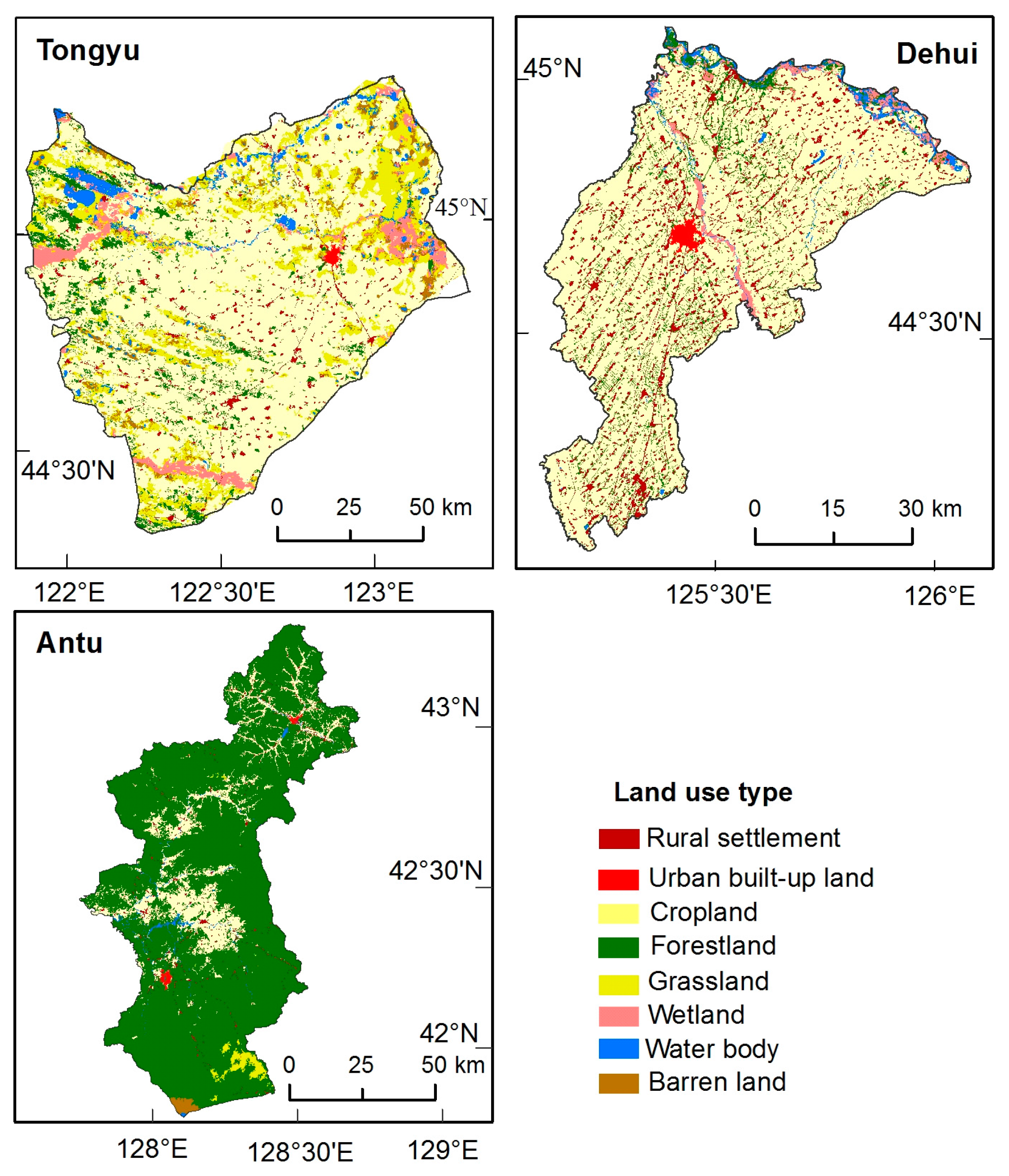
Figure 3.
Illustration of the kernel density method.

Figure 4.
Ripley’s K curves of rural settlements in the three counties.

Figure 5.
Standard deviations of kernel density estimation (KDE) for different bandwidths in the three counties.
Figure 5.
Standard deviations of kernel density estimation (KDE) for different bandwidths in the three counties.

Figure 6.
Map of kernel density in the three counties.

Figure 7.
Changes of the landscape indices with elevation.
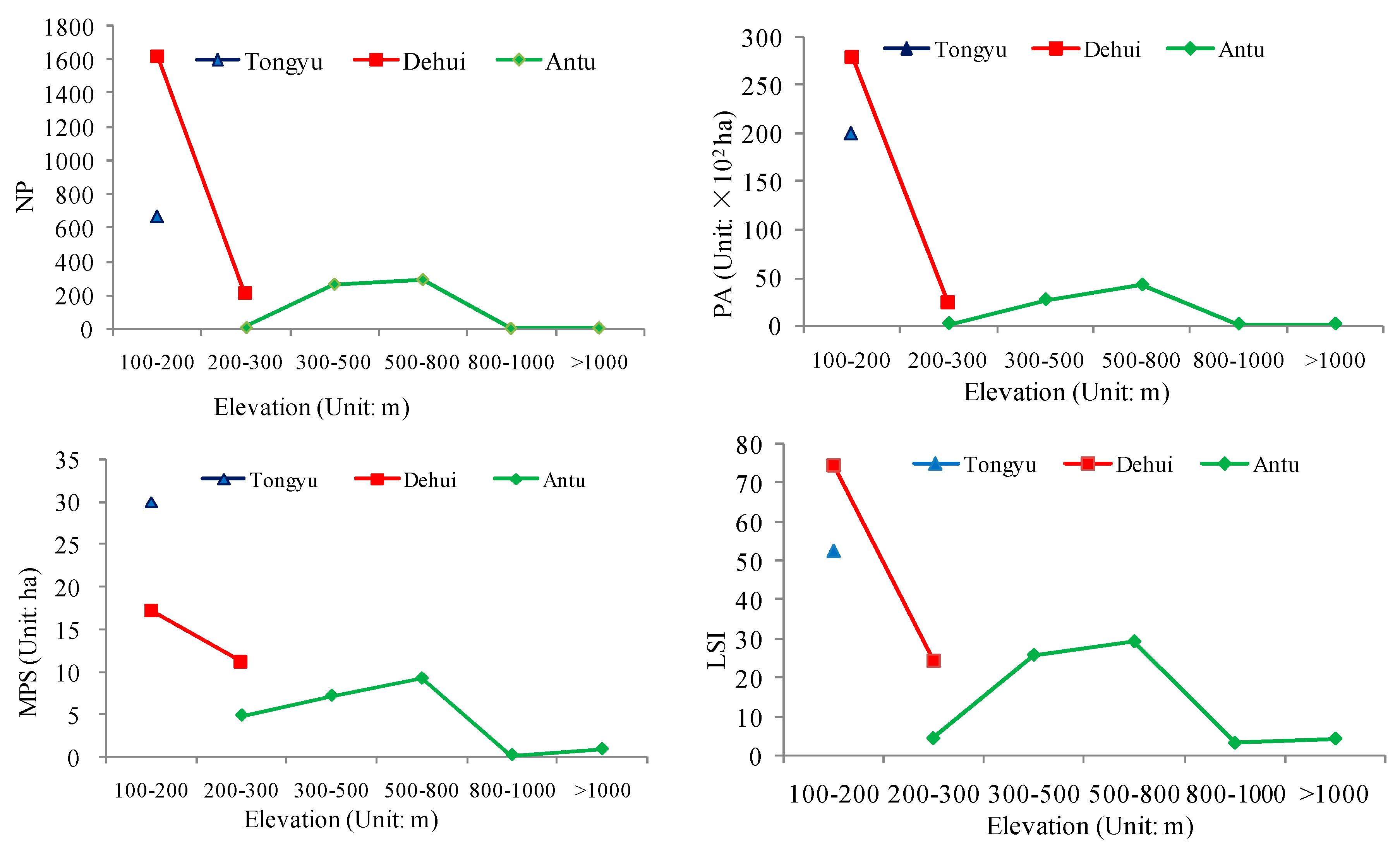
Figure 8.
Changes of the landscape indices with gradient.

Figure 9.
Changes of landscape indices with distance from rivers.
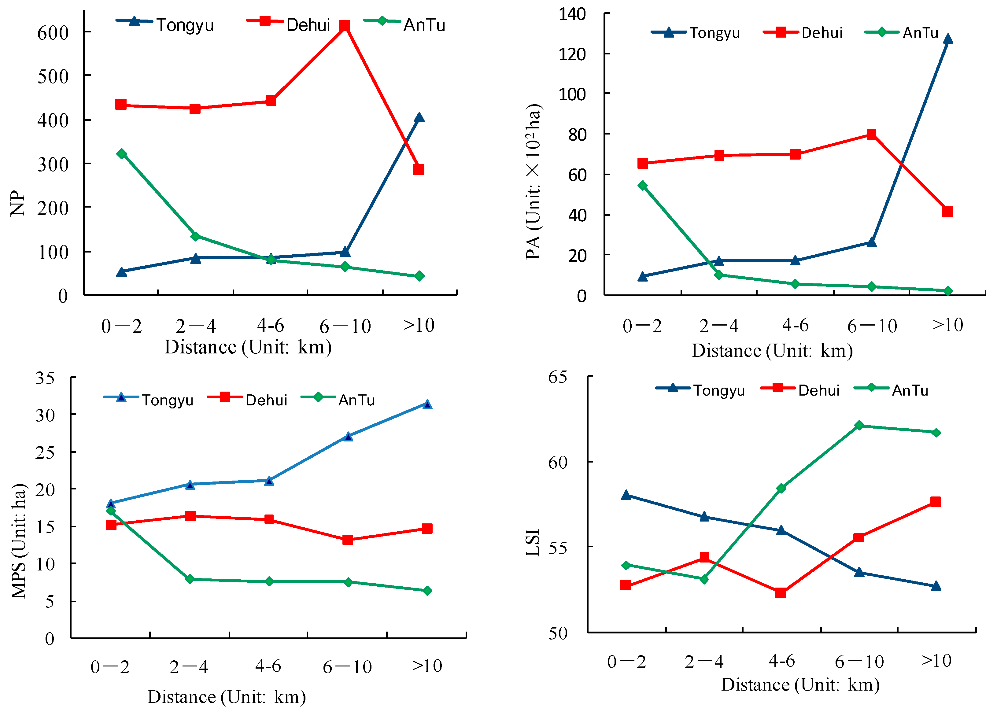
Figure 10.
Changes of landscape indices with distance from roads.


Table 1.
The formula and description of the indices.
| Landscape Metric | Abbreviation | Description | Unit |
|---|---|---|---|
| Average Nearest-Neighbor Index | ANN | . where di is the distance between two rural points; A is the total area of the landscape, and N is the total number of patches. | m |
| Mean Patch Size | MPS | . where A is the total area of the landscape and N is the total number of patches. | ha |
| tch Size Standard Deviation | PSSD | The standard deviation of patch size in the entire landscape. where A is the total area of the landscape and N is the total number of patch edges, aij is the area of path ij. | ha |
| Patch Size Coefficient of Variation | PSCV | The standard deviation of patch size divided by mean patch size for the entire landscape. × 100 | % |
| Landscape Shape Index | LSI | A modified perimeter-area ration of the form: , where E is the total length of patch edges and A is the total area of the landscape. | unitless |
| Patch Cohesion Index | PCI | PCI = × 100, where pij is perimeter of habitat patch ij, aij is area of patch ij, and A is total of the landscape. | unitless |
| Number of Patch | NP | ≥1, Equals the number of patches in the landscape. | unitless |
| Pach Area | PA | ≥0, Equals the area of patches in the landscape. | ha |
Table 2.
Landscape metrics of rural settlements in the studied area.
| Distribution of Rural Settlements | Scale of Rural Settlements | Form of Rural Settlements | ||||
|---|---|---|---|---|---|---|
| ANN | MPS | PSSD | PSCV | LSI | PCI | |
| Tongyu | 0.72 | 27.44 | 0.42 | 154.79 | 55.04 | 99.86 |
| Dehui | 0.84 | 16.55 | 0.25 | 153.71 | 78.43 | 99.82 |
| Antu | 0.51 | 10.08 | 0.16 | 161.20 | 39.69 | 99.78 |
Table 3.
Estimation of Getis–Ord General G for rural settlements.
| County | G(d) | G(e) | Z(G) | p |
|---|---|---|---|---|
| Tongyu | 0.000009 | 0.000008 | 4.4177 | 0.000010 |
| Dehui | 0.000007 | 0.000007 | 1.3992 | 0.016176 |
| Antu | 0.000059 | 0.000033 | 19.1667 | 0.000008 |
Table 4.
Correlations between settlements density and influencing factors.
| DEM | Slope | Proximity to Rivers | Proximity to Roads | |
|---|---|---|---|---|
| Tongyu | 0.028 | 0.087 * | 0.03 | 0.013 |
| Dehui | 0.139 ** | 0.071 ** | 0.206 ** | −0.104 ** |
| Antu | −0.411 ** | 0.009 | −0.270 ** | −0.135 ** |
** Means correlation was significant at the 0.01 level (bilateral). * Means correlation was significant at the 0.05 level (bilateral).
© 2017 by the authors. Licensee MDPI, Basel, Switzerland. This article is an open access article distributed under the terms and conditions of the Creative Commons Attribution (CC BY) license (http://creativecommons.org/licenses/by/4.0/).
Share and Cite
MDPI and ACS Style
Li, X.; Li, H.; Zhang, Y.; Yang, L. Spatial Patterns and the Regional Differences of Rural Settlements in Jilin Province, China. Sustainability 2017, 9, 2170. https://doi.org/10.3390/su9122170
AMA Style
Li X, Li H, Zhang Y, Yang L. Spatial Patterns and the Regional Differences of Rural Settlements in Jilin Province, China. Sustainability. 2017; 9(12):2170. https://doi.org/10.3390/su9122170
Chicago/Turabian StyleLi, Xiaoyan, Huiying Li, Yingnan Zhang, and Limin Yang. 2017. "Spatial Patterns and the Regional Differences of Rural Settlements in Jilin Province, China" Sustainability 9, no. 12: 2170. https://doi.org/10.3390/su9122170
Note that from the first issue of 2016, this journal uses article numbers instead of page numbers. See further details here.