The Role of Sustainable Investment in Climate Policy
by
Franziska Schütze
1,*, 
Steffen Fürst
1,
Jahel Mielke
1,2,
Gesine A. Steudle
1,
Sarah Wolf
1 and
Carlo C. Jaeger
1,3,4 1
Global Climate Forum, 10178 Berlin, Germany
2
Faculty of Economics and Social Sciences, University of Potsdam, 14469 Potsdam, Germany
3
State Key Laboratory of Earth Surface Processes and Resource Ecology, Beijing Normal University, Beijing 100875, China
4
School of Sustainability, Arizona State University, Tempe, AZ 85287, USA
*
Author to whom correspondence should be addressed.
Sustainability 2017, 9(12), 2221; https://doi.org/10.3390/su9122221
Submission received: 25 October 2017
/
Revised: 25 November 2017
/
Accepted: 26 November 2017
/
Published: 1 December 2017
(This article belongs to the Section Economic and Business Aspects of Sustainability)
Abstract
:Reaching the Sustainable Development Goals requires a fundamental socio-economic transformation accompanied by substantial investment in low-carbon infrastructure. Such a sustainability transition represents a non-marginal change, driven by behavioral factors and systemic interactions. However, typical economic models used to assess a sustainability transition focus on marginal changes around a local optimum, which—by construction—lead to negative effects. Thus, these models do not allow evaluating a sustainability transition that might have substantial positive effects. This paper examines which mechanisms need to be included in a standard computable general equilibrium model to overcome these limitations and to give a more comprehensive view of the effects of climate change mitigation. Simulation results show that, given an ambitious greenhouse gas emission constraint and a price of carbon, positive economic effects are possible if (1) technical progress results (partly) endogenously from the model and (2) a policy intervention triggering an increase of investment is introduced. Additionally, if (3) the investment behavior of firms is influenced by their sales expectations, the effects are amplified. The results provide suggestions for policy-makers, because the outcome indicates that investment-oriented climate policies can lead to more desirable outcomes in economic, social and environmental terms.
1. Introduction
In climate policy debates, a widespread assumption is that effective climate policy comes at substantial initial costs, and that therefore it would be a burden and a risk for producers and consumers alike. This understanding is at least partially attributable to the models behind it, which usually exclude positive effects by construction [1]. These models focus on marginal changes around an equilibrium that is Pareto optimal, except for climate damages in a more or less distant future. However, a sustainability transition typically implies a non-marginal transition from one economic equilibrium to another. Thus, a sustainability science approach differs from the standard economic approach, assuming, e.g., more complex interactions between the macro- and the micro-level [2].
A concept that relates to the recent macroeconomic discourse, which refers to a transition between different economic equilibria, is the idea of green growth. Jänicke et al. [3], Wolf et al. [1] and Pollin [4] provide more in-depth discussions on green growth and the green economy. However, only few studies have investigated short-term economic benefits of climate policy [5,6] or interaction effects between environmental regulation and technical progress [7]. Related reports from international institutions such as the Organization for Economic Cooperation and Development (OECD), United Nations Environmental Program (UNEP), the Worldbank, the World Economic Forum and others [8,9,10,11] usually do not use the same models as used in macroeconomic climate policy analysis. Green growth is mainly described by narratives rather than by a trajectory that can be assessed with formal models. According to Antal and van den Bergh [2] a synthesis of sustainability thinking and macroeconomics still needs to be accomplished.
Since most standard economic models exclude the possibility of green growth by construction, there are two possible solutions in terms of economic modelling: Creating new types of models that differ from the usual approach of computable general equilibrium (CGE) models, like, e.g., agent-based models, or changing certain mechanisms in CGE models in order to overcome some of their intrinsic limitations. Without in any way dismissing the former, this paper aims at the latter.
GEM-E3 [12], the model used for this purpose is calibrated to the European economy and has been used for evaluating EU level climate policies numerous times. The current situation in Europe in the aftermath of the financial crisis is characterized by low levels of investment, growth and employment. This makes Europe an interesting case for the investigation of a new type of climate policy [13], focusing on economic benefits and the role of investment. Additionally, these insights can be helpful for the discussion on how to reach the recently agreed international 1.5 °C climate target.
Our paper relates to the vast literature and reports on climate policy evaluation providing cost-benefit analyses. The IPCC [14] suggests that the cost required to mitigate greenhouse gas (GHG) emissions to safe concentration levels (450 parts per million by volume (ppmv)) ranges from 1 to 3.7% of GDP by 2030 (compared to the baseline GDP). The OECD [15] estimates climate mitigation costs to be approximately 0.5% of GDP by 2030. According to these calculations, timely and globally concerted action would reduce the costs of GHG abatement [16]. Studies that investigate the reduction of EU level GHG emissions, such as the European Commission Impact Assessment Report [17] come to similar conclusions. Depending on the policy scenario, the costs of a 40% emission reduction scenario is estimated to lie between 0.1% and 0.45% of GDP by 2030 (compared to the reference scenario).
According to the Impact Assessment Report, the implementation of a carbon price in all sectors and the reuse of the revenues to reduce labour costs would reduce the economic costs of GHG abatement. The reported costs are usually measured by comparing a reference scenario without constraints with a counterfactual scenario that includes a GHG emission target as an additional constraint to the optimization. In this way, the outcome can only be as good as, or worse than, the reference scenario. Rosen and Günther [18,19] provide a more detailed review of the analytical approaches and assumptions used in the Fifth Climate Assessment (AR5) of the IPCC [14] and their shortcomings.
Some models of climate policy (see e.g., [20]) include the future benefits from avoiding climate damages and air pollution, where the proper discount rate of avoided future costs is a decisive parameter and is therefore often debated. Potential short-term economic benefits, such as increased technical progress, international competitiveness, a positive investment climate or other feedback effects are usually not examined. However, when investigating fast decarbonization possibilities, which becomes ever more important with a 1.5 °C climate target, the impact of large amounts of investment on innovation and spillover effects should not be neglected. A key question is whether GHG mitigation can bring about economic benefits, even when costs of climate change (damages) in the future are not taken into account. Wolf [1] provides a comprehensive overview of different modelling approaches that address positive economic effects and the mechanisms they depend on.
This paper will investigate three mechanisms which are considered important for positive effects of climate mitigation:
- Several studies argue that the transition to a low-carbon economy requires large additional investment, e.g., UNEP and IEA estimate the required additional investment at global scale to be $0.5 trillion annually by 2020 and $1 trillion annually by 2030, in order to reach the target of staying below 2 °C global warming [21]. This number would increase for a 1.5 °C target. However, academic literature on the effects of green investment programs is scarce. To address this research gap, we introduce an investment program and investigate its effects.
- Technical progress is often regarded as a key mechanism for reducing abatement costs. Wing [22] notes that computational models used to evaluate the costs and benefits of climate policy often treat technical progress as exogenous and invariant to climate policy, and therefore disregard the feedback effects involved. There is a variety of approaches for the endogenization of technical progress, from the original hypothesis on induced technical change (ITC) by Hicks [23] to directed technical change for climate change mitigation by Acemoglu [24]. Most commonly used approaches are the stock of knowledge approach (see e.g., [25]) and the learning-by-doing approach (see e.g., [26,27]). We introduce a simple learning-by-doing mechanism based on production levels.
- As pointed out by Wing [22], the endogenization of technical progress via learning-by-doing gives rise to multiple equilibria. With more than one possible equilibrium, the question of equilibrium selection arises, which causes problems in a general equilibrium framework. This problem can be described as a coordination problem (see e.g., [28,29]). To address this, we introduce a mechanism of adaptive expectations, in which investment decisions of firms are influenced by sales expectations in the specific sector.
Although there are numerous studies on the effects of endogenous technical progress by various scholars (see [22], for an overview), it usually has not been studied in combination with other model changes or policies, such as adaptive expectations or an investment program. We want to test whether an investment program combined with changes in the model mechanisms can trigger a shift from economic costs to benefits within the given model framework.
This paper is organized as follows: In Section 2, we first describe the standard CGE model and the default features of the modelling framework. Second, we describe the model mechanisms considered crucial in determining the overall economic impact of GHG mitigation, and especially key mechanisms for sustainable investment. Third, we provide a description of different scenarios, which are characterized by different combinations of policies and model changes. Section 3 compares the results of these scenarios and Section 4 summarizes the findings.
2. Materials and Methods
The objective of this work is to discuss crucial mechanisms for a more comprehensive economic evaluation of climate policies that foster investment.
2.1. Landscape
There are different modelling approaches, such as macro-econometric, computable general equilibrium or systems-dynamics, which are used to assess the economic impacts of alternative climate policies.
Computable general equilibrium (CGE) models are the most commonly used tools for the assessment of climate policy, since they simultaneously capture the interrelation of all markets and agents while allowing for the integration of alternative policy scenarios. All scenarios in these models represent an optimal allocation of resources under different types of constraints. By construction, the reference scenario represents a long-run equilibrium where the economy grows at a steady rate. Hence, all other scenarios lead to sub-optimal solutions within the given analytical framework.
CGE models, however, may fall short on realism as they do not capture market imperfections. However, several extensions to the classical Arrow-Debreu-type [30] of general equilibrium models have been made, to make them more realistic. Such extensions are involuntary unemployment in the labour market [31], oligopolistic competition and monopolies [32] and endogenous productivity [33]. This paper addresses additional mechanisms that are expected to play an important role for climate policy.
2.2. The GEM-E3 Model
This section provides an overview of the core structure and key mechanisms of the model used.
2.2.1. Model Description
For the purpose of this paper, a well-established computable general equilibrium (CGE) model, GEM-E3, is used. This description is based on the detailed model description of GEM-E3, which can be found in the GEM-E3 reference manual [12] and the GEM-E3 model documentation [34]. The model has been applied for policy analyses and impact assessments of climate policy, such as the Impact Assessment Report of the European Commission [17].
The GEM-E3 model is a macroeconomic recursive-dynamic CGE model with multiple regions and sectors. It consists of a CGE core and an environmental module. Different versions of the model can differ regarding their characteristics, such as varied closure rules and institutional regimes. The environmental module includes emission permits, energy efficiency standards and several policy options for allocating emission permits and for using the generated revenues. Labour, (total factor) productivity and expectations on sectoral growth rates are the main determinants of economic growth.
The main characteristics of the model are:
- Firms: Firms operate under perfect competition and use a nested production function, including capital, labour, energy and materials. Firms are characterized by myopic expectations.
- Households: Representative households (one for each country and region) maximize a utility function to determine their demand for goods and services. The household can buy durable (equipment) goods, non-durable (consumable) goods, and services. The use of durable goods requires some amounts of non-durable goods.
- Markets: Firms optimize their profits and households optimize their utility, determining supply and demand for goods and services. Equilibrium prices are derived in the market, by ensuring that supply equals demand. Consumption and investment are allocated using transition matrices.
- Technology: Technical progress is exogenously represented in the production function. In each time step, the producer can change its production inputs depending on changes in prices of labour, capital and all intermediate goods and services. The electricity sector is more detailed, differentiating between different technologies producing electricity.
- Externalities: Greenhouse gas emissions are included as an environmental externality by introducing an additional constraint on the system. The emission constraint produces a shadow price for the emissions. Firms can invest in pollution abatement capital, which reduces emissions per unit of output, and hence its costs. This version of the model does not include damages to the environment and the economy in the future.
- Output: Projections are made in 5-year intervals and include macroeconomic output (investment, capital, consumption, employment, balance of payments, input-output-tables, and others) as well as output related to energy and the environment (energy use and supply, greenhouse gas emissions, pollution permits, pollution abatement capital).
Appendix A provides a short technical description of GEM-E3-M50, the version of the model used for this paper, as also presented in Jaeger et al. [6].
2.2.2. Investment and Related Mechanisms
The hypothesis to be tested in this paper, is that investment is a key mechanism for producing positive economic effects of climate policy. In order to test this hypothesis, it is necessary to determine the variables that are inputs to and outputs of investment from the investment function in GEM-E3 (as shown in Formula (6) below):
- Inputs to investment: The investment demand is endogenously specified using Tobins’Q [35], by comparing the market price of capital with its replacement cost. In the current implementation, investment depends on: the optimal demand for capital (given by the production function and elasticities), the depreciation rate (technologically determined), the interest rate (arising from financial market dynamics which are outside the scope of the model), the unit cost of investment, expectations on sectoral growth (exogenously defined), as well as a calibrated scale parameter. We derived two main possibilities of influencing the investment decision:
- To change the unit cost of investment via an investment subsidy
- To endogenize expectation dynamics, such that investors learn from their past experience.
- Outputs of investment:
- Technical progress is exogenous in the model at hand. In the real-world, however, investment has an influence on technical progress - therefore this mechanism will be addressed.
- Investment influences the size of the capital stock and through that production and employment. Its effect is the substitution of labour with capital and between different types of capital - leading to higher unemployment and crowding-out of investment as a first-round effect (which is then offset through higher production levels as a second-round effect). This is an issue we will investigate in the simulation results.
The key mechanisms which will be investigated further in Section 2.3 are: the effects of an investment subsidy, expectation dynamics and technical progress.
2.2.3. GHG Emissions Constraint
A standard way of introducing climate targets is in the form of a policy that puts a cap on total emissions allowed, hence an additional constraint is added to the optimization problem. In this case, we have chosen a more ambitious climate target than the one agreed in the European Union (40% by 2030 compared to 1990), namely 50% (the respective scenario is called M50 only, as described in Section 2.4). Simulations for the Impact Assessment Report [17] have shown that applying a 40% GHG emission reduction target leads to small negative effects on GDP between 0.1% and 0.45% by 2030 (compared to the reference scenario).
To give a structured overview of the model changes and expected outcomes, we formulate a number of propositions. Proposition 1 is used in combination with the model extensions but is based on an existing mechanism in the model.
Proposition 1.
The introduction of an emission cap in the form of an additional constraint to the optimization problem, will lead to a worse economic outcome.
2.3. Relevant Mechanisms and Related Model Extensions
This section describes the model changes implemented to account for the mechanisms described in Section 2.2.2 . The propositions are used to structure the model changes and the expected results based on the mechanisms of general equilibrium models in general and the GEM-E3 model in particular.
2.3.1. Investment Program
A key goal of this paper is to evaluate the effects of a considerable increase in low-carbon investment (public or private) in addition to the introduction of a GHG emission cap.
Greening the economy is the target of a number of green recovery proposals (e.g., [36,37,38,39]), notably the Green New Deal proposed by the European Green Party (e.g., [40]) and The New Climate Economy Report [10]. They highlight the large scale and long-term benefits, such as “building the foundations of sound, sustainable and strong growth in the future” [36]. Two channels through which public expenditures can be geared towards a green economy are proposed by UNEP’s Green Economy Report: redirecting public investment and greening public procurement [8]. Further, increasing the leverage effect of public investment on private investment is being discussed at different levels, national, EU and international. UNEP’s Green Economy Report suggests government actions that set conditions for private investment: to phase out fossil fuel subsidies, to reform existing incentives and provide new incentives, and to strengthen market-based mechanisms [8].
The World Economic Forum [9] concludes that 80% of investment will have to come from private sources. Zenghelis et al. (see [38,41,42]) analyse the possibility of stimulating additional net private sector investment in detail. Finding historically low investment levels in most OECD countries, the authors see a “lack of confidence to invest rather than a lack of liquidity” [42] and argue that credible long-term green growth policies provide opportunities for restoring confidence and leveraging additional investment [41]. Similarly, the Green Economy Report calls for the private sectors’ “understanding and sizing the true opportunity represented by green economy transitions across a number of key sectors” [8].
A key assumption of CGE models, however, is full employment of resources. Under this assumption, any new investment project will reduce investment elsewhere. This crowding-out effect is a key distinction between optimizing and non-optimizing models. If increasing investment levels improves the economic situation, this can either point to the fact that there is another possible equilibrium point, which actors cannot foresee or cannot coordinate on. Or it points to the fact that there are market imperfections in place that lead to a non-optimal outcome in the current situation.
To represent this mechanism in the model, a green investment program was introduced. For the purpose of this paper, the investment program was modelled as a change in policy. The value-added tax (VAT) is increased and the resulting additional revenues are used to subsidise investment. It is important to note that, what we want to investigate is the effect of the investment program and not how the additional investment is funded. The way it is implemented is comparable to other reallocation policies, such as the introduction of a price on carbon or a cap on the maximum amount of carbon emissions. Therefore, it can be expected that it leads to a crowding-out effect.
The required additional VAT is calculated such that the government revenues are increased by 10% compared to the reference case plus the GHG emission constraint (the scenario M50 only). Hence, the new VAT revenues are determined by:
where “Ref” denotes the reference scenario, “M50only” the 50% GHG emission reduction scenario and “Cf” denotes the counterfactual scenarios, meaning the “M50only” scenario with additional model changes.
The subsidy per unit of investment, , is calculated such that the new investment is equal to the M50 only investment plus the additional value-added tax (VAT) revenues:
with being a negative value.
Proposition 2.
In a standard CGE model, such as GEM-E3, an investment program leads to an outcome that is worse than the scenario it is based on (M50 only), because it reallocates resources away from the optimal allocation.
Proposition 3.
If the reference scenario is the optimal scenario by assumption, an investment program will always lead to crowding-out of consumption by investment (and of investment in one sector by investment in another) in the short-run.
2.3.2. Learning by Doing
CGE models, apart from few exceptions which will be described below, represent technical progress exogenously. However, the technical progress of clean technologies is key for a transition to a low-carbon economy. A considerable increase in low-carbon investment will increase the production level of these sectors. This will increase technical progress for these products through product and process innovation. An exogenous rate of technical progress does not take this feedback effect into account when higher levels of investment are applied.
Wing [22] differentiates four ways of introducing technical progress endogenously, two of which are used less often: (1) price-induced input augmentation and (2) backstop-technologies; and two of which are more popular: (3) the stock of knowledge approach and (4) the learning-by-doing approach.
Price-induced input augmentation is not used very often, due to difficulties in specifying a function that describes the relation between relative input prices and the augmentation of different inputs. Backstop-technologies are regarded as a semi-endogenous approach, which allows for radical technical change by introducing a new production technique. The new technique will be employed in response to an increase in prices, which in turn is dependent on other variables, mostly exogenous.
The stock of knowledge approach results from the new economic growth literature, where knowledge is represented as a kind of capital, the stock of knowledge (H), which grows with R&D investment, depreciates over time and follows an innovation process (transformation function)—which includes the efficiency of innovation, diminishing returns to R&D and spillover effects. However, the problem is the lack of disaggregated data on R&D and the calibration of initial knowledge stocks. The central argument is that climate policy does not increase R&D in general but that there is a trade-off between innovation (accumulation of knowledge) in different sectors. Popp [25] and related papers implement a stock of knowledge approach into the DICE model. Furthermore, Acemoglu and colleagues [24] use a stock of knowledge approach as well and find that a combination of carbon taxes and (temporary) research subsidies is sufficient to redirect technological development towards clean technologies through investment.
In the learning-by-doing (LBD) approach, the key parameter is the learning rate which depends on experience in a given sector. See Arrow [43] for a discussion on which economic variables are a good proxy for experience. Bottom-up models favor the LBD approach and mostly use cumulative capacity or cumulative production levels as a proxy for experience. Grubb [27] use cumulative abatement as a proxy. There is a rich literature on learning and experience curves, which started with a study by Wright [44] who introduced the concept of “learning curves”, measuring learning-by-doing as labour cost reduction in relation to cumulative output. He found a constant percentage of unit labour cost reduction per doubling of cumulative output in airframe manufacturing. Later on, the concept was extended to “experience curves”, by including different learning effects through R&D, production scale, cost of capital, etc. and by investigating total product costs instead of labour costs. Nagy et al. [45] compare three different “laws” of technical progress (time, production levels and cumulative production) for a large set of technologies and find that all three show very similar development paths for a large set of technologies. However, it is not straightforward to transfer these micro-level learning curves to the macroeconomic level.
The goal here is not to build on the vast amount of literature on technical progress by providing deeper insights into the forces that drive it. Instead, we start from the point that technical progress is present and is linked to the “experience” in a sector. Hence, exogenous learning parameters which do not change in response to policy induced changes in sectoral compositions, miss an important part of the feedback effects triggered by climate policy.
In the model used, technical progress or total factor productivity is determined by calibrating the model to exogenously given GDP growth rates. This is done because the purpose of the model is not to predict growth but to assume that under business as usual the official growth rate predictions (e.g., by DG ECFIN [46] in the EU) will be realized in the reference case.
In our approach we have semi-endogenised TFP in order to reflect learning by doing effects from higher production levels. The equation below describes the computation of TFP. It remains a calibrated parameter but an additional factor is added that depends on the production level:
where “i” denotes the sector, “j” denotes the region and“t” denotes the time. is the sum of the sectoral outputs over all regions j, i.e., because spill-over effects between different regions are important for technical progress. The correction factor shows that technical progress in a given sector increases when the production in that sector increases. This means that TFP stays the same in the reference case (as production does not change). However, different levels of production in the counterfactual scenarios lead to different levels of TFP.
The review by Wing [22] showed that a common way to prevent implausible market share dynamics in LBD approaches is to include upper bounds. In this paper we introduced an upper bound on the correction factor. Furthermore, for simplicity we assume that shrinking sectors do not “unlearn” immediately in response to reductions in demand. Hence, to prevent unreasonable dynamics, the correction factor is limited to a range from 1 to 3., i.e.,
Proposition 4.
The partial endogenization of learning-by-doing leads to an improvement of GDP as compared to M50 only, due to its effect on productivity.
Proposition 5.
The combination of learning-by-doing with an investment program leads to an improvement of GDP, because the investment program triggers a stronger learning-by-doing effect.
2.3.3. Expectations
The before mentioned literature suggests that technical progress creates positive externalities in the form of spillover effects, which can lead to underinvestment in these technologies. There are two main reasons for this: (1) the social benefit of innovation is higher than the private benefit of the individual investors (2) the benefit is often beyond the investment horizon of the individual.
Often, investors do not take into account their individual contribution to overall technical progress (because this depends on the behavior of others). Instead, they take it as given and collectively invest below the social optimum. Zenghelis [38] describes climate change as a market failure emerging from uncoordinated actions of individuals that leads to a collectively inferior outcome. Such a mechanism of expectation dynamics has already been investigated in Jaeger et al. [5,6]. If several producers invest more into their productive capital, they will experience higher overall technical progress. If this experience is taken into account in investment decisions in the next period, this can lead to positive expectation dynamics.
Investment connects two time steps in a model. Expectations about future prices, policies and demand are crucial in determining the return on investment (which is subject to uncertainty) and therefore, the investment decision. The latter then drives the optimal allocation of capital leading to the optimal outcome.
In the model used, time is modelled in a recursive dynamic way and agents have myopic expectations. Investment is described by the following function:
where is a calibrated scale parameter; K is the optimal demand for capital; is the cost of capital; is the cost of investment; d is the rate of depreciation; r is the national interest rate; is an exogenous parameter expressing expectations about sectoral growth. STGR represents the expectations on the future rate of capital return, to ensure that the investment plans are actually realized. Since STGR is an exogenous parameter calibrated to the reference scenario, it does not change with production levels (sales expectations of firms).
However, to include a response to increased rates of investment, this parameter should change endogenously, depending on the economic performance of that sector. For the purpose of better representing expectation dynamics, the following adjustment of STGR was implemented to represent adaptive expectations:
Similar to the correction factor described in Section 2.3.2, this represents the fact that sales expectations in a given sector depend on past experience: the larger the change in production level in that sector in a specific country, the higher the sales expectations for the next period and vice versa. The difference to Section 2.3.2 is that output values are differentiated by country and sector, , because for expectation dynamics we do not assume large spillover-effects between countries (larger sales in one country do not necessarily lead to higher sales expectations in another country). Furthermore, we assume expectations to be more responsive to increases in production than technical progress, which is why we assume a quadratic relationship.
In sectors with small output levels, the correction factor can lead to large adjustment of the STGR parameter. To take this into account, the correction factor is limited to a range from 0.5 to 3, allowing for negative effects on expectations as well, i.e.,
Proposition 6.
The partial endogenization of expectations does not lead to an improvement of GDP as compared to M50 only, as it amplifies the negative effects of the emission target through its effect on production levels.
Proposition 7.
The combination of all three mechanisms (adaptive expectations, learning-by-doing and an investment program) is expected to result in higher levels of GDP as compared to all other scenarios, because the three effects work in the same direction.
The next section describes the scenarios used for the analysis.
2.4. Scenario Description
For the purpose of testing the propositions, different scenarios are defined. The geographical focus is Europe, since the low levels of investment make it an interesting case for these specific model changes.
2.4.1. Reference Scenario (Ref)
The first step is to define a reference scenario, which represents the optimal growth path in the absence of any imperfections or frictions and assumes a business-as-usual world in terms of policies.
The data used for GEM-E3-M50 for the European Union consists of national accounts data and input-output tables from Eurostat. One underlying assumption of the reference scenario is that the output growth rate is in line with macro-economic projections, in this case 2012 Ageing Report prepared by DG ECFIN [46]. According to this report, the EU28 will have a growth rate of 1.5% over the period 2015–2050 and a decrease in the working age population. The methodology for the calibration of the exogenous parameters is described in more detail in the GEM-E3 model documentation [34]. Although the calibration of the reference scenario is not based on the latest data and projections, we do not consider this as problematic. This paper aims at identifying general mechanisms and focuses on the comparison of a reference scenario with counterfactual scenarios.
The different counterfactual scenarios are compared and evaluated against the reference scenario. A counterfactual scenario uses different assumptions (including changes in exogenous variables or policies). If these changes do not affect the reference scenario, the model does not need to be re-calibrated. The aim of the model changes introduced for the purpose of this paper is to keep the calibration of the reference case unchanged, to ensure comparability of results.
2.4.2. Climate Policy Scenario (M50 Only)
All assumptions are identical to the reference scenario for this scenario. Additionally, it includes a constraint on total greenhouse gas emissions. To show the impact of an “extreme” scenario, we chose a more ambitious emission reduction target than the currently agreed target of 40% (compared to 1990). For this scenario, we apply an emissions reduction target of 50% compared to 1990 (approx. 46% reduction from 2005). No changes in climate policies are assumed for non-EU countries. To exclude other reallocation effects, it is assumed that the carbon tax revenues are not reused in the economy for a specific purpose (although this is generally possible within GEM-E3) but they are used instead to improve the public budget.
2.4.3. Variants with Model Changes
To perform an evaluation of the effects of the mechanisms introduced into the model, several scenarios with different combinations of model changes have been analysed. The scenarios are specified in Table 1.
3. Results
3.1. Macroeconomic Aggregates
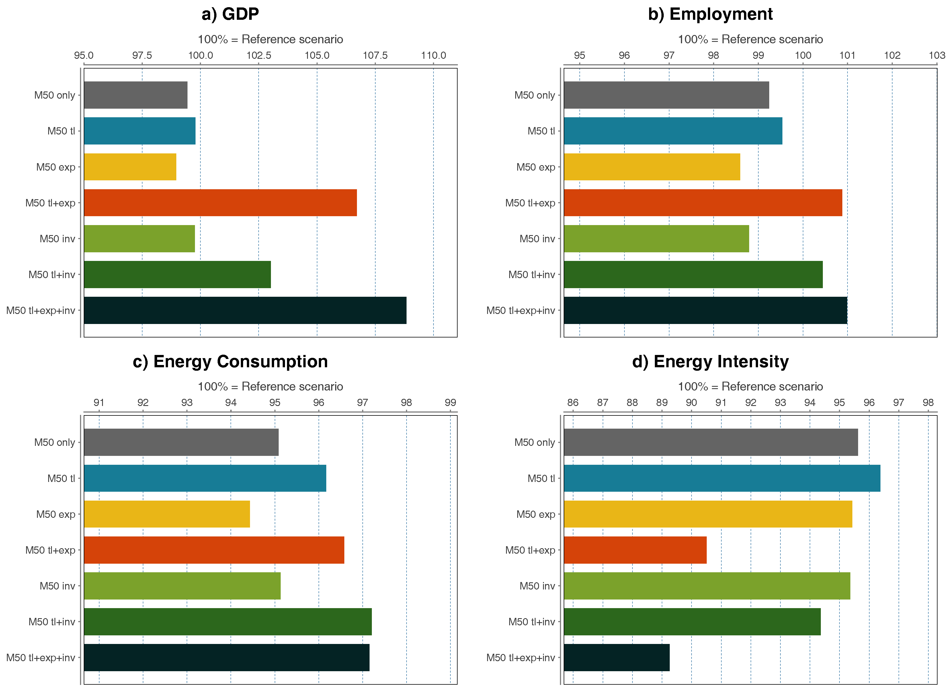
This section shows the main findings of the simulations. Table 2 shows the results of all scenarios compared to the reference scenario in 2030. For GDP, employment, and energy consumption and energy intensity, the results for 2030 are also depicted in Figure 1. Appendix B shows the main outcomes of the reference scenario. The combined scenario (M50 tl + inv + exp) performs best in all four dimensions.
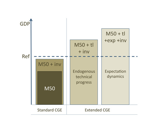
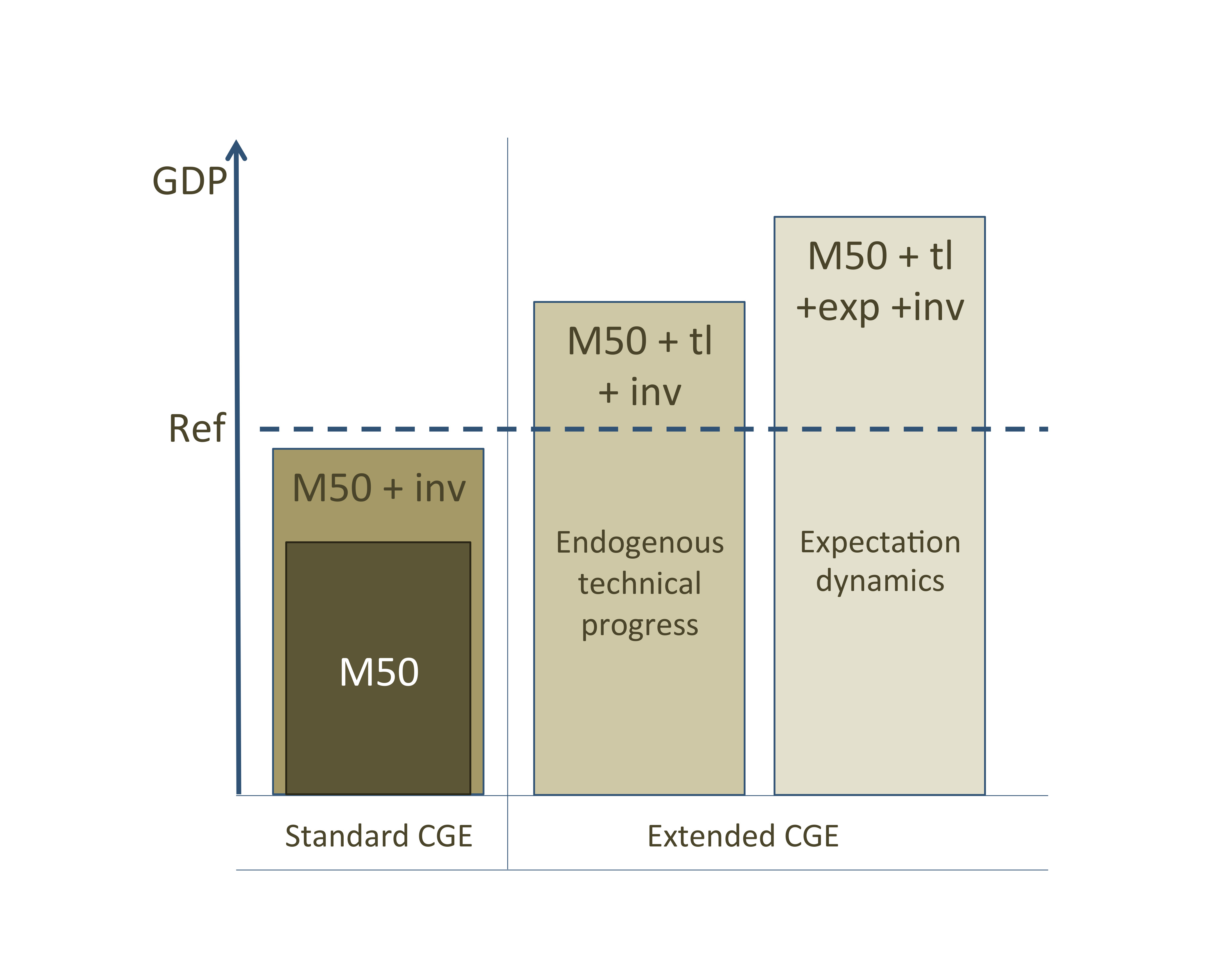
We can see that the M50 only scenario (with an ambitious climate target, but no model changes applied), shows a decrease in GDP compared to the reference scenario (−0.56% GDP in 2030 compared to reference) due to a 50% GHG emission reduction target. This corresponds with the results of the European Commission Impact Assessment Report on the 2030 climate and energy framework [17], showing GDP effects between −0.1% and −0.45% in 2030 when comparing a 40% emission reduction scenario with the reference scenario. This outcome supports Proposition 1.
M50 combined with the investment program (M50 inv) shows slightly improved GDP results if compared to the M50 only scenario. This outcome does not support Proposition 2 if measured in terms of GDP. However, the proposition can be supported if measured in terms of “welfare”, a measure of how well consumer preferences are satisfied. Due to the crowding-out effect, an increase in investment causes a decrease in consumption, which reduces the welfare of the consumer in the short-run.
However, GDP results remain below the reference case, which means that the negative effect of the emission target is only partially offset by the investment program. This means that an ambitious climate target in combination with an investment program leads to lower economic costs than a climate target alone (in terms of loss of GDP as compared to the reference scenario) but does not lead to economic benefits compared to the reference case (but compared to M50 only). The investment program leads to a crowding-out effect, hence an increase in investment, and at the same time a decrease in consumption. This outcome supports Proposition 3.
M50 combined with only technical progress (M50 tl) shows slightly improved GDP results if compared to the M50 only scenario. This outcome supports Proposition 4. However, GDP results remain below the reference case. This means that the negative effect of the emission target is partially offset, but no positive economic effect can be found.
M50 combined with adaptive expectations (M50 exp) leads to lower GDP growth compared to both the M50 only scenario and the reference scenario. This outcome supports Proposition 6. This means that investors’ expectations amplify production levels in a negative way.
The combinations of model changes on the other hand show positive economic effects, despite the GHG emissions constraint. The combination of technical progress and an investment program (M50 tl + inv) results in GDP improvements compared to the reference scenario and the M50 only scenario in 2030. This outcome supports Proposition 5. The combination of technical progress and adaptive expectation (M50 tl + exp) results in GDP improvements compared to the reference scenario and the M50 only scenario in 2030 as well. This means that positive expectation dynamics can have a similar effect as the investment program.
The combination of investment program, technical progress and adaptive expectations (M50 tl + inv + exp) show even higher GDP results. This outcome supports Proposition 7.
Regarding employment, the outcome of the M50 only scenario is worse than the reference scenario. The same is the case for combinations of M50 and one model change (tl, inv or exp), which shows that these mechanisms alone do not lead to positive effects. Employment levels for M50 exp and M50 inv are even below M50 only. This general conclusion is in line with the European Commission Impact Assessment Report on the 2030 climate and energy framework [17]. However, in the combined scenarios (M50 tl + inv, M50 tl + exp and M50 tl + exp + inv) the employment effect is positive as compared to both the M50 only and the reference scenario in 2030.
Total emissions are the same for all scenarios, due to the constraint on GHG emissions. Figure 1 shows the energy intensity and energy use in 2030 for all scenarios, which show improvements as compared to the reference case.
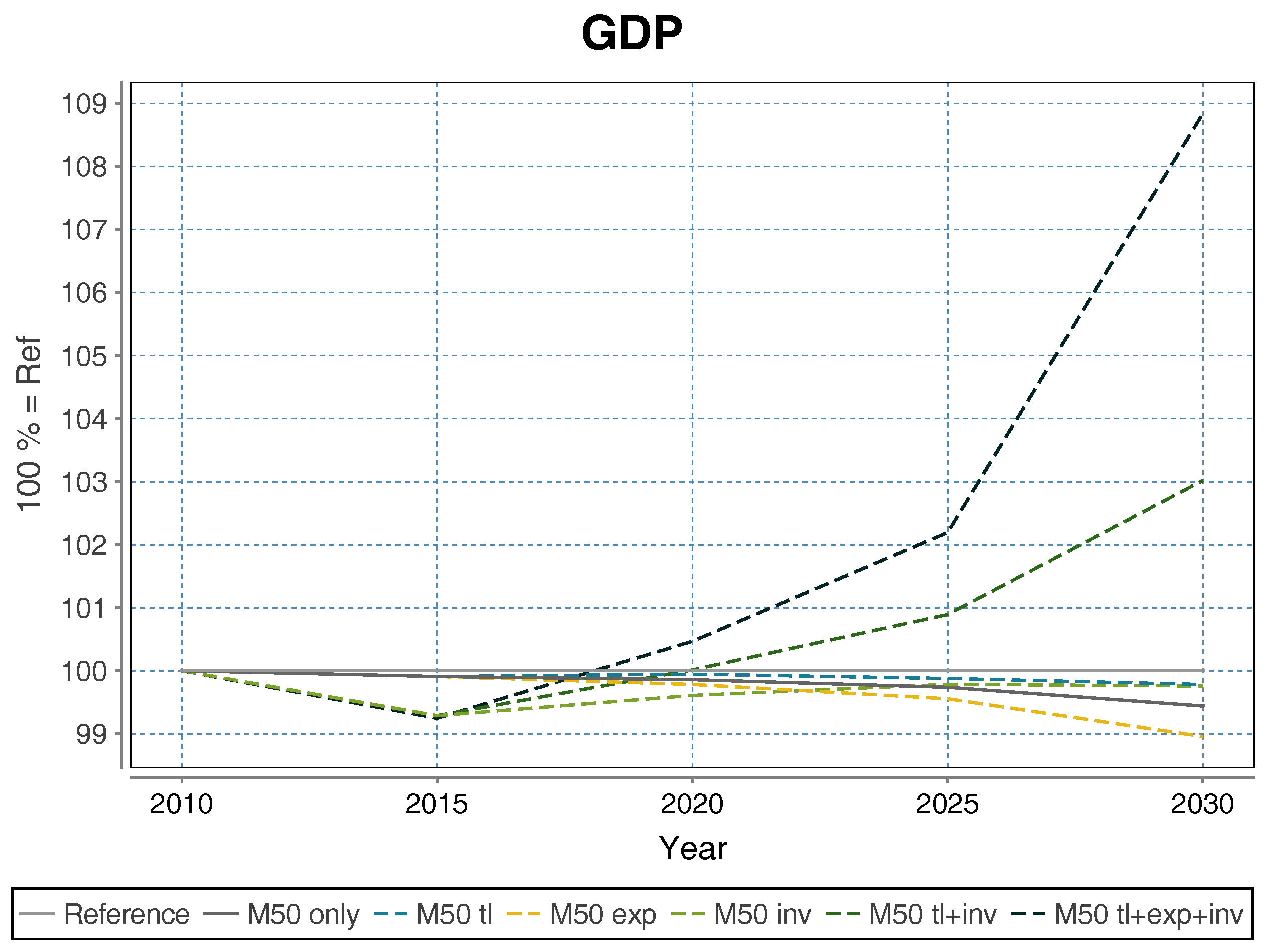
The development over time (see Figure 2) from 2015 to 2030, shows that the investment program causes a reduction of GDP at first. This can be explained by the the first round effect where investment is crowding-out consumption and the fact that positive effects from the additional investment are only realized in the next time step, hence after 5 years.
3.2. Sectoral Impacts
The sectoral disaggregation is what distinguishes CGE models from optimal growth models, which are also used for assessments of economic impacts of climate policy. Results at sectoral level can give us insights into crowding-out of investment between sectors. The sectoral dimension is also important for finding out which sectors will contribute most to the transformation in terms of emission reduction (relevant for climate policy) as well as in terms of economic development (important for economic, labour and education policy).
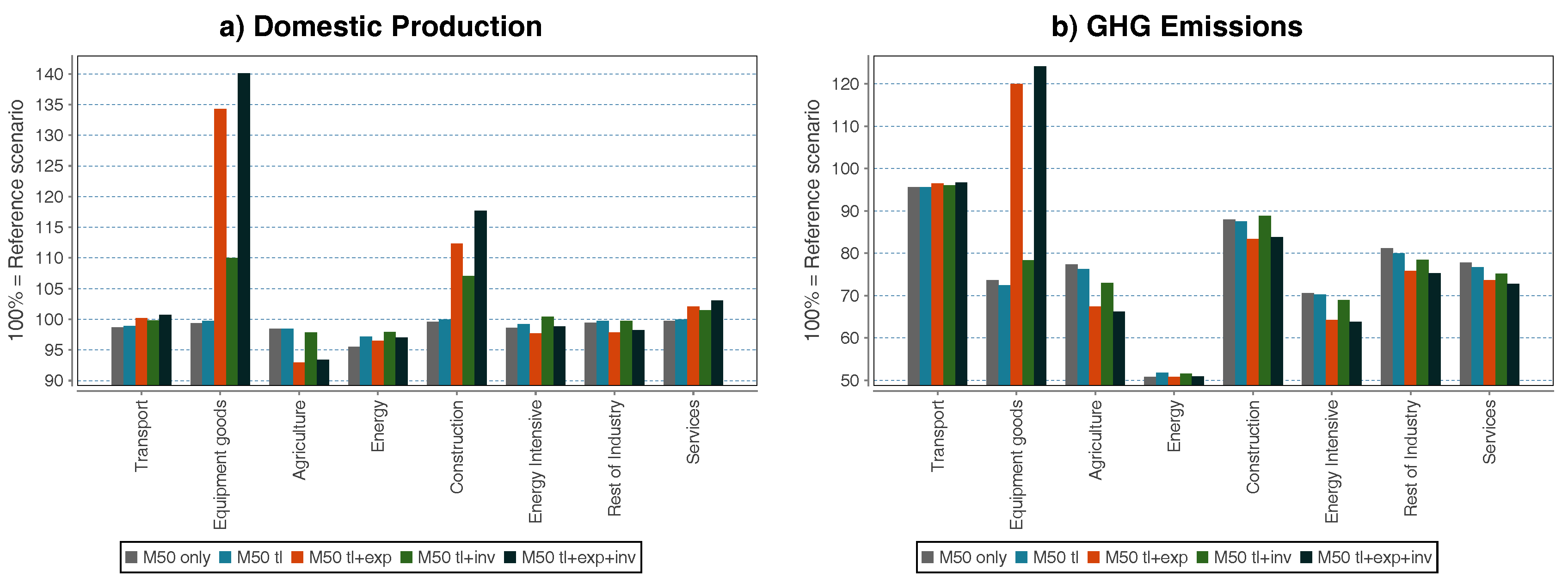
The changes in production levels and emissions of the different sectors are presented in Figure 3. The energy sector shows the largest emission reductions (approximately 50% compared to the reference scenario, for every alternative scenario), hence this is the sector that needs to contribute most to the abatement process. The energy-intensive industry will also reduce emission levels considerably. The transport sector is expected to contribute the least to emission reductions. Equipment goods producers will increase emissions, but much less than the increase of the production level. The overall reduction of GHG emissions is 50% in all scenarios, due to the binding constraint on these emissions.
In economic terms, sectors contributing to energy efficiency improvements, such as construction, equipment goods and services will show higher domestic production due to larger investment in these sectors. Also at sectoral level, we can see a crowding-out effect of the investment program from some sectors to others. This outcome again supports Proposition 3.
4. Discussion
Reaching the Sustainable Development Goals, including climate action and affordable clean energy, requires a fundamental socio-economic transformation accompanied by substantial investment in low-carbon infrastructure. However, there has been little macroeconomic analysis that evaluates the effects of a substantial increase of investment in low-carbon technologies. The usual analyses of climate policy show negative economic effects of emission targets, because they are treated as an additional constraint to the optimization process, e.g., in CGE models and additional feedback effects are not taken into account. However, when evaluating the effects of a large increase of investment for the decarbonization of the economy, assuming no effect on technical progress and investors’ expectations does not give a comprehensive picture. Rather, a sustainability transition should be analysed as a non-marginal change of the economic state, driven by behavioral factors and systemic interactions.
This paper identifies key mechanisms that need to be included in a standard computable general equilibrium model to overcome these limitations. These mechanisms are an investment program, technical progress and adaptive expectations. The results of this work highlight the central role of large additional investment and provide a more comprehensive analysis of the effects of climate policy.
The outcomes of the scenarios with single model changes are in line with what can be expected from the literature on macroeconomic climate policy assessment (see e.g., [25,26,27]) and from the model properties: Technical progress partially offsets the negative economic effect of introducing an ambitious emission constraint. The introduction of adaptive expectations alone, amplifies the negative effect, because it depresses sales expectations of firms. An investment program leads to crowding-out of consumption with investment and therefore to less efficient resource allocation.
The results of the combined scenarios (M50 tl + inv and M50 tl + exp, M50 tl + exp + inv), however, add new insights to the literature on the role of technical progress in climate economic models: Technical progress is necessary for positive economic effects of climate policy, but not sufficient. Combining technical progress with an investment program or adaptive expectations leads to positive economic effects. These findings build on Wing [22], who argued that the endogenization of technical progress gives rise to multiple equilibria. Indeed, the partial endogenization of technical progress introduces the possibility for a different economic growth path. The investment program as well as adaptive expectations introduce the possibility of switching between different economic growth paths.
The results provide suggestions for policy makers aiming for ambitious climate goals. If ambitious climate policy (towards 1.5 °C) should bring about more desirable economic outcomes, it should not be implemented in isolation. Instead, green growth policies should be the core of a wider economic program aimed at increasing investment levels and enhancing technical innovation. Green public procurement and green public investment (as proposed in [8]) will be an important element, as well as implementing credible long-term green growth policies that restore confidence and leverage additional private investment [41].
We can draw conclusions on the mechanisms that lead to a change in the direction of the economic effects of climate policy. However, drawing conclusions on the magnitude of the effect requires additional empirical validation and sensitivity analysis. Furthermore, generalizing these results to other countries requires more in depth analysis at the (EU) member state level as well as an extension of the analysis to other countries. Additionally, research on the role of the financial market is required in order to address the question of how to finance such an investment program, how potential funding constraints might reduce the positive effect or whether credit-financed investment can reduce the crowding-out effect.
Acknowledgments
The authors would like to thank Leonidas Paroussos who implemented the model changes in GEM-E3, and provided the model description and simulation results for the different scenarios. Furthermore, the authors thank Rich Rosen and two anonymous reviewers for helpful comments on earlier versions of the paper. The authors gratefully acknowledge financial support by the German Federal Ministry for the Environment, Nature Conservation, Building and Nuclear Safety under Grant 03KSE041 (Bewertungsmodul Klimapolitik) and by the EU projects DOLFINS (Grant 640772) and CoeGSS (Grant 676547). Open access publication was supported by DOLFINS.
Author Contributions
This paper is based on the report “Investment-oriented climate policy: An opportunity for Europe” [6] prepared for the German Federal Ministry for the Environment, Nature Conservation, Building and Nuclear Safety. Carlo C. Jaeger initiated the idea for the approach. All authors contributed to the framing of the research question and specified the changes in the GEM-E3 model. Steffen Fürst analysed and visualized the data. Franziska Schütze conceptualized and wrote the paper with contributions from all other authors.
Conflicts of Interest
The authors declare no conflict of interest.
Appendix A. Short Technical Description of the GEM-E3-M50 Model
This section provides a short technical overview of the GEM-E3-M50 model, as presented in Jaeger et al. [6]. It provides the general structure of the model in order to better understand the model changes described in the paper. This description is based on the detailed model description of GEM-E3, which can be found in the GEM-E3 reference manual [12] and the GEM-E3 model documentation [34].
Appendix A.1. Firms
Firms maximise their profits, subject to technology constraints:
A Constant Elasticity of Substitution (CES) is used as production function. Firms production is modelled via nested production functions so as to explicitly reflect different substitution elasticities among different inputs:
where Q: total output, : Total Factor Productivity, : Capital–Labour–Energy bundle, : Material bundle, : distributional parameters between and , r, and : elasticity of substitution parameters, : Capital–Labour bundle, : Energy bundle, : distributional parameter between and , : intermediate inputs, : distributional parameter among intermediate inputs.
Appendix A.2. Households
Households maximise their utility, subject to an income constraint:
where U: Utility represented by a Linear Expenditure System function, C: Consumption, : Leisure. Households follow a two step decision process. At first they allocate their resources among consumption/labour supply and savings and then they allocate aggregate consumption over different consumption purposes.
where : subsistence minima, : consumption share parameter
Appendix A.3. Government Consumption
Government consumption (GC) is set exogenously (gcexo), GC = gcexo.
Appendix A.4. Investment
The model is recursive dynamic over time, meaning that multiple (static) equilibria are linked over time with a stock-flow-relationship of capital and investment. Agents have myopic expectations with respect to prices, meaning that the set of decision parameters is constant over time. Endogenously specified investment is determined using Tobins’Q (i.e., by comparing the market price of capital with its replacement cost). The motion equation of the capital stock is:
Firms in the current year decide on their optimal capital stock by comparing the rate of return on capital to its replacement cost.
where is a calibrated scale parameter; K is the optimal demand for capital; is the unit cost of investment; d is the depreciation rate; r is the national interest rate and is the (exogenous) expectation on sectoral growth.
Appendix A.5. Labour Supply
The model does not assume full employment of labour. It incorporates the following labour supply curve that inversely relates wages[w] with unemployment rate [unrt]:
Appendix A.6. GHG Emissions
Energy related CO emissions are calculated by applying the appropriate emission factors to fossil fuel burning.
Process related GHG emissions are linked with the volume of production
The imposition of a GHG emission reduction target generates a dual value that increases the user cost of the emitting activity.
Appendix B. Reference Scenario
Table A1 shows annual growth rates and Table A2 the labour market outcomes from 2015 to 2030 for the reference scenario.

Table A1.
Macroeconomic annual growth rates of the Reference Scenario.
| EU-28 | 2015–2020 | 2020–2025 | 2025–2030 |
|---|---|---|---|
| Gross Domestic Product | 1.5% | 1.6% | 1.5% |
| Investment | 1.4% | 1.6% | 1.5% |
| Public Consumption | 1.6% | 1.6% | 1.5% |
| Private Consumption | 1.6% | 1.7% | 1.6% |
| Exports | 2.0% | 2.0% | 2.1% |
| Imports | 2.3% | 2.3% | 2.3% |
| Labour productivity | 1.2% | 1.6% | 1.7% |
Table A2.
Labour Market Outcomes of the Reference Scenario.
| EU-28 | 2015 | 2020 | 2025 | 2030 |
|---|---|---|---|---|
| Employment (in m. persons) | 224 | 227 | 227 | 225 |
| Population (in m. persons) | 434 | 436 | 432 | 425 |
| Labour Force (in m. persons) | 101 | 102 | 101 | 99 |
| Unemployment rate | 11% | 10% | 9% | 9% |
References
- Wolf, S.; Schütze, F.; Jaeger, C.C. Balance or Synergies between Environment and Economy—A Note on Model Structures. Sustainability 2016, 8, 761. [Google Scholar] [CrossRef]
- Antal, M.; van den Bergh, J.C.J.M. Green growth and climate change: Conceptual and empirical considerations. Clim. Policy 2016, 16, 165–177. [Google Scholar] [CrossRef]
- Jaenicke, M. “Green Growth”: From a growing eco-industry to economic sustainability. Energy Policy 2012, 48, 13–21. [Google Scholar] [CrossRef]
- Pollin, R. Greening the Global Economy; MIT Press: Cambridge, MA, USA, 2015. [Google Scholar]
- Jaeger, C.C.; Paroussos, L.; Mangalagiu, D.; Kupers, R.; Mandel, A.; Tábara, J.D. A New Growth Path for Europe: Generating Prosperity and Jobs in the Low-Carbon Economy; Synthesis Report; A Study Commissioned by the German Federal Ministry for the Environment; Nature Conservation and Nuclear Safety: Berlin, Germany, 2011. [Google Scholar]
- Jaeger, C.C.; Schütze, F.; Fürst, S.; Mangalagiu, D.; Meißner, F.; Mielke, J.; Steudle, G.A.; Wolf, S. Investment-Oriented Climate Policy: An opportunity for Europe; A Study Commissioned by the German Federal Ministry for the Environment; Nature Conservation, Building and Nuclear Safety: Berlin, Germany, 2015. [Google Scholar]
- Guo, L.L.; Qu, Z.; Tseng, M.L. The interaction effects of environmental regulation and technological innovation on regional green growth performance. J. Clean. Prod. 2017, 162, 864–902. [Google Scholar] [CrossRef]
- UNEP. Towards a Green Economy: Pathways to Sustainable Development and Poverty Eradication; United Nations Environment Programme: Nairobi, Kenya, 2011. [Google Scholar]
- World Economic Forum. The Green Investment Report. The Ways and Means to Unlock Private Finance for Green Growth. A Report of the Green Growth Action Alliance; World Economic Forum: Colony, Switzerland, 2013. [Google Scholar]
- Global Commission on the Economy and Climate. Better Growth, Better Climate. The New Climate Economy Report. In The Global Report; The New Climate Economy/World Resources Institute: Washington, DC, USA, 2014. [Google Scholar]
- OECD. Investing in Climate, Investing in Growth; OECD Publishing: Paris, France, 2017. [Google Scholar]
- Capros, P.; Georgakopoulos, T.; Filippoupolitis, A.; Kotsomiti, S.; Atsavesand, G.; Proost, S.; van Regemorter, D.; Conrad, K.; Schmidt, T. The GEM-E3 Model: Reference Manual; National University of Athens: Athens, Greece, 1999. [Google Scholar]
- Van der Ploeg, R.; Withagen, C. Green Growth, Green Paradox and the global economic crisis. Environ. Innov. Soc. Trans. 2013, 6, 116–119. [Google Scholar] [CrossRef]
- Intergovernmental Panel on Climate Change. Climate Change 2014: Mitigation of Climate Change; Contribution of Working Group III to the Fifth Assessment Report of the Intergovernmental Panel on Climate Change; IPCC Working Group III Contribution to AR5; Cambridge University Press: Cambridge, UK, 2014; Volume 1, pp. 1–1455. [Google Scholar]
- OECD. Climate Change: Meeting the Challenge to 2050; Policy Brief; OECD: Paris, France, 2008; pp. 1–8. [Google Scholar]
- Kriegler, E.; Tavoni, M.; Aboumahboub, T.; Luderer, G.; Calvin, K.; Demaere, G.; Krey, V.; Riahi, K.; Rösler, H.; Schaeffer, M.; et al. What Does The 2 °C Target Imply For A Global Climate Agreement In 2020? The Limits Study On Durban Platform Scenarios. Clim. Chang. Econ. (CCE) 2013, 4, 1340008. [Google Scholar] [CrossRef]
- European Commission Staff. Accompanying the Communication: A Policy Framework for Climate and Energy in the Period from 2020 up to 2030; Commission Staff Working Paper; European Commission Staff: Brussels, Belgium, 2014. [Google Scholar]
- Rosen, R.A. Is the IPCC’s 5th Assessment a denier of possible macroeconomic benefits from mitigating climate change? Clim. Chang. Econ. 2016, 7, 1640003. [Google Scholar] [CrossRef]
- Rosen, R.A.; Guenther, E. The Energy Policy Relevance of the 2014 IPCC Working Group III Report on the Macro-Economics of Mitigating Climate Change. Energy Policy 2016, 93, 330–334. [Google Scholar] [CrossRef]
- Stern, N. The Economics of Climate Change. The Stern Review; Cambridge University Press: Cambridge, UK, 2007. [Google Scholar]
- IEA. World Energy Investment Outlook; International Energy Agency: Paris, France, 2014. [Google Scholar]
- Wing, I.S. Representing induced technological change in models for climate policy analysis. Energy Econ. 2006, 28, 539–562. [Google Scholar] [CrossRef]
- Hicks, J. The Theory of Wages; Macmillan: London, UK, 1932. [Google Scholar]
- Acemoğlu, D.; Aghion, P.; Bursztyn, L.; Hemous, D. The Environment and Directed Technical Change. Am. Econ. Rev. 2012, 102, 131–166. [Google Scholar] [CrossRef] [PubMed]
- Popp, D. ENTICE: Endogenous technological change in the DICE model of global warming. J. Environ. Econ. Manag. 2004, 48, 742–768. [Google Scholar] [CrossRef]
- Grübler, A.; Messner, S. Technological change and the timing of mitigation measures. Energy Econ. 1998, 20, 495–512. [Google Scholar] [CrossRef]
- Grubb, M.; Chapuis, T.; Duong, M.H. The economics of changing course: Implications of adaptability and inertia for optimal climate policy. Energy Policy 1995, 23, 417–431. [Google Scholar] [CrossRef] [Green Version]
- Bryant, J. A Simple Rational Expectations Keynes-Type Model. Q. J. Econ. 1983, 98, 525–528. [Google Scholar] [CrossRef]
- Cooper, R.; John, A. Coordinating Coordination Failures in Keynesian Models. Q. J. Econ. 1988, 103, 441–463. [Google Scholar] [CrossRef]
- Arrow, K.J.; Debreu, G. Existence of an Equilibrium for a Competitive Economy. Econ. Soc. 1954, 22, 265–290. [Google Scholar] [CrossRef]
- Boeters, S.; Savard, L. The Labour Market in CGE Models; ZEW—Centre for European Economic Research: Mannheim Germany, 2011; pp. 1–95. [Google Scholar]
- Balistreri, E.J.; Rutherford, T.F. Chapter 23—Computing General Equilibrium Theories of Monopolistic Competition and Heterogeneous Firms. In Handbook of Computable General Equilibrium Modeling; Dixon, P.B., Jorgenson, D.W., Eds.; Elsevier: Amsterdam, The Netherlands, 2013; Volume 1, pp. 1513–1570. [Google Scholar]
- Tarr, D.G. Chapter 6—Putting Services and Foreign Direct Investment with Endogenous Productivity Effects in Computable General Equilibrium Models. In Handbook of Computable General Equilibrium Modeling; Dixon, P.B., Jorgenson, D.W., Eds.; Elsevier: Amsterdam, The Netherlands, 2013; Volume 1, pp. 303–377. [Google Scholar]
- Capros, P.; van Regemorter, D.; Paroussos, L.; Karkatsoulis, P.; Fragkiadakis, C.; Tsani, S.; Charalampidis, I.; Revesz, T. GEM-E3 model documentation. JRC Sci. Policy Rep. 2013, 26034. [Google Scholar] [CrossRef]
- Tobin, J. A general equilibrium approach to monetary theory. J. Money Credit Bank. 1969, 1, 15–29. [Google Scholar] [CrossRef]
- Bowen, A.; Fankhauser, S.; Stern, N.; Zenghelis, D. An Outline of the Case for a ’Green’ Stimulus; Policy Brief; Grantham Research Institute on Climate Change and the Environment: London, UK; Centre for Climate Change Economics and Policy: Leeds, UK, 2009. [Google Scholar]
- Edenhofer, O.; Stern, N. Towards a global green recovery. Recommendations for immediate G20 action. In Report Submitted to the G20 London Summit; Potsdam Institute for Climate Impact Research: Potsdam, Germany; Grantham Research Institute on Climate Change and the Environment: London, UK, 2009. [Google Scholar]
- Zenghelis, D. A Macroeconomic Plan for a Green Recovery; Grantham Research Institute on Climate Change and the Environment: London, UK; Centre for Climate Change Economics Policy Paper: Leeds, UK, 2011. [Google Scholar]
- Beyerle, H.; Fricke, T. A Climate Deal to Rescue Europe. In Proceedings of the Workshop Report: A European Climate Foundation Workshop, Berlin, Germany, 7–8 May 2014. [Google Scholar]
- Schepelmann, P.; Stock, M.; Koska, T.; Schüle, R.; Reutter, O. A Green New Deal for Europe: Towards Green Modernisation in the Face of Crisis; Green New Deal Series; Green European Foundation: Luxembourg, 2009; Volume 1. [Google Scholar]
- Zenghelis, D. A Strategy for Restoring Confidence and Economic Growth through Green Investment and Innovation; Grantham Research Institute on Climate Change and the Environment: London, UK; Centre for Climate Change Economics and Policy: Leeds, UK, 2012. [Google Scholar]
- Romani, M.; Stern, N.; Zenghelis, D. The basic economics of low-carbon growth in the UK. In Policy Brief; Grantham Research Institute on Climate Change and the Environment: London, UK; Centre for Climate Change Economics and Policy: Leeds, UK, 2011. [Google Scholar]
- Arrow, K.J. The Economic Implications of Learning by Doing. Rev. Econ. Stud. 1962, 29, 155–173. [Google Scholar] [CrossRef]
- Wright, T. Factors affecting the cost of airframes. J. Aeronaut. Sci. 1936, 3, 112–118. [Google Scholar] [CrossRef]
- Nagy, B.; Farmer, J.D.; Trancik, J.E.; Bui, Q.M. Testing Laws of Technological Progress; SFI Working Paper; Santa Fe Institute: Santa Fe, NM, USA, 2010. [Google Scholar]
- European Commission. The 2012 Ageing Report. Economic and Budgetary Projections for the 27 EU Member States (2010–2060); European Commission: Brussels, Belgium, 2012. [Google Scholar]
Figure 1.
Results for GDP and employment, energy consumption and energy intensity in 2030, comparing all counterfactual scenarios with the reference scenario.
Figure 1.
Results for GDP and employment, energy consumption and energy intensity in 2030, comparing all counterfactual scenarios with the reference scenario.

Figure 2.
Results for GDP over time.

Figure 3.
Results by sector for production levels and GHG emissions compared to the reference scenario in 2030.
Figure 3.
Results by sector for production levels and GHG emissions compared to the reference scenario in 2030.

Table 1.
Scenario description.
| Abbreviation | Scenario | Description |
|---|---|---|
| Ref | Reference | Optimal path, assuming a business-as-usual policy framework |
| M50 only | M50 | 50% reduction of GHG emissions compared to 1990 |
| M50 inv | M50 with investment program | Part of the investment required to decarbonize the EU economy is financed by increasing consumption taxes |
| M50 tl | M50 with technical progress | Learning by doing effects are introduced in the sectors producing both clean energy technologies and other equipment goods |
| M50 exp | M50 with adaptive expectations | The investment decision of firms is adjusted so as incorporate expectation dynamics, next to myopic expectations |
| M50 tl + inv | M50 with technical progress and investment program | |
| M50 tl + exp | M50 with technical progress and adaptive expectations | |
| M50 tl + exp + inv | M50 with technical progress, adaptive expectations and investment program |
Table 2.
Macroeconomic results, all scenarios compared to reference in 2030.
| M50 only | M50 tl | M50 exp | M50 inv | tl + exp + inv | |
|---|---|---|---|---|---|
| GDP | −0.56% | −0.22% | −1.04% | −0.24% | +9.73% |
| Employment | −0.76% | −0.46% | −1.41% | −1.21% | +1.18% |
| Energy Use | −4.91% | −3.83% | −5.57% | −4.87% | −2.73% |
© 2017 by the authors. Licensee MDPI, Basel, Switzerland. This article is an open access article distributed under the terms and conditions of the Creative Commons Attribution (CC BY) license (http://creativecommons.org/licenses/by/4.0/).
Share and Cite
MDPI and ACS Style
Schütze, F.; Fürst, S.; Mielke, J.; Steudle, G.A.; Wolf, S.; Jaeger, C.C. The Role of Sustainable Investment in Climate Policy. Sustainability 2017, 9, 2221. https://doi.org/10.3390/su9122221
AMA Style
Schütze F, Fürst S, Mielke J, Steudle GA, Wolf S, Jaeger CC. The Role of Sustainable Investment in Climate Policy. Sustainability. 2017; 9(12):2221. https://doi.org/10.3390/su9122221
Chicago/Turabian StyleSchütze, Franziska, Steffen Fürst, Jahel Mielke, Gesine A. Steudle, Sarah Wolf, and Carlo C. Jaeger. 2017. "The Role of Sustainable Investment in Climate Policy" Sustainability 9, no. 12: 2221. https://doi.org/10.3390/su9122221
Note that from the first issue of 2016, this journal uses article numbers instead of page numbers. See further details here.