Modeling the Impact of Urban Landscape Change on Urban Wetlands Using Similarity Weighted Instance-Based Machine Learning and Markov Model

1
Department of Social Sciences, College of Liberal & Fine Arts, Tarleton State University, 1333 W Washington St, Stephenville, TX 76402, USA
2
Department of Geosciences, College of Arts & Sciences, University of Missouri-Kansas City, 5100 Rockhill Road, Kansas City, MO 64110, USA
*
Author to whom correspondence should be addressed.
Sustainability 2017, 9(12), 2223; https://doi.org/10.3390/su9122223
Submission received: 28 September 2017
/
Revised: 29 November 2017
/
Accepted: 29 November 2017
/
Published: 1 December 2017
(This article belongs to the Special Issue Wetland Ecology, Conservation and Sustainability: Applications of Geospatial Techniques)
Abstract
:Urban wetlands play important roles in providing several ecosystem services that support the urban environment. As such, scientists have studied them to understand the urban processes that lead to their continued decline. However, little attention has been given to the drivers of land-use change that may affect this fragile ecosystem in the future. Understanding this could serve as a critical step towards urban wetland management and sustainability. In this study, we utilized an integrated approach that combined Similarity Weighted Instance-based Machine Learning and Markov chain, both embedded in the IDRISI Land Change Modeler to simulate change in the landscape of three watersheds in the Kansas City Metropolitan area. The purpose was to assess the possible future impacts of urban expansion-induced landscape change on wetlands within the study area, using a retrospective approach. To achieve this, classified SPOT satellite data covering the three watersheds were used to generate historical land cover maps of the study area between 1992 and 2010 to analyze changes to the landscape. In addition, the study identified several drivers of land change associated with the historical change process in the study area, and accounted for their role in the modeling process. On this basis, the study made the prediction of urban landscape transformation to the end date of 2014. The prediction result was verified with a more accurate map that was derived from independently classifying a 2014 SPOT image of the study area. Results from this study show that impervious surfaces, which were used as an index of urban expansion, may increase by approximately the same magnitude experienced historically, which may result in a small but significant loss of wetlands and other land cover classes within the study area.
1. Introduction
Various stakeholders utilize urban landscapes for multiple purposes such as housing, infrastructures, and services, among others. Several of these uses lead to a permanent transformation of many urban landscapes that result in both negative and positive consequences. While urban development projects that boost the economy of urban centers are viewed as positive outcomes of urbanization, ecologically speaking, urbanization has a negative effect on the natural environment [1]. Urban landscapes have experienced remarkable changes over the years. From purely rural or sometimes uninhabited natural lands, many have transformed to complex urban landscapes. Because of these changes, several studies (e.g., [2,3,4,5,6,7,8,9,10,11]) have examined the changing urban landscapes of several locations globally. For instance, within the United States, researchers have sought to understand the dynamics of urban landscape changes to account for their causes, patterns, responses and implications [12,13]. Jones et al. [12] considered landscape change to be one of the greatest threats to aquatic and terrestrial resources in many areas of the United States, which have had a negative effect on surface waters and terrestrial habitats, especially forests in many parts of the nation. This is the situation for many other areas around the world. Apart from these studies, many attempts have also been made to simulate possible future change in urban landscapes using spatial models (e.g., [13,14,15,16,17]). The purpose of many of these studies is to understand how the urban landscape may develop in the future, so planned outcomes can be incorporated into the developmental process and strategic urban planning. One notable and significant direct result of urban development is the increase in impervious surfaces in urban areas when compared to the suburban areas. Increase in impervious surfaces has been used as an indicator of urban ecosystems degradation [2]. Kauffman and Brant [18] observed a strong relationship between impervious surface increase and decline in stream water quality as well as wildlife habitat loss in the United States. While historical studies of urban landscape change have improved our understanding of previous landscape change dynamics, accurate simulation of future landscape change is still challenging because of error propagation and uncertainty issues with input data of several landscape modeling studies. This is particularly important when consideration is given to the impacts that changed urban landscapes have on wetlands as a complex, dynamic, yet vulnerable and less-studied component of urban ecosystems. Often, these impacts manifest in the degradation or complete loss of urban wetlands caused by urban expansion.
Urban wetlands provide various ecosystem services, including improvement of water quality, floodwater storage, fish and wildlife habitat, aesthetics, and biological productivity [19]. In the United States, wetlands form an integral part of the national heritage [20,21]. Nevertheless, many complex factors have been shown to affect them negatively, such as anthropogenic disturbances that usually alter the landscape and natural ecosystems. Anthropogenic effects are usually more significant in the light of their large-scale effects, which typically takes place through landscape modifications or alterations. As part of urban development, specific human activities like dredging, ditching, filling, draining, and plowing have the most direct and obvious impacts on urban wetlands. Between 2004 and 2009, an estimated 253 km2 of wetlands were lost in the United States [22]; many of them were in urbanized areas. However, many deliberate public and private efforts have sought to mitigate damages to wetlands and protect them through acquisition, restoration, enhancement, and production [22], for which understanding wetland dynamics in relation to the urbanization process is the key.
While many studies have examined the effects of urban developments on urban wetlands in the past (e.g., [2,23]), little is known about how increased development may affect this fragile ecosystem in the future. This is particularly challenging in urban areas because wetlands may be subject to intensified, coupled impacts of human disturbances and precipitation variation in complex urban landscapes [2]. Therefore, the goal of this study is to examine the possible future impacts of urban expansion as a catalyst of urban landscape change on urban wetlands. Emphasis is placed on the impacts of urban expansion on urban wetlands because of their large-scale effects in altering the urban landscape. We utilized impervious surfaces as an index of urban expansion, and we assessed the impacts of increased impervious surfaces on urban wetlands in the study area. Central to this study is the question: What was, and what will be, the dynamic effects of urban expansion on urban wetlands in the study area? Dynamics used in this study include all aspects of wetland loss such as where within the watershed is loss occurring the most?
To achieve the goal of this study, we used the Land Change Modeler for Ecological Sustainability in IDRISI Selva, which integrates Similarity Weighted Instance-based Machine Learning and a Markov model, to simulate the landscape change of three watersheds in the Kansas City area. Based on the simulation results, the study assessed the impacts of future landscape change on urban wetlands. The Similarity Weighted Instance-based Machine Learning, described by Sangermano et al. [24] was used in predicting the potential for the locations being examined to change from one time to another time using known instances of change in the study area. The outputs from this process are maps representing the potential for change in the locations under examination. A Markov chain makes use of these potentials for change from one time to another time to describe the actual change, and then uses this information to project the change to a later time. Many studies have integrated Markov chain with other transition potential modeling methods such as the multi-layer perceptron neural network and cellular automata methods (e.g., [25,26]). This study utilized the Similarity Weighted Instance-based Machine Learning approach in combination with Markov chain because it has the capacity to predict transition potentials without the need for complex parameters [24] associated with other methods. The results obtained from integrating both methods of landscape simulation were used in assessing the impact of urban expansion induced landscape change on wetlands within the study area. While the methodology of urban landscape change modeling that was used in this study is not new, its application for assessing the effects of urban landscape change on urban wetland is still relatively new and less studied.
2. Materials and Methods
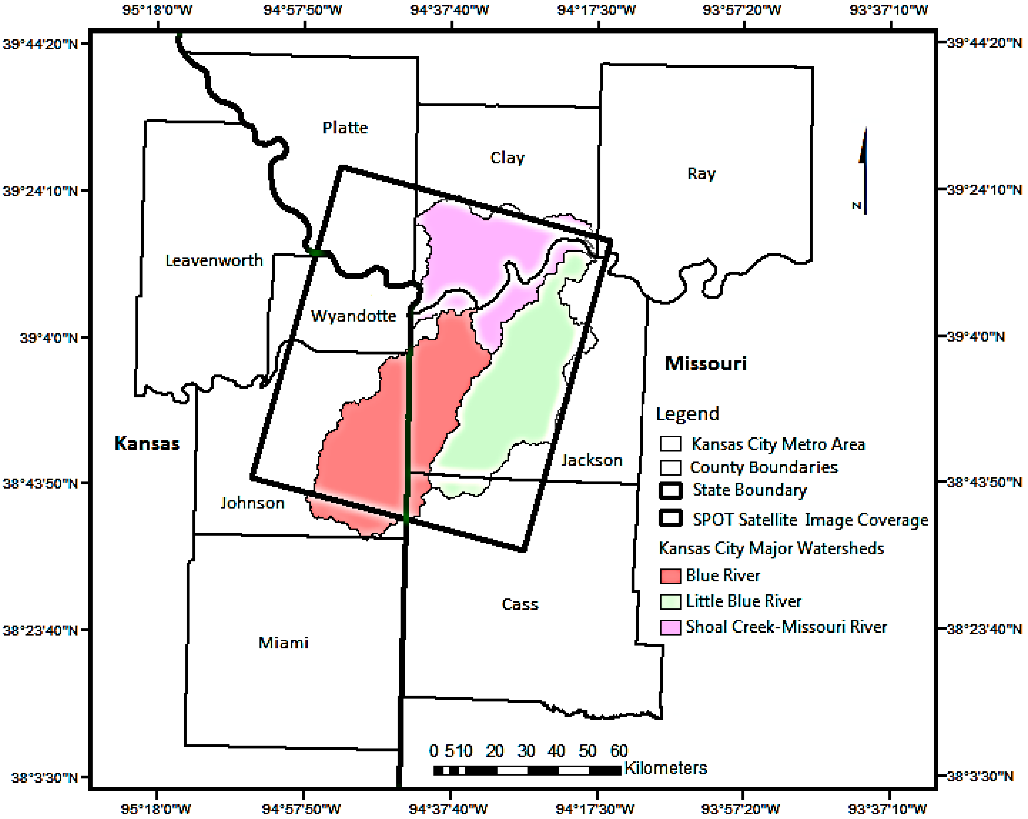
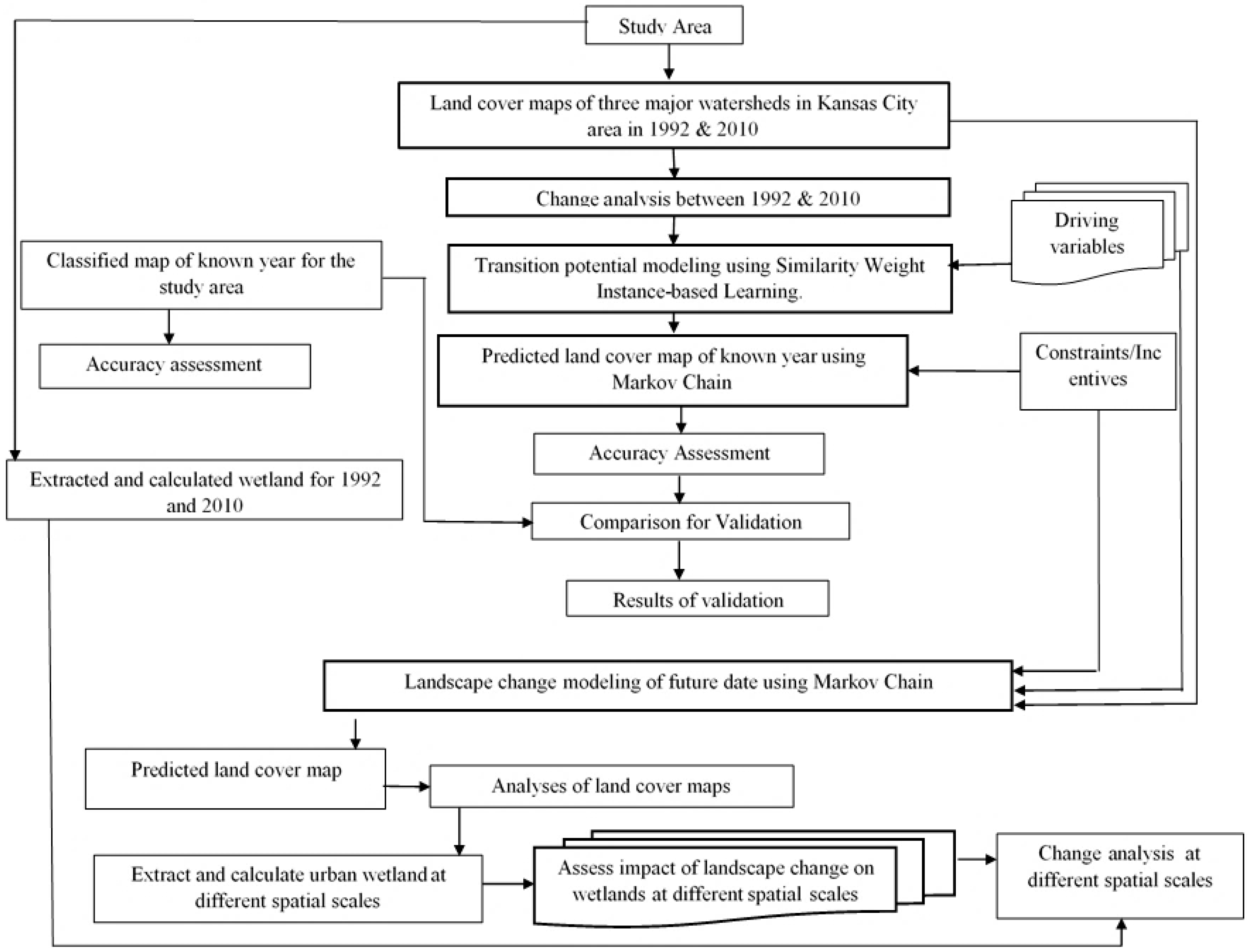
This study includes the classification of two SPOT satellite images, which were used for the change analysis between 1992 and 2010. In addition, the potential for land to change from one land cover type to another was examined with the Similarity Weighted Instance-based Machine Learning, while Markov chain was used in quantifying the demand for land, and in predicting the future quantity of change. Based on results from these processes, an assessment of the modeled landscape change impact on wetlands within the study area was carried out. Figure 1 is the study area and Figure 2 is the flow chart of the major methods used in this study.
2.1. Study Area
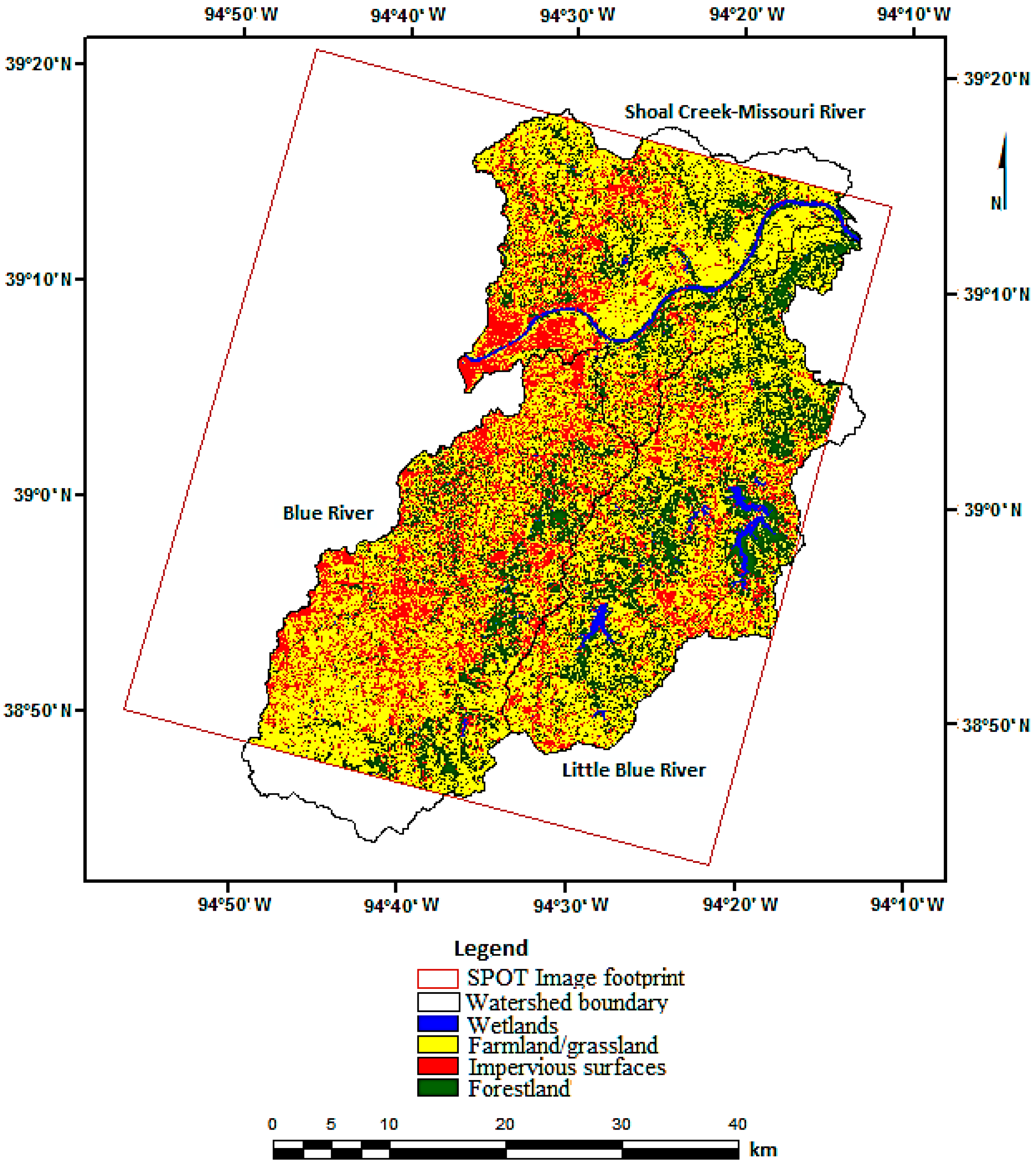
The Kansas City metropolitan is a 14-county metropolitan area that lies within the U.S. states of Missouri and Kansas. It has a total area of about 20,596 km2 and a population of 2,343,008 [27]. With an estimated growth rate of about 11.3% between 2000 and 2010 [27], the area has experienced a remarkable urban expansion. Predominant land cover types of the area are rolling hills and open plains, with grasslands, croplands, forests, urban zones, and scattered water bodies (including open and vegetated wetlands). The area has experienced significant alteration of its natural landscape [28] caused by urban development along with population growth [29]. Of significance is the effect of change on the natural ecosystem such as urban wetlands, which is sensitive to human activities and climate impact. In a recent study, Ji et al. [2] documented the historical impacts of urban expansion on wetlands in the area. Their study showed that smaller wetland areas were more susceptible to human impacts than larger wetland areas. Unfortunately, we do not currently know the effects of these impacts in the future. The study area falls within 9 (Figure 1) out of the 14 counties that make up the metropolitan Kansas City area.
2.2. Datasets
This study used historical SPOT satellite images covering three watersheds (Figure 1 and Table 1) in the Kansas City area in 1992, 2010 and 2014. The goal is to examine the possible future impacts of urban expansion on urban wetlands. These three images were needed to achieve the goal of this study. The process involves beginning (1992) and end images (2010) that determined the time-period for historical change analysis and a third image (2014) that was used for validating the model prediction. Dates of SPOT satellite imageries were chosen based on their availability and accessibility. Hence, there are possibilities of some impacts on the result of this study due to phenological changes, especially because the 1992 SPOT image was acquired in January. However, given the importance of this study, we consider the value of this study to be greater than the potential implications of different phenology in our classification.
The validation map, which was the actual land cover map of 2014, was derived using the maximum likelihood image classification approach. Using high-resolution images from Google Earth, accuracy assessments were conducted on the validation image and the predicted 2014 map. Accuracy assessment results from this process were satisfactory and confirmed the usefulness of both the classified and the predictive maps.
The 1992 image had a spatial resolution of 20 m, while both the 2010 and 2014 images had spatial resolutions of 10 m each (Table 1). To achieve uniformity when comparing the results of prediction, the spatial resolution of the 2010 and 2014 images were resampled from 10 m to 20 m using the nearest neighbor resampling technique. The 1992 and 2010 images were classified by a previous study [2] of urban wetlands dynamics in the study area using an integrated approach that combined knowledge-based and spectral image classification methods. The digital numbers (DN) of the images were used as the basis for classifying these images. Several studies (e.g., [30]) have argued for the conversion of the image DN to surface reflectance before image classification to eliminate the spatially distributed bias that is caused by the none uniform atmospheric effects on the images. However, similar to Song et al., we argue that atmospheric correction is not always necessary for image classification and change detection. Both simple theoretical analysis and empirical results indicate that only when training data from one time or place are applied in another time or place is atmospheric correction necessary for image classification and many change detection methods [30]. Several studies (e.g., [1,2,15,28]) have made use of image DN in classification without the conversion of the DN to surface reflectance. In this study, the training data and spectral signatures used were unique for each image. On this basis, four categories of land cover types were adopted, which can best describe the landscape of the study area on a broad scale: impervious surfaces, farmlands/grasslands, forestlands, and wetlands. Impervious surfaces represent residential areas, shopping centers, industrial and commercial facilities, highways and major streets, and associated properties and parking lots. Forestland cover depicts areas of land with collection of trees. Farmlands/grasslands include areas with grasses, brush, crops and, in general, non-forest vegetation. Grasslands and croplands categories were merged because of the similarity in the spectral signatures of both classes. This was done to avoid the problem of mixed classes between farmlands and grasslands. Wetlands in the study area include open water bodies and vegetated lowlands such as riparian areas. The knowledge-based classification approach used in Ji and coworkers’ study [2] was applied to the wetlands only, because at fine-scales, some wetlands cannot be detected based on their spectral properties using the traditional classification approach [2]. The maximum likelihood classification approach used on the validation image did not pose any problem relating to consistency in methodology because the image was only used for validation purposes. This study furthers Ji and coworkers’ work to examine if previously revealed patterns of landscape change impacts on wetlands will continue into the future in the study area. Google Earth high-resolution images of the three years were used as reference images in conducting accuracy assessments on the classified maps. Accuracy assessment ensures the usefulness and effectiveness of both the classified maps and the predicted map. The stratified random sampling approach described by Jenson [31] was used in selecting 250 points for each image classified and modeled. The results of the accuracy assessments are reported in the results section, including the producer’s and user’s accuracies for each image.
Further, eleven land change driving variables were selected for use in this study (Table 2). Many of these variables have been previously identified as land change variables localized to the study area by the Forecast Technical Committee of the Mid-America Regional Council (MARC) in 2014 while carrying out a forecast of land use change for Kansas City from 2010 to 2040 [32]. Zubair and Ji [1] described and used seven of these variables in a previous study of landscape change modeling in the study area. Land change variables used include the distance from anthropogenic disturbances in 1992, the distance from urbanization and existing infrastructural development, the distance from streams, the land cover likelihood (change likelihood in land cover between 2010 and 2014). The distance from roads, the distance from central business district, the distance from parks and recreation, the distance from park and ride, National Elevation Dataset (NED) of the study area, the slope, and population data of 2010 by blocks are also included. The data layers of these variables were processed to have a spatial resolution of 20 m, so that they can align with the resolutions of the SPOT images. These variables were derived from existing datasets (Table 2 and Table 3). These datasets include the National Elevation Dataset (NED) of the Kansas City area used for both elevation and generating the slope values. Streams data for the study area were used in generating the distance measure from the streams variable, while roads data (interstate highways, state highways, US highways, and marginal/service roads) were used in generating the distance measure from the roads variable. The evidence likelihood, the distance from urban, and the distance from anthropogenic disturbances were extracted from the classified land cover maps of 1992 and 2010. Other datasets used include the study area’s central business district, parks and recreation areas, park and ride locations (locations in the study area where motorists can park and connect to transit or carpool), and 2010 population by blocks. In addition to these, the tax-break development areas were introduced at the model implementation stage. These areas represent distressed communities that have received tax breaks as development incentives to encourage development within the study area. In addition, development constraints in form of public land ownership, nationally conserved lands, and privately protected areas that were provided voluntarily were introduced at this stage. Transitions were reduced within the development constraint areas to reduce the chances of development during the model implementation stage.
2.3. Procedures for Deriving the Landscape Change Driving Variables
The land change driving variables in the dataset section were derived using the following procedures:
Land cover likelihood: This is an empirical likelihood of change between an early land cover image and a later image. In this case, we examined the likelihood that the different land cover categories will change between 2010 and 2014. The results revealed the likelihood of finding the land cover class at the pixels being examined if these pixels represent an area that would change.
Distance from anthropogenic disturbances: To obtain this, we assumed that new areas of disturbances in 2010 would have proximity to areas of existing disturbances in 1992. This is because economic costs of providing new infrastructure are usually considered before developing new lands. Therefore, all previously disturbed areas in 1992 were extracted from the 1992 classified map. These disturbed areas are the areas that were once forest but have been converted to impervious surfaces and farmlands. A distance calculation was run on the results to produce the distance from anthropogenic disturbances variable. This distance is a Euclidean distance between each pixel and the closest set of target features, which in this case are the anthropogenic disturbances.
Other variables include the distance from streams, the distance from roads, the distance from urban area, the elevation, the slope variable, the distance from central business districts, the population data of 2010 by block, the distance from park and ride and the distance from parks and recreation. The IDRISI software has the distance module that was used in generating all the distance variables used in this study.
2.4. Procedures for Processing the Constraints and Incentives Datasets
2.4.1. Constraints
The constraints used are nationally conserved lands and privately protected areas. This dataset was obtained from the Protected Area Database (PAD) of the United States. One layer with sixteen polygons of various sizes represented the protected areas on the map. This dataset was rasterized. The values of the rasterized map ranged from 0.0 to 16.0. These numbers are IDs assigned by the software to the protected and unprotected areas of the input data in the rasterization process. Values 1.0–16.0 are counts of the polygons that represented the protected areas, while “0.0” represented areas unprotected (no polygons). Each polygon was then assigned an ID in the process of rasterization based on the polygon counts. To use these data, the rasterized map was reclassified to assign the value of “0.0” to protected areas since development is not allowed in these areas, and a value of “1.0” to unprotected areas, where development is allowed.
2.4.2. Incentives
These incentives are polygons of distressed municipalities and communities that have been given tax-credit as incentives for development. The incentive areas were applied in the model implementation stage. Although the dataset was for 2009 (Table 3), it was assumed that the areas had the same conditions that accorded them the tax-credit status in 2009 prior to 2009. Further, incentives were not usually for one year, but for longer periods until significant progress was made in development. The incentives dataset was rasterized. The result of this operation produced the incentives map ranging from 0.0 to 181.0 values. These values were associated with the map area, i.e., locations within the study area where no incentives exist and polygons within the map area that represented municipalities and communities that benefited from incentives. These values were reclassified for ease of use. Areas without incentives—meaning that the vulnerability to change will remain the based modeled vulnerability—had 1.0 value. Values above 1.0 are incentives, i.e. vulnerability increases, while values below 1.0 and just greater than 0.0 are disincentives, meaning that the vulnerability will decrease.
To apply both the constraints and the incentives together in the model implementation stage, the two datasets must be combined as one layer. To do this, both the incentives map and the constraint map were overlaid to produce a single layer. This yielded an incentive/constraint map with values ranging from 0.5 to 2.5, where 0.5 represented constraints, while 2.5 represented incentives. The range between these two values represents “no incentives” and “no constraints” (i.e., areas on the map where neither constraints nor incentives were present). For ease of processing, the constraints data were reclassified from 0.5 to 0.0 and the incentives from 2.5 to 1.1. The resulting map (the incentives and constraints map) is then multiplied with the probability of change associated with each transition during the change prediction process.
2.5. Procedures for Simulating Landscape Change of the Three Watersheds under Study
A knowledge-based classification approach from a previous study [2] was used in classifying all the input images (1992 and 2010) used in the study area (Figure 4 and Table 4). The 2014 image that was used for validating the predicted map was additionally classified for this research using the widely used supervised maximum likelihood classification approach (e.g., [33]). Details of the landscape simulation procedure are shown below.
2.5.1. Historical Change Analysis
Once the images and their accuracy assessments were obtained, the change in land cover state between the earlier stage (1992) and the later stage (2010) were assessed to identify and quantify past land cover change within the three watersheds. The result was a change map between these two periods. This was the first step to modeling the future state of the landscape.
2.5.2. Modeling the Potential for Change
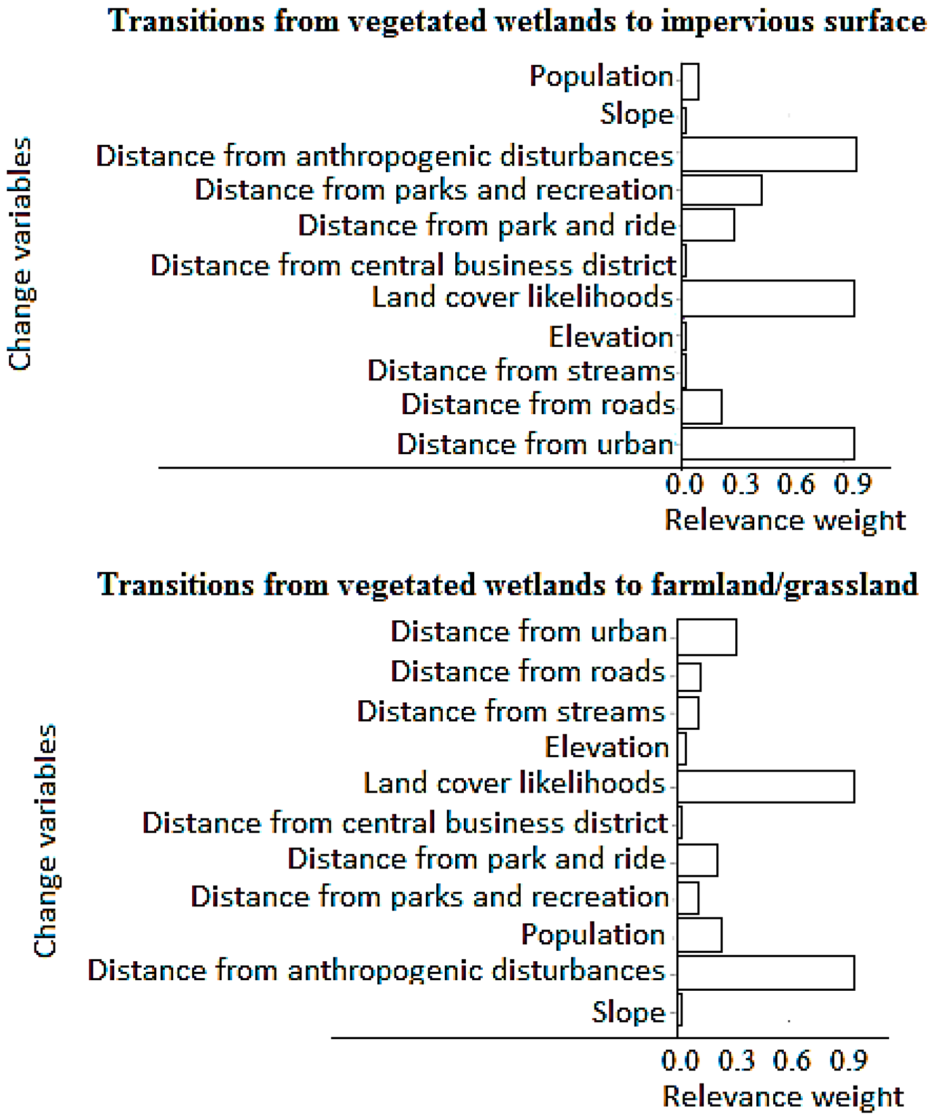
The next step was to model the potential for change to occur on the landscape. This process was based on the results of the historical change analysis conducted for the three study watersheds between 1992 and 2010. The change potential modeling involved modeling the preparedness of the land to change from one state to another. This potential was modeled using a non-parametric method that is integrated with the TerraSet Geospatial Monitoring and Modeling System’s Land Change Modeler (LCM), Similarity Weighted Instance-based Machine Learning (SimWeight). The TerraSet Geospatial Monitoring and Modeling System’s Land Change Modeler (LCM) is an innovative land planning and decision support software tool that simplifies the complexities of land change analysis and prediction [34]. The SimWeight model, well described in Sangermano et al. [24], is an instance-based machine-learning algorithm that is based on a modified K-nearest neighbor machine learning algorithm, which calculates the weighted distance in variable space to known events for the classes. The method identifies the relevance of each land change-driving variable in the change process and predicts the transition potential of locations given known instances of change [24]. Relevance is achieved by variable weighting. Variable weighting is calculated by multiplying each variable by a weight that is proportional to its ability to distinguish between classes [35]. Each variable weight is then determined by comparing the standard deviation of the variable inside areas that have changed to the standard deviation of the variable for the entire study area [24]. A smaller standard deviation of the variable inside the pixels that have changed when compared to the study area as a whole signifies that the variable is relevant for discriminating change [24]. Figure 8 is the relevance weight of each variable that is associated with the six transitions determined for the three watersheds. Transition maps were generated from these six transitions. To generate suitable transition maps, SimWeight identifies “change” and “persistence” for each of the transitions [36]. The K-nearest neighbors of either change or persistence is extracted, and distance is computed in the variable space from each unidentified location to the events of change that occurred in the range of K [36]. Generally, it is recommended to work with a K value of 1/10th of the sample size. Although Eastman et al. [37] reported that the multi-layer perceptron (MLP) neural network performed best when compared with other potential modeling methods [37], Sangermano et al. [24] reported that SimWeight produced similar results with MLP. However, SimWeight is a simpler method that requires less parameterization, hence its use in this study.
The SimWeight approach was used in modeling six transitions using the eleven land change driving variables shown to have association with the historical change process between 1992 and 2010 in the study area. These transitions included transitions from farmland to impervious surface, forestland to impervious surface, forestland to farmland/grassland, vegetated wetlands to impervious surface, farmland/grassland to forestland and open wetlands to vegetated wetlands. Each transition between 1992 and 2010 was used as the basis for modeling the future landscape of the study area. Table 5 showed the result of the goodness of fit of the model.
2.5.3. Integration with Markov Chain for Change Prediction
Based on the historical land change between 1992 and 2010, and the six transition potentials that were modeled using the SimWeight model, we made prediction of urban landscape transformation to an end date of 2014. Markov chain was used in modeling the demand for land between 2010 and 2014. It determined how much change took place between 2010 and 2014. Many studies (e.g., [15,25,38]) have demonstrated the usefulness of Markov chain for landscape simulation. A Markov chain is a stochastic process model that predicts the likelihood of change from one state to another state [39]. The modeling is defined as a set of states where a process begins in one of the states and moves consecutively from one state to another; each move is defined as a step [40]. It makes use of the potential for change in landscape from one time to another time to depict change, and then makes use of this potential to project change to a later time.
The LCM model in IDRISI gave two outputs: soft prediction and hard prediction. The soft prediction represented the vulnerability of the land to experience change [41]. The areas mapped are locations that have not changed but have the ideal condition for change, and may transition at some point [37]. However, the emphasis in this study was limited only to the hard prediction as it was not possible to verify the result of the soft prediction because the result were predictions of the pixels that were likely to change, not the pixels that actually changed. The hard prediction procedure is based on a multi-objective land allocation (MOLA) algorithm [42] that looks through the transitions to identify classes with high potential to lose land and those with high potential to gain land. It then assigns land to the class with the high potential to gain land. The result is a single map of the future state of the landscape in question, which is a scenario of change [37]. During the prediction stage, tax incentives for development and the constraints were introduced. The constraints were used to mark out areas with protected forests where transitions were reduced to minimize the chances of development.
The prediction was first made into 2014 so that the model could be calibrated and validated with the actual land cover map that was derived from independently classifying a 2014 SPOT image of the study area. We validated the predicted map of 2014 using the error matrix approach. We then compared the result of the predicted map of 2014 to that of the actual map classified from the 2014 SPOT image, which served as a reference map. The error matrix is derived from a comparison of reference map pixels with the predicted map pixels. This matrix takes the form of the columns representing the reference data by category and rows representing the predicted map by category [43]. From the error matrix, several measures of prediction accuracy can be calculated. The purpose was to assess the percentage of pixels correctly and incorrectly predicted and to obtain errors of omission, and errors of commission (Table 6).
Based on satisfactory results obtained from validating the 2014 prediction, the model was used in simulating the landscape of three major watersheds in the study area into 2028 using 2010 land cover map as the beginning year image. The study used the historical change period (1992 and 2010) on which future prediction was made as the basis for selecting this end date. This historical period covers 18 years. As such, additional 18 years were added to 2010, resulting in 2028 end date.
2.5.4. Effects of Change on Wetlands
The effects of the modeled landscape by 2028 were assessed on wetlands within the three study watersheds. The wetlands used in this research denoted the combination of surface water bodies and vegetated wetlands that can be detected by optical remote sensing. It also included an assessment of past change between 1992 and 2010 to reveal the historical and temporal dimensions of landscape change effects on wetlands within the study area.
Further, change detection analysis was carried out to examine the pixels that have changed from wetlands to impervious surfaces between 1992 and 2010 and between 2010 and 2028. This was to determine how much urban expansion had affected wetlands in the study area, and how much of such change is expected to happen in the future.
Finally, historical and future precipitation patterns and population projections were examined to see if these factors would influence wetlands in the future.
3. Results
This section presents analysis results of assessing the impact of landscape change on wetlands within three major watersheds in the Kansas City area. First, we examined how errors from mixed classification might affect the accuracy of our classified maps. Figure 3 reveal the difficulty of separating the pixels that represented our classes of interest on all three images. Except for the 1992 image, pixels between the wavelength intervals 0.50 and 1.0 micron on the 2010 image and between 0.50 and 0.70 microns on the 2014 image were difficult to separate into the different classes. However, with careful selection of training sites, this potential error in our classified map was minimized.
3.1. Historical Change Analysis between 1992 and 2010 in the Study Area
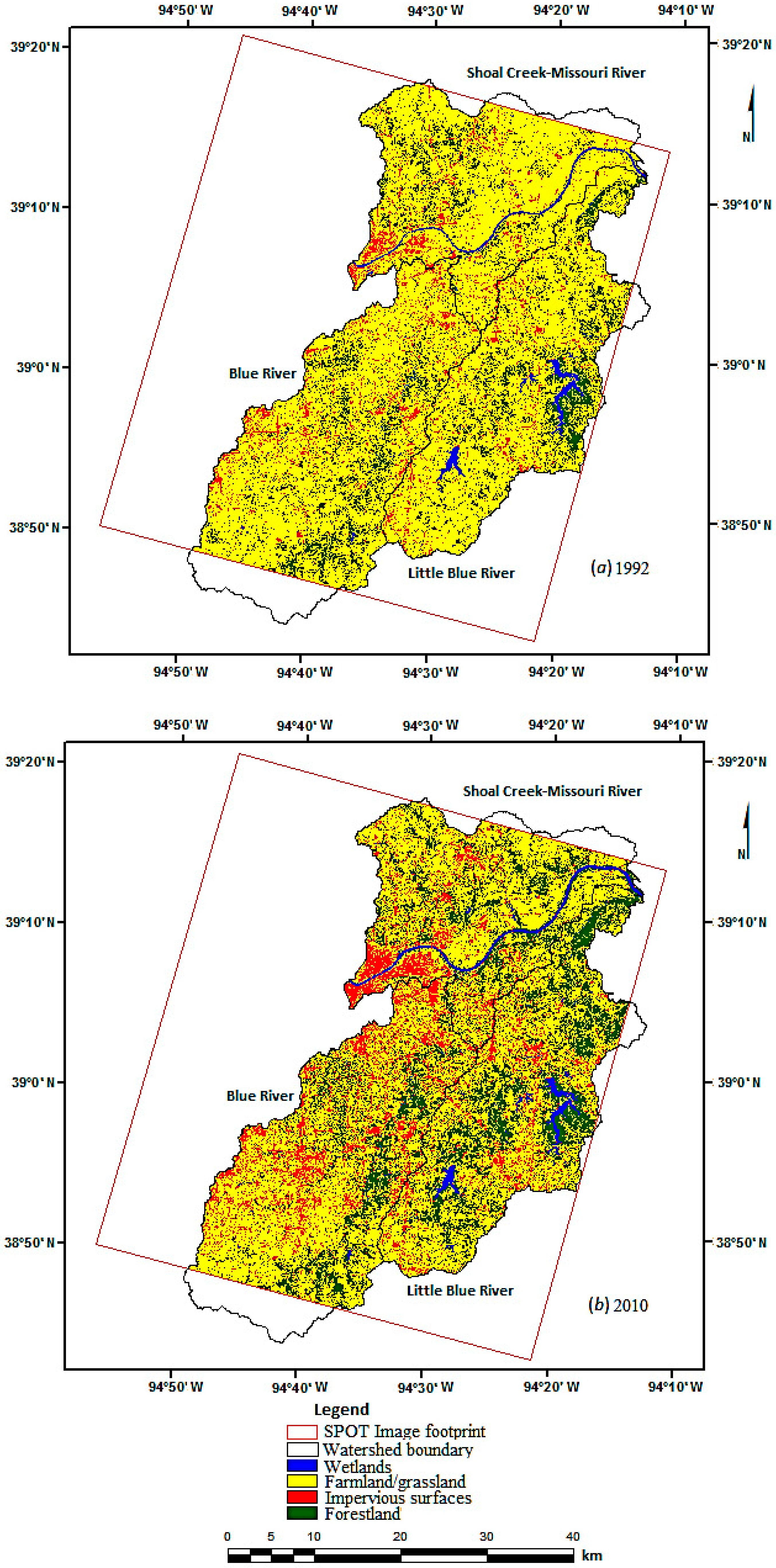
Figure 4 showed the 1992 and 2010 land cover maps, while Table 4 showed their accuracy assessment. Using the 1992 and 2010 land cover maps, a change analysis was conducted between both years. The result reveals increase and decrease in the different land cover types within the watersheds under consideration (Figure 5), including the dynamics of change in wetlands. This study examined open and vegetated wetlands separately, but combined both in the final maps. Both wetlands function differently within the landscape and provide different ecological services. Although both wetlands were combined in the final map, Figure 5 showed that open wetlands increased more, while vegetated wetlands decreased. However, because the increased in open wetlands was more than the decrease in vegetated wetlands, we observe a net increase (Figure 6) of 0.1% (1.4 km2) in wetlands between 1992 and 2010. While this increase is small, we consider this a positive development that should be sustained and improved on. Dynamics of this increase and decrease remains to be examined.
Farmlands/grasslands experienced the largest loss between 1992 and 2010, followed by forestland, and then impervious surfaces (Figure 5). This reveals the degree of susceptibility of both farmlands/grasslands and forestlands to change. To get a better understanding of these, we examined the net change experienced in all the classes (Figure 6).
As shown in Figure 6, farmlands/grasslands experienced the greatest decrease. Forestlands and impervious surfaces increased, with increase in forestlands slightly higher than the increase in impervious surfaces. Forestlands increased considerably from farmlands/grasslands, but also lost to impervious surfaces (Figure 5). Ji and coworkers’ [2] findings also revealed that forestland increased considerably between 2010 and 2008 in the study area.
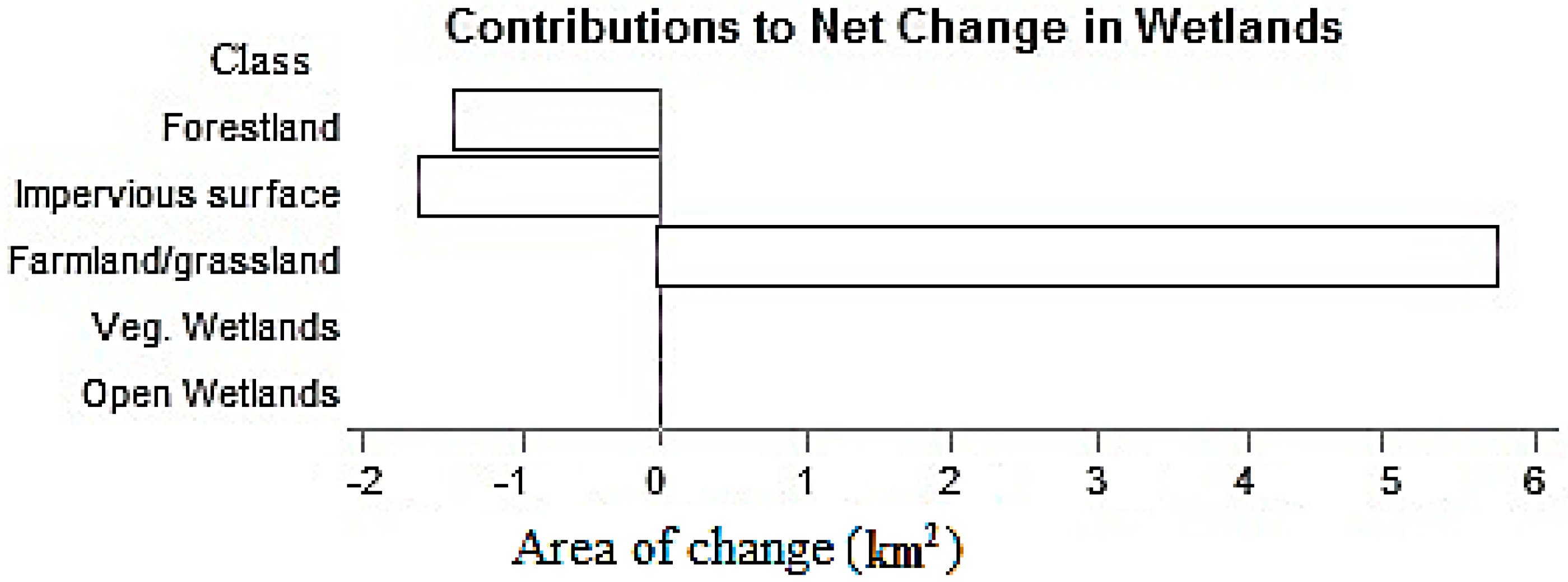
We examined the contributions to net change in wetlands between these periods (Figure 7) and found that impervious surfaces had the highest contribution to the loss experienced in wetlands followed by forestland, respectively. Findings from a similar study [2] also showed urban expansion played a significant role in the reduction of vegetated wetlands. Figure 7 clearly showed impervious surfaces and forestland are the two classes with notable increases, which is at the expense of both wetlands and farmlands/grasslands (Figure 7).
To examine which watershed is experiencing the loss in vegetated wetlands, Tables 9–11 show that the Blue River watershed was the only watershed where wetlands were lost between 1992 and 2010. These tables also show that the highest increase in impervious surfaces occurred in the Blue River watershed.
3.2. Modeling the Potential for Change
Based on the 11 land change driving variables selected and the land cover maps of 1992 and 2010, this study investigated the potential for land to change within the three watersheds using the similarity weighted instance-based machine learning model. Six transitions earlier discussed in the methods section were modeled using this method. Table 5 showed the goodness of fit of the model. The hit rate and the false alarm represent the goodness of fit of the model. A high hit rate signifies a high potential for change in areas that actually changed, and the Peirce Skill is the difference between the hit rate and the false alarm. The breakdown of the model parameter in Table 5 revealed high hit rates for the six transitions modeled. This indicates that there is a high potential that the transitions that were modeled will occur.
Relevance weight (Figure 8) for the conversion of wetlands to farmlands and impervious surfaces showed that the likelihood for the land to change, distances from already disturbed lands and already urbanized areas played the most significant roles in the conversion process. This is mostly for economic purposes. It is more economical to develop close to already disturbed areas than developing in undisturbed areas. Relevance weights are an indication of these variables’ importance in the model. A high variable weight means a greater importance.
Using impervious surfaces as an index of urban development, the study revealed the dynamics of wetland loss to urban expansion in the study area. Open wetlands were not included in the transition modeling because when we looked at the net change in this category between 1992 and 2010, the result showed an increase between these periods but a decrease in vegetated wetlands (Figure 7). Nevertheless, because the increase in open wetlands was more than the vegetated wetlands, the overall outlook of wetlands when combined revealed an increase, which can be misleading; hence, we examined both types of wetlands independently.
3.3. Integration with Markov Chain for Change Prediction and Validation
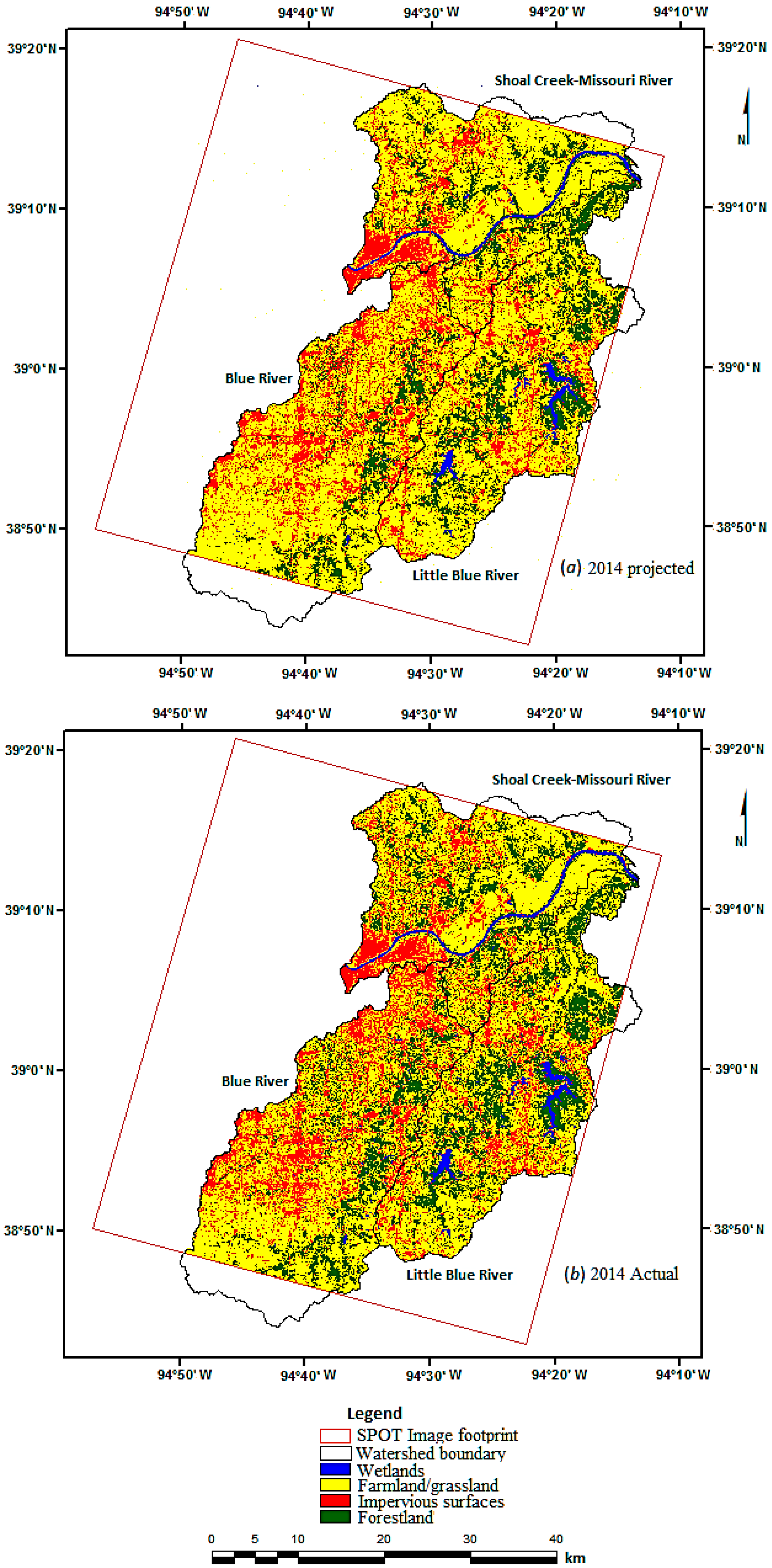
We compared and validated predictions for 2014 from SimWeight model with an independently classified land cover map of 2014. Figure 9 showed the actual land cover map of 2014 (Figure 9a) and the predicted land cover map (Figure 9b).
Table 6 is the associated accuracy assessment for the actual and predicted land cover maps of 2014. The accuracies of both maps reveal the differences in land cover statistics between the two maps, which demonstrated how the model performed (Table 6). The proportion of pixels correctly and incorrectly predicted, producer and user’s accuracies are also included in the table. Producer’s accuracy corresponds to the error of omission, i.e., exclusion—pixels that belong to a category, e.g., wetlands, are incorrectly predicted as other categories, e.g., forestland. User’s accuracy corresponds to the error of commission, i.e., inclusion—pixels that belong to other categories, e.g., grassland/farmlands, are incorrectly allocated to the category under examination. In this case, the table showed higher percentages in the producer and user’s accuracies of the actual map than in the projected map (which is expected), except for wetlands, which has a higher producer’s accuracy for the predicted map than the actual map. This implied that more pixels were correctly allocated to wetlands in the predicted map than in the actual map, which is good for the purpose of our study. Overall, the errors in each class of the predicted map may propagate into future prediction; thus, this study considers the predicted map for 2014 a satisfactory basis for making future prediction [1].
Results from validating the predicted map with the independent map shows that both maps had a match of 1197.17 km2 corresponding to 75.6% and a miss of 385.71 km2 corresponding to 24.4%. The overall accuracy of the modeled map differs by about 10.0% when compared to the actual map (Table 6). This match between the land cover categories of the predicted map and the actual map, and the over 80% accuracy obtained on the predicted map suggested that the model can be used as a basis for modeling into the future.
3.4. Landscape Projection into 2028
To assess the future impacts of urban expansion-induced landscape change on wetlands within the watersheds under study, landscape within the watersheds were projected into 2028 using the already calibrated model. Analysis of change was carried out for all three watersheds studied. Figure 10 is the projected map with the associated table (Table 7).
3.5. Change Analysis on the Landscape between 1992 and 2028
We analyzed change between 1992 and 2028 in the three watersheds combined. A closer look at the watersheds revealed that there are different dynamics of change, particularly with wetlands. Analysis of change in wetlands between 1992 and 2010 in the three watersheds combined revealed an increase in this class, but a projected decrease between 2010 and 2028 (Table 8). Unfortunately, this obscures the change dynamics at a smaller scale. When we examined and interpreted our result at the individual watershed scale, we found that wetlands were actually lost in one watershed (Blue River watershed) between 1992 and 2010. This would have gone unnoticed without a closer look at the individual watersheds. Analysis of change in the other classes such as farmlands/grasslands showed a decrease of 16.2% between 1992 and 2010 (Table 8). In addition, projections into 2028 revealed that this decrease will likely continue into the future, but the magnitude would reduce. An assessment of change between 1992 and 2028 revealed the possibility of continued reduction in farmlands/grasslands by 23.8%. While forestland increased between 1992 and 2010, the predicted forest cover of the area suggested a possible reduction. Nevertheless, this reduction would be minimal when examined between 1992 and 2028. For impervious surfaces, the increase experienced between 1992 and 2010 may likely continue into the future with approximately the same magnitude.
A closer look at the overall patterns of change (1992 and 2028) and changes within the overall period (1992 and 2010, and 2010 and 2028) revealed the temporal dimensions of change. When the results of the change analysis between 1992 and 2028 in the Blue River watershed were examined (Table 9), we observed wetland loss in this watershed between 1992 and 2010, but was projected to not change in percent coverage between 2010 and 2028. This can be misleading because an examination of wetland acreage suggests a continued decline. As mentioned earlier, this decline can be mainly attributed to vegetated wetlands, which is more susceptible to the effects of urban expansion. Farmlands/grasslands experienced a reduction similar to what occurred in the three watersheds combined. Between 1992 and 2010, farmlands/grasslands decreased by 16.0%. Although this reduction will likely continue into the future, it was projected that the amount of reduction in this class will slow down between 2010 and 2028.
Forestland increased between 1992 and 2010, but was projected to decrease slightly between 2010 and 2028. Overall, between 1992 and 2010, it was projected that forestland would gain 4.3% area coverage. On the other hand, projected changes in impervious surfaces between 2010 and 2028 will be similar to what took place between 1992 and 2010. This is an increase as expected. It was projected that, between 1992 and 2028, the change will be 27.3%. This is a huge growth in impervious surfaces compared to the other classes, which is expected considering that there has been a population influx into the Kansas City area in the last two decades. The Kansas City Metro area experienced an estimated growth rate of about 11.3% between 2000 and 2010 [27].
As with the Blue River watershed, farmland/grassland experienced a reduction between 1992 and 2010 in the Little Blue River watershed (Table 10), and the projected change in this class indicated that the reduction will continue between 2010 and 2028. An analysis of change between 1992 and 2028 suggested a projected decrease of about 24.5%. This revealed that farmland/grassland is very susceptible to change. This class has the largest reduction in this watershed, which can be attributed to a rapid urban expansion. Indeed, this is the case in all three watersheds. In contrast, forestland increased between 1992 and 2010. However, based on our projections, the size of this class will decrease by 2028. Forestland loss may be minimal, but it requires attention so that the historical gains will not be lost. Projections in forestland between 1992 and 2028 show an increase of about 13.5% (Table 10). Impervious surfaces are expected to increase by 3.7% between 1992 and 2010, and are projected to experience an increase of 7.3% between 2010 and 2028. Between 1992 and 2028, it is expected that impervious surfaces will increase by about 11.0%. Wetlands (open and vegetated) increased between 1992 and 2010, but were projected to reduce by 2028. As mentioned before, the increase was mainly in open wetlands. Vegetated wetlands experienced a decline historically and may continue to experience this in the future.
We examined the result of change analysis in the Shoal Creek-Missouri River watershed between 1992 and 2028 (Table 11). The pattern of change in this watershed is similar to that of the Little Blue River watershed. Farmland/grassland lost between 1992 and 2010, and was projected to lose also between 2010 and 2028. An overall reduction of 22.3% is expected between 1992 and 2028. Forestland increased by 11.0% between 1992 and 2010, but was projected to slightly decline between 2010 and 2028. An overall examination of forestland between 1992 and 2028 revealed that forestland would maintain an increase of about 10.0%. Impervious surfaces increased by 5.0% between 1992 and 2010, and are expected to keep increasing between 2010 and 2028. This translated to a projected increase of 12.1% between 1992 and 2028. Wetlands increased between 1992 and 2010, but are projected to remain the same between 2010 and 2028 percent wise. This can be misleading because an examination of wetland acreage suggested a continued decline between these periods.
3.6. Analysis of Wetlands Loss to Urban Expansion within the Three Watersheds
We used the magnitude of wetland loss to impervious surfaces as an index of urban expansion to determine the impact of human-induced landscape change on wetlands in the study area. In general, this study observed that most of the losses experienced in the study area involved the changes to impervious surfaces. This suggested that the area is experiencing a rapid urban expansion. However, for wetlands in particular, while there was a net increase overall, about 1.31 km2 of wetland (mostly vegetated wetlands) were lost to impervious surfaces in the entire study area between 1992 and 2010. It was projected that the amount of wetland loss to impervious surfaces may reduce to about 1.11 km2 between 2010 and 2028.
Analysis of wetland loss to impervious surfaces in each watershed within the study area showed various patterns of loss at a smaller scale (Table 12). We observed that about 0.7 km2 of wetlands were lost to impervious surfaces between 1992 and 2010 in the Blue river watershed (which is the largest in all the three watersheds) and about 0.02 km2 between 2010 and 2028. This will reduce the amount of wetland loss in this watershed, when compared to what happened previously. Similarly, the Shoal Creek-Missouri River watershed showed a similar pattern of possible reduction in wetlands that may be lost to impervious surfaces by 2028. About 0.2 km2 of wetland was lost to impervious surfaces between 1992 and 2010 in the Shoal Creek-Missouri River watershed. Nevertheless, by 2028, the magnitude of the reduction will be reduced to 0.13 km2. Unfortunately, the situation may be different in the Little Blue River watershed. The analysis of wetland loss to impervious surfaces in the Little Blue River watershed (Table 12) revealed that the amount of decrease between 2010 and 2028 might actually increase in this particular watershed when compared to the decrease between 1992 and 2010. Despite these observations, we must not forget that this reduction is majorly in the vegetated wetlands. Overall, the result indicated that the Blue River watershed has historically been more susceptible to urban expansion when compared to the other two watersheds. Future projections indicated that the Little Blue River watershed might be the most susceptible of the three.
4. Discussion
A general assessment of landscape change in the study area revealed a remarkable loss in farmland/grassland. However, the trend of the reduction in farmland/grassland experienced historically in the study area is not new. Many urban landscapes around the world have experienced similar reduction (e.g., [44,45,46]). Ji et al. [2] found that there was a large loss in farmland/grassland. What is more concerning is the projections from our study that revealed continued loss in the future. Projections from this study revealed a continued reduction in farmland/grassland into the future at a remarkable amount. While conversion of grassland into other uses is typical of many urban environments, efforts should be made at conserving the farmlands, which can help support the urban population. On the other hand, while forestland increased historically, this study projected that this trend may not continue into the future except where deliberate attempts are made to sustain the increase experienced historically.
Wetlands, a focus of this study, have different patterns of change in all three watersheds. For instance, wetlands increased historically in the Shoal-Creek Missouri River and Little Blue river watersheds, but lost in the Blue River watershed. Our results indicate that the loss of wetland area coincides with rapid urban expansion. Results from this study showed both impervious surfaces and forestlands are the two classes that replaced vegetated wetlands (Figure 7). It is therefore evident that vegetated wetlands need more attention than open wetland because of their susceptibility to change that is a result of urban development.
According to the study projections, urban expansion would continue into the future, following historical patterns. This would be expected considering the population increase trend that was experienced in the Kansas City area in the past [28], and the future projections given by the Mid-America Regional Council (MARC), which revealed that the population of the area may grow by 582,000 people between 2010 and 2040 [31]. In the long run, this increase will translate into more lands (including wetland areas) being developed in the Kansas City area. Historically, there was a net increase in wetlands between 1992 and 2010 in two watersheds, while there was a reduction in one watershed (the Blue River Watershed). Projections into 2028 revealed that wetlands might lose in all three watersheds in the future. Similar results have been observed in a recent study in which, human induced factors such as pollution and particularly, construction were the predominant causes for wetland changes historically, and potential cause in the future [47].
When we compared the amount of wetland loss to impervious surfaces between 1992 and 2010 and between 2010 and 2028, we observed that the magnitude of loss will reduce in both the Blue River Watershed and the Shoal Creek-Missouri-River between 2010 and 2028, but may actually increase in the Little Blue River Watershed. Based on these projections, we recommend that closer attention should be given to wetlands in the Little Blue River watershed, where urban expansion may make wetlands more susceptible to change in the future. Our results indicate that vegetated wetland has been, and will continue to be more susceptible to the negative impacts of urbanization. This suggests the need for an increased effort in conserving vegetated wetlands in the study area.
To determine if the projected decline in wetlands can solely be attributed to urban expansion without the influence of climate variability, this study obtained the United States Global Change Research Program’s (USGCRP) projections of precipitation and storm events given for the Mid-Western Region (including the States of Missouri and Kansas) by Thomas et al. [48]. According to these reports, observations of average precipitation and storm events between 1993 and 2008 suggest that the annual mean precipitation has increased by 5.0% relative to the 1962–1979 period [48]. Further, projections of precipitation between 2010 and 2040 for the area revealed a potential increase of between 6.0% to 7.0%, especially in the winter months, and a likely range of +2 to +12% [48]. Although, when we consider other complex factors such as frequency and rate of precipitation, run off potential, temperature and evapotranspiration rates, projections of variability in precipitation and storm water events may be a simplified approach to assessing the amount of land that is wet. Nevertheless, these results suggest that climate variability may not account for the projected decrease in wetlands in the study area. Based on these projections, we conclude that the likely reduction in wetlands will be mainly human-induced, suggesting that proper planning activities should be done at all levels to mitigate against this potential decline.
5. Conclusions
This study examined the impact of human-induced landscape change on urban wetlands in three major watersheds in the Kansas City area, between 1992 and 2010. Findings reveal that wetlands increased in two watersheds historically, but lost to urban expansion in one. Further, future projections reveal that wetlands may lose to urban expansion in all three watersheds in the future, particularly, the Little Blue River watershed. This study demonstrated the possibility of simulating the impacts of human-induced landscape change on urban wetlands using an integrated approach. This modeling approach in combination with land change driving variables provided insights about how urban landscape may develop in the study area and how this development may affect urban ecosystems such as wetlands. This modeling approach can serve as a vital tool in wetland conservation and sustainability.
Acknowledgments
This work utilized SPOT satellite imageries that were acquired through the previous study of urban wetland changes in the study area, which was supported by the US EPA Grant CD 97701501 and by the grant of the Friends of the Library of the University of Missouri—Kansas City.
Author Contributions
Opeyemi A. Zubair and Wei Ji conceived and designed the experiments; Opeyemi A. Zubair performed the experiments; Opeyemi A. Zubair analyzed the data; Opeyemi A. Zubair and Wei Ji contributed reagents/materials/analysis tools; and Opeyemi A. Zubair, Wei Ji and Trina Weilert wrote the paper.
Conflicts of Interest
The authors declare no conflict of interest. The founding sponsors had no role in the design of the study; in the collection, analyses, or interpretation of data; in the writing of the manuscript, and in the decision to publish the results.
References
- Zubair, O.A.; Ji, W. Assessing the Impact of Land Cover Classification Methods on the Accuracy of Urban Land Change Prediction. Can. J. Remote Sens. 2015, 41, 170–190. [Google Scholar] [CrossRef]
- Ji, W.; Xu, X.; Murambadoro, D. Understanding urban wetland dynamics: Cross-scale detection and analysis of remote sensing. Int. J. Remote Sens. 2015, 36, 1763–1788. [Google Scholar] [CrossRef]
- Kienast, F.; Bolliger, J.; Potschin, M.; de Groot, R.S.; Verburg, P.H.; Heller, I.; Wascher, D.; Haines-Young, R. Assessing Landscape Functions with Broad-Scale Environmental Data: Insights Gained from a Prototype Development for Europe. Environ. Manag. 2009, 44, 1099–1120. [Google Scholar] [CrossRef] [PubMed]
- Luck, M.; Wu, J. A gradient analysis of the landscape pattern of urbanization in the Phoenix metropolitan area of USA. Landsc. Ecol. 2002, 17, 327–339. [Google Scholar] [CrossRef]
- Masek, J.G.; Lindsay, E.F.; Goward, N.S. Dynamics of urban growth in the Washington DC metropolitan area, 1973–1996, from Landsat observations. Int. J. Remote Sens. 2000, 21, 3473–3486. [Google Scholar] [CrossRef]
- Otero, I.; Boada, M.; Varga, D. Consequences of the transition from primary to a tertiary landscape in Olzinelles (NE Spain), 1853–2008. In Proceedings of the European IALE Conference, Salzburg, Austria/Bratislava, Slovakia, 12–16 July 2009; pp. 80–84. [Google Scholar]
- Pauleit, S.; Breuste, J.; Qureshi, S.; Sauerwein, M. Transformation of rural-urban landscapes in Europe: Integrating approaches from ecological, socio-economic and planning perspectives. Landsc. Online 2010, 20, 1–10. [Google Scholar] [CrossRef]
- Turner, M.G. Landscape ecology: The effects of pattern on process. Ann. Rev. Ecol. Syst. 1989, 20, 171–197. [Google Scholar] [CrossRef]
- Vogiatzakis, I.; Pungetti, G.; Makhzoumi, J. Mediterranean island landscapes’ transformation: The past 50 years. In Proceedings of the European IALE Conference, Salzburg, Austria/Bratislava, Slovakia, 12–16 July 2009; pp. 108–111. [Google Scholar]
- Whitehand, J.W.R. The Changing Urban Landscape: The Case of London’s High-Class Residential Fringe. Geogr. J. 1988, 154, 351–366. [Google Scholar] [CrossRef]
- Jones, K.B.; Neale, A.C.; Wade, T.G.; Wickham, J.D.; Cross, C.L.; Edmonds, C.M.; Loveland, T.R.; Nash, M.S.; Riitters, K.H.; Smith, E.R. The consequences of landscape change on ecological resources: an assessment of the United States Mid-Atlantic Region, 1973–1993. Ecosyst. Health 2001, 7, 229–242. [Google Scholar] [CrossRef]
- Mehaffey, M.; Smith, E.; Van Remortel, R. Midwest U.S. landscape change to 2020 driven by biofuel mandates. Ecol. Appl. 2012, 22, 8–19. [Google Scholar] [CrossRef] [PubMed]
- García, A.M.; Santé, I.; Boullón, M.; Crecente, R. A comparative analysis of cellular automata models for simulation of small urban areas in Galicia, NW Spain. Comput. Environ. Urban Syst. 2012, 36, 291–301. [Google Scholar] [CrossRef]
- He, C.; Okada, N.; Zhang, Q.; Shi, P.; Li, J. Modeling dynamic urban expansion processes incorporating a potential model with cellular automata. Landsc. Urban Plan. 2008, 86, 79–91. [Google Scholar] [CrossRef]
- Huang, W.; Liu, H.; Luan, Q.; Jiang, Q.; Liu, J.; Liu, H. Detection and prediction of land use change in Beijing based on remote sensing and GIS. Int. Arch. Photogramm. Remote Sens. Spat. Inf. Sci. 2008, 37, 75–82. [Google Scholar]
- Li, X.; Yeh, A. Modeling sustainable urban development by the integration of constrained cellular automata and GIS. Int. J. Geogr. Inf. Sci. 2000, 14, 131–152. [Google Scholar] [CrossRef]
- Li, X.; Yeh, A. Neural-network-based cellular automata for simulating multiple land use changes using GIS. Int. J. Geogr. Inf. Sci. 2002, 16, 323–343. [Google Scholar] [CrossRef]
- Kauffman, G.J.; Brant, T. The Role of Impervious Cover as a Watershed-based Zoning Tool to Protect Water Quality in the Christina River Basin of Delaware, Pennsylvania, and Maryland. In Proceedings of the Watershed Management, Tucson, AZ, USA, 13–16 January 2000; University of Delaware: Newark, NJ, USA, 2000; pp. 1–16. [Google Scholar]
- US Environmental Protection Agency (USEPA). Functions and Values of Wetlands. 2006. Available online: http://water.epa.gov/type/wetlands/upload/2006_08_11_wetlands_fun_val.pdf (accessed on 18 November 2015).
- US Environmental Protection Agency (USEPA). Wetland Fact Sheet. 2012. Available online: http://water.epa.gov/type/wetlands/outreach/facts_contents.cfm (accessed on 10 September 2015).
- US Environmental Protection Agency (USEPA). Wetlands—Status and Trends. 2012. Available online: http://water.epa.gov/type/wetlands/vital_status.cfm (accessed on 18 November 2015).
- Copeland, C. Wetlands: An Overview of Issues. Congressional Research Service Report 2013. Available online: http://nationalaglawcenter.org/wp-content/uploads/assets/crs/RL33483.pdf (accessed on 3 November 2015).
- Wang, X.; Ning, L.; Yu, J.; Xiao, R.; Li, T. Changes of Urban Wetland Landscape Pattern and Impacts of Urbanization on Wetland in Wuhan City. Chin. Geogr. Sci. 2008, 18, 47–53. [Google Scholar] [CrossRef]
- Sangermano, F.; Eastman, J.R.; Zhu, H. Similarity Weighted Instance-based Learning for the Generation of Transition Potentials in Land Use Change Modeling. Trans. GIS 2010, 14, 569–580. [Google Scholar] [CrossRef]
- Weng, Q. Land use change analysis in the Zhujiang Delta of China using satellite remote sensing, GIS and stochastic modeling. J. Environ. Manag. 2002, 64, 273–284. [Google Scholar] [CrossRef]
- Guan, D.; Li, H.; Inohae, T.; Su, W.; Nagaie, T.; Hokao, K. Modeling urban land use change by the integration of cellular automaton and Markov chain. Ecol. Model. 2011, 222, 3761–3772. [Google Scholar] [CrossRef]
- MARC (Mid-America Regional Council). Census 2010: Census Data for the MARC Region. 2014. Available online: http://www.marc.org/Data-Economy/Metrodataline/Population/Census-2010 (accessed on 21 September 2017).
- Ji, W.; Ma, J.; Twibell, W.R.; Underhill, K. Characterizing urban sprawl using multi-stage remote sensing images and landscape metrics. Comput. Environ. Urban Syst. 2006, 30, 861–879. [Google Scholar] [CrossRef]
- The Brookings Institution. Growth in the Heartland: Challenges and Opportunities for Missouri 2002; The Brookings Institution Center on Urban and Metropolitan Policy: Washington, DC, USA, 2002; Available online: http://www.brookings.edu/~/media/research/files/reports/2002/12/missouri/missouri.pdf (accessed on 21 September 2017).
- Song, C.; Woodcock, E.C.; Seto, C.K.; Lenney, P.A.; Macomber, A.S. Classification and Change Detection Using Landsat TM Data: When and How to Correct Atmospheric Effects? Remote Sens. Environ. 2001, 75, 230–244. [Google Scholar] [CrossRef]
- Jensen, J.R. Introductory to Digital Image Processing: A Remote Sensing Perspective, 4th ed.; Prentice Hall: Upper Saddle River, NJ, USA, 2015; pp. 365–453. [Google Scholar]
- MARC (Mid-America Regional Council). Technical Forecast Process. 2014. Available online: http://www.marc.org/Data-Economy/Forecast/Forecast-Process/Overview (accessed on 21 September 2017).
- Tso, B.; Mather, M.P. Classification Methods for Remote Sensing Data; Taylor & Francis: London, UK, 2001. [Google Scholar]
- IDRISI Focus Paper, “The Land Change Modeler for Ecological Sustainability 2009”. Available online: http://clarklabs.org/applications/upload/Land-Change-Modeler-IDRISI-Focus-Paper.pdf (accessed on 21 September 2017).
- Gómez, O.; Morales, E.F.; González, J.A. Weighted Instance-based learning using representative intervals. In Advances in Artificial Intelligence, Proceedings of the Sixth Mexican International Conference on Artificial Intelligence, Aguascalientes, Mexico, 4–10 November 2007; Gelbukh, A., Morales, K., Fernando, A., Eds.; Lecture Notes in Computer Science; Volume 4827, pp. 420–430. Available online: http://www.isprs.org/proceedings/XXXVII/congress/6b_pdf/13.pdf (accessed on 21 September 2017).
- Mozumber, C.; Tripathi, N.K.; Losiri, C. Comparing three transition potential models: A case study of built-up transitions in North-East India. Comput. Environ. Urban Syst. 2016, 59, 38–49. [Google Scholar] [CrossRef]
- Eastman, J.R.; Solorzano, L.A.; Van Fossen, M. Transition potential modeling for land-cover change. In GIS, Spatial Analysis and Modelling; Maguire, D.J., Batty, M., Goodchild, M.F., Eds.; ESRI Press: Redlands, CA, USA, 2005; pp. 357–385. [Google Scholar]
- Baker, W.L. A review of models of landscape change. Landsc. Ecol. 1989, 2, 111–133. [Google Scholar] [CrossRef]
- Arsanjani, J.J.; Helbich, M.; Kainz, W.; Boloorani, D.A. Integration of logistic regression, Markov chain and cellular automata models to simulate urban expansion. Int. J. Appl. Earth Obs. Geoinf. 2013, 21, 265–275. [Google Scholar] [CrossRef]
- Zhang, R.; Tang, C.; Ma, S.; Yuan, H.; Gao, L.; Fan, W. Using Markov chains to analyze changes in wetland trends in arid Yinchuan Plain, China. Math. Comput. Model. Agric. 2011, 54, 924–930. [Google Scholar] [CrossRef]
- Sangermano, F.; Toledano, J.; Eastman, J.R. Land cover change in the Bolivian Amazon and its implications for REDD+ and endemic biodiversity. Landsc. Ecol. 2012, 27, 571–584. [Google Scholar] [CrossRef]
- Eastman, J.R.; Jin, W.; Kyem, P.A.K.; Toledano, J. Raster Procedures for Multi-Criteria/Multi-Objective Decisions. Photogramm. Eng. Remote Sens. 1995, 61, 539–547. [Google Scholar]
- Senseman, M.G.; Calvin, B.F.; Tweddale, S.A. Accuracy Assessment of the Discrete Classification of Remotely-Sensed Digital Data for Land Cover Mapping; USACERL Technical Report EN-95/04; USACERL: Champaign, IL, USA, 1995; pp. 1–35. Available online: http://www.dtic.mil/get-tr-doc/pdf?AD=ADA296212 (accessed on 22 September 2017).
- López, M.T.; Aide, T.M.; Thomlinson, R.J. Urban Expansion and the Loss of Prime Agricultural Lands in Puerto Rico. Ambio 2001, 30, 49–54. [Google Scholar] [CrossRef] [PubMed]
- Liu, Y.; Yang, Y.; Li, Y.; Li, J. Conversion from rural settlements and arable land under rapid urbanization in Beijing during 1985–2010. J. Rural Stud. 2017, 51, 141–150. [Google Scholar] [CrossRef]
- Vliet, J.; Eitelberg, A.D.; Verburg, H.P. A global analysis of land take in cropland areas and production displacement from urbanization. Glob. Environ. Chang. 2017, 43, 107–115. [Google Scholar] [CrossRef]
- Ma, C.; Zhang, Y.G.; Zhang, C.X.; Zhao, J.Y.; Li, Y.H. Application of Markov model in wetland change dynamics in Tianjin Coastal Area, China. Procedia Envion. Sci. 2010, 13, 252–262. [Google Scholar] [CrossRef]
- Karl, R.T.; Melillo, M.J.; Peterson, C.T. Global Climate Changes Impacts in the United States; United States Global Change Research Program (USGCRP), Ed.; Cambridge University Press: New York, NY, USA, 2009; pp. 117–122. Available online: https://downloads.globalchange.gov/usimpacts/pdfs/climate-impacts-report.pdf (accessed on 22 September 2017).
Figure 1.
Map of the study area that included nine counties of the 14-county Kansas City metropolitan area.
Figure 1.
Map of the study area that included nine counties of the 14-county Kansas City metropolitan area.

Figure 2.
Flow chart of the major methods in this study.

Figure 3.
Spectral Profiles of the three SPOT images classified for this study.
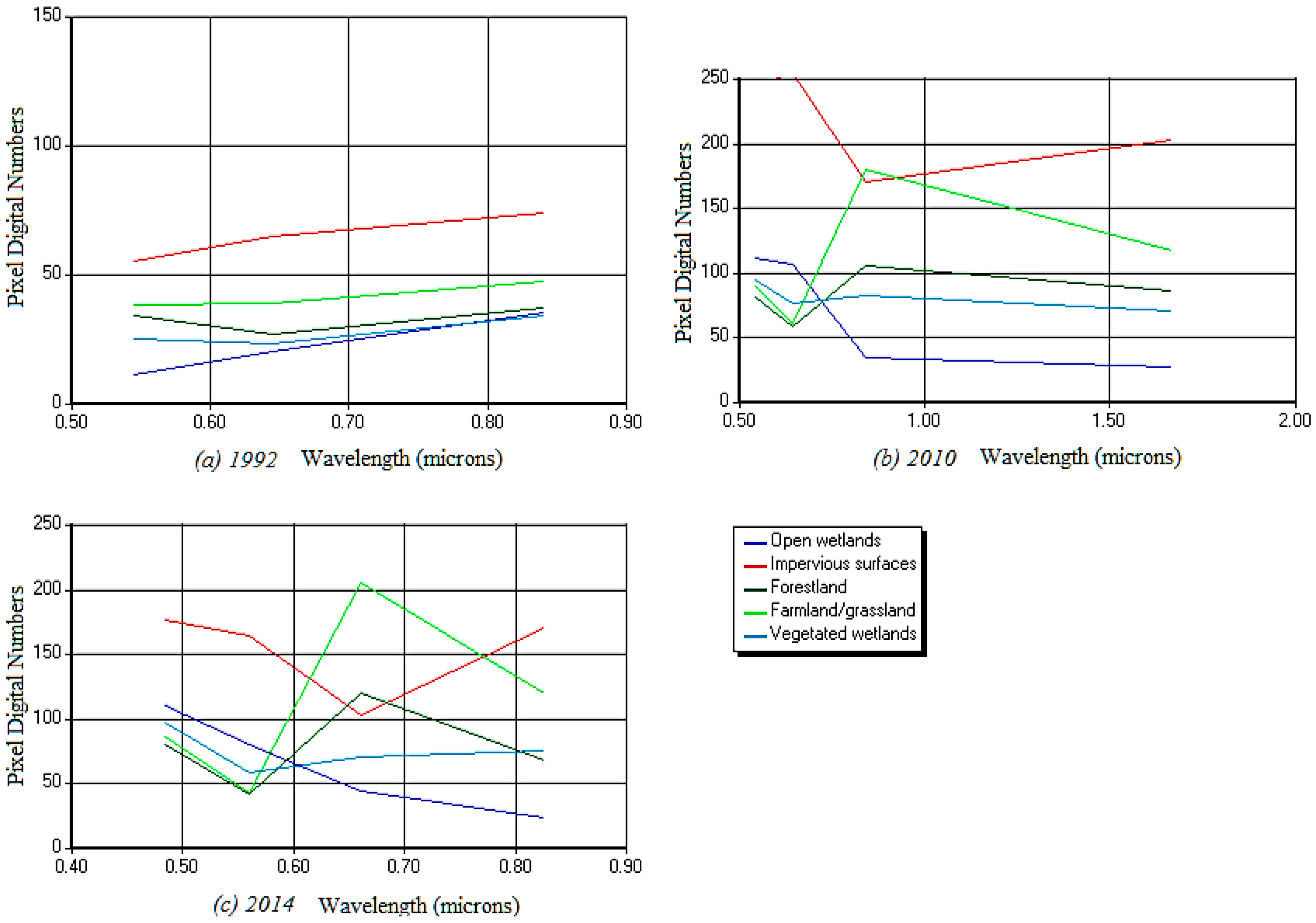
Figure 4.
Kansas City land cover of the three major watersheds in 1992 and 2010.

Figure 5.
Increase and decrease between 1992 and 2010 land cover maps.
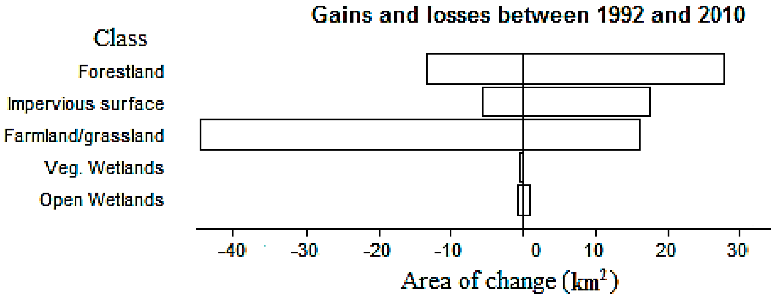
Figure 6.
Net change between 1992 and 2010 land cover classes.
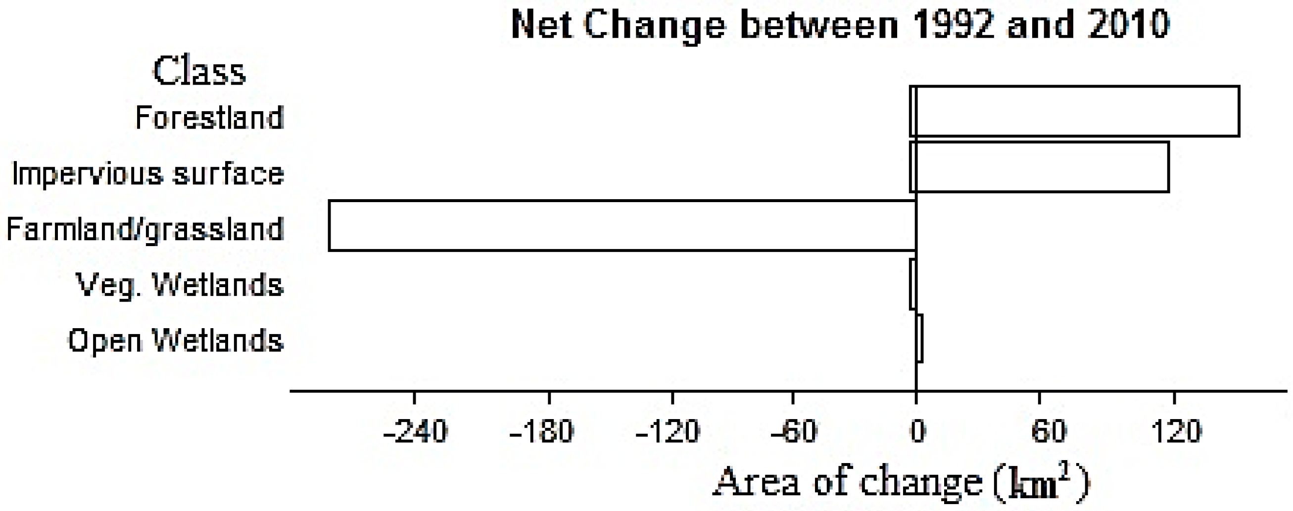
Figure 7.
Contributions to net change in wetlands between 1992 and 2010.

Figure 8.
Relevance of the change variables based on transitions from wetlands to farmlands and impervious surfaces.
Figure 8.
Relevance of the change variables based on transitions from wetlands to farmlands and impervious surfaces.

Figure 9.
Land cover map and projected land cover map of Kansas City major watersheds in 2014.

Figure 10.
Projected land cover maps of Kansas City major watersheds in 2028.

Table 1.
Characteristics of SPOT images.
| Sensor | Date | Scene ID | Spectral Mode | No. of Bands | Processing Level | Spatial Resolution (m) | Source |
|---|---|---|---|---|---|---|---|
| SPOT 2 | 29 January 1992 | 2 587-272 92-01-29 17:23:19 2 X | XS | 3 | 1A | 20 | SPOT image corporation |
| SPOT 5 | 10 August 2010 | 5 586-271/5 10/08/10 17:12:31 1 J | J | 4 | 2A | 10 | SPOT image corporation |
| SPOT 5 | 14 August 2014 | 5 586-271/3 14/08/20 16:35:21 1 J | J | 5 | 2A | 10 | Astrium GEO-information services North America |
Table 2.
Characteristics of the driving variables, sources, and datasets from which they were derived.
Table 2.
Characteristics of the driving variables, sources, and datasets from which they were derived.
| Dataset | Year | Source | Description | Derived Variable | Spatial Resolution (m) |
|---|---|---|---|---|---|
| Roads | 2010 | United States Census Bureau | Interstate highways, state highways, US highways, and marginal/service roads in shapefile format | Distance from roads | 20 |
| Land cover maps | 1992, 2010 | SPOT images of the study area in 1992, 2010 | Obtained from classifying the SPOT images of 1992 and 2010 | Land cover likelihoods | 20 |
| Streams | 2010 | United States Census Bureau | Streams in the Kansas City area, with stream order and stream name | Distance from streams | 20 |
| Land cover maps | 2010 | SPOT image of the study area in 2010 | Urban areas on the land cover maps in 2010 | Distance from urban areas | 20 |
| Land cover maps | 1992 | SPOT image of the study area in 1992 | An extraction of all the previously disturbed areas on the 1992 classified map | Distance from anthropogenic disturbances | 20 |
| National Elevation Data (NED) | 2014 | US Geological Survey National Elevation Dataset (NED) | NED came with 10 m spatial resolution in tiff format. This was processed to 20 m resolution | NED | 20 |
| National Elevation Data (NED) | 2014 | US Geological Survey National Elevation Dataset (NED) | Slope was derived from NED in degrees | Slope | 20 |
| Park and ride | 2010 | Mid-America Regional Council | Park-and-ride locations in the Kansas City area in shapefile format, where motorists can park and connect to transit or carpool | Distance from park and ride | 20 |
| Parks and recreation | 2009–2010 | Center for Economic Development, UMKC | Parks, playgrounds, camping sites, sports courts, skate parks, golf courses etc. in shapefile format | Distance from parks and recreation | 20 |
| Population data | 2010 | Mid-America Regional Council (MARC) | 2010 population data of Kansas City area by block in shapefile format | Population | 20 |
| Central business district | 2010 | Center for Economic Development, University of Missouri-Kansas City, Missouri. | The central business district of Kansas City area in shapefile format | Distance from Kansas City central business district | 20 |
Table 3.
Incentives and constraints datasets used in this study.
| Dataset | Year | Source | Description |
|---|---|---|---|
| Protected areas | 2009–2012 | United States Geological Survey’s Protected Area Database of the United States | A geodatabase that illustrates and describes public land ownership, nationally conserved lands nationally, and privately protected areas that were provided voluntarily |
| Tax incentive areas to encourage development | 2009 | Missouri Dept. of Economic Development, Missouri Economic Research and Information Center | Distressed communities where Tax Credit were given to encourage development projects |
| Watershed boundaries | 2010 | Missouri Natural Resources Conservation Service | Boundaries of delineated watershed and sub-watershed areas in Kansas City area |
Table 4.
Accuracy assessment of the classified images obtained from a previous study (Ji et al., 2015).
Table 4.
Accuracy assessment of the classified images obtained from a previous study (Ji et al., 2015).
| Accuracy Assessment | ||||||
|---|---|---|---|---|---|---|
| Land Cover Class | Area (%) | 1992 | 2010 | |||
| Accuracy Assessment (%) | ||||||
| 1992 | 2010 | Producer’s | User’s | Producer’s | User’s | |
| Farmland/grassland | 77.5 | 61.2 | 88.7 | 93.4 | 87.8 | 94.3 |
| Forestland | 14.3 | 23.6 | 94.8 | 87.3 | 96.4 | 84.0 |
| Impervious surfaces | 6.4 | 13.5 | 91.5 | 86.1 | 95.2 | 97.2 |
| Wetland | 1.9 | 2.0 | 92.1 | 90.3 | 94.9 | 93.0 |
| Total | 100.0 | 100.0 | ||||
| Overall classification accuracy | 90.1 | 91.8 | ||||
Table 5.
Breakdown of the model parameter results for each transition.
| Transition | Sample Size | K | Hit Rate | False Alarm | Peirce Skill Score |
|---|---|---|---|---|---|
| Open wetlands to vegetated wetlands | 46 | 10 | 0.8 | 0.2 | 0.6 |
| Vegetated wetlands to farmland/grassland | 1000 | 100 | 0.9 | 0.0 | 0.9 |
| Vegetated wetlands to impervious surface | 692 | 69 | 0.9 | 0.0 | 0.9 |
| Farmland/grassland to impervious surface | 1000 | 100 | 0.9 | 0.0 | 0.9 |
| Forestland to farmland/grassland | 1000 | 100 | 0.9 | 0.0 | 0.9 |
| Forestland to impervious surface | 1000 | 100 | 0.9 | 0.0 | 0.9 |
Table 6.
Accuracy assessment of the projected land cover map and the actual map.
| Accuracy Assessment | ||||||
|---|---|---|---|---|---|---|
| Land Cover Class | Projected | Actual | 2014 Projected | 2014 Actual | ||
| Area (%) | Accuracy Assessment (%) | |||||
| 2014 | 2014 | Producer’s | User’s | Producer’s | User’s | |
| Farmland/grassland | 56.8 | 56.8 | 89.6 | 82.2 | 95.5 | 90.1 |
| Forestland | 23.0 | 22.3 | 64.7 | 81.4 | 87.3 | 85.7 |
| Impervious surfaces | 18.5 | 18.9 | 97.6 | 71.7 | 86.8 | 97.9 |
| Wetland | 1.8 | 2.0 | 66.7 | 100.0 | 62.5 | 100.0 |
| Total | 100.0 | 100.0 | ||||
| Overall classification accuracy | 80.4 | 90.8 | ||||
Table 7.
Area of projected land cover in 2028.
| Area of Projected Land Cover in the Three Study Watersheds Combined | ||
|---|---|---|
| Land Cover Class | 2028 | |
| km2 | Area (%) | |
| Farmland/grassland | 925.61 | 53.9 |
| Forestland | 392.42 | 23.1 |
| Impervious surfaces | 372.41 | 21.1 |
| Wetland | 32.56 | 1.9 |
| Total | 1723.00 | 100.0 |
Table 8.
A combined analysis of change between 1992 and 2028 in the three watersheds.
| Change Analysis between 1992 and 2028 within the Three Major Watersheds | |||||||||
|---|---|---|---|---|---|---|---|---|---|
| Land Cover Class | 1992 | 1992–2010 | 2010 | 2010–2028 | 2028 | 1992–2028 | |||
| Area (km2) | % | Percent Change | Area (km2) | % | Change (%) | Area (km2) | % | Change (%) | |
| Farmland/Grassland | 1334.90 | 77.5 | −16.2 | 1055.50 | 61.3 | −7.6 | 925.61 | 53.7 | −23.8 |
| Forestland | 246.10 | 14.2 | 9.4 | 407.40 | 23.6 | −0.8 | 392.42 | 22.8 | 8.6 |
| Impervious surfaces | 109.60 | 6.4 | 6.7 | 226.30 | 13.1 | 8.5 | 372.41 | 21.6 | 15.2 |
| Wetlands | 32.40 | 1.9 | 0.1 | 33.80 | 2.0 | −0.1 | 32.56 | 1.9 | 0.0 |
| Total | 1723.00 | 100 | 1723.00 | 100 | 1723.00 | 100 | |||
Table 9.
Change analysis between 1992 and 2028 in the Blue River watershed.
| Change Analysis between 1992 and 2028 in the Blue River Watershed | |||||||||
|---|---|---|---|---|---|---|---|---|---|
| Land Cover Class | 1992 | 1992–2010 | 2010 | 2010–2028 | 2028 | 1992–2028 | |||
| Area (km2) | % | Change (%) | Area (km2) | % | Percent Change | Area (km2) | % | Change (%) | |
| Farmland/grassland | 506.30 | 79.4 | −16.0 | 403.70 | 63.4 | −9.7 | 3426.6.3 | 53.7 | −25.7 |
| Forestland | 90.60 | 14.2 | 4.4 | 118.70 | 18.6 | −0.1 | 1178.4.3 | 18.5 | 4.3 |
| Impervious surfaces | 36.10 | 5.7 | 11.8 | 111.70 | 17.5 | 9.8 | 1740.5.3 | 27.3 | 21.6 |
| Wetland | 4.60 | 0.7 | −0.2 | 3.50 | 0.5 | 0.0 | 3.04 | 0.5 | −0.2 |
| Total | 637.60 | 100 | 637.60 | 100 | 637.60 | 100 | |||
Table 10.
Change analysis between 1992 and 2028 in the Little Blue River watershed.
| Change Analysis between 1992 and 2028 in the Little Blue River Watershed | |||||||||
|---|---|---|---|---|---|---|---|---|---|
| Land Cover Class | 1992 | 1992–2010 | 2010 | 2010–2028 | 2028 | 1992–2028 | |||
| Area (km2) | % | Change (%) | Area (km2) | % | Change (%) | Area (km2) | % | Change (%) | |
| Farmland/grassland | 435.50 | 76.0 | −18.4 | 330.20 | 57.6 | −6.1 | 295.18 | 51.5 | −24.5 |
| Forestland | 97.00 | 16.9 | 14.6 | 180.30 | 31.5 | −1.1 | 174.01 | 30.4 | 13.5 |
| Impervious surfaces | 26.60 | 4.6 | 3.7 | 48.10 | 8.3 | 7.3 | 89.59 | 15.6 | 11.0 |
| Wetland | 14.10 | 2.5 | 0.1 | 14.80 | 2.6 | −0.1 | 14.43 | 2.5 | 0.0 |
| Total | 573.20 | 100 | 573.20 | 100 | 573.20 | 100 | |||
Table 11.
Change analysis between 1992 and 2028 in the Shoal-Creek-Missouri River watershed.
| Change Analysis between 1992 and 2028 in the Shoal Creek-Missouri River Watershed | |||||||||
|---|---|---|---|---|---|---|---|---|---|
| Land Cover Class | 1992 | 1992–2010 | 2010 | 2010–2028 | 2028 | 1992–2028 | |||
| Area (km2) | % | Change (%) | Area (km2) | % | Percent change | Area (km2) | % | Change (%) | |
| Farmland/grassland | 390.00 | 79.1 | −16.3 | 309.60 | 62.6 | −6.0 | 279.39 | 56.8 | −22.3 |
| Forestland | 52.50 | 10.6 | 11.0 | 106.40 | 21.6 | −1.1 | 100.86 | 20.5 | 9.9 |
| Impervious surfaces | 36.80 | 7.5 | 5.0 | 61.50 | 12.5 | 7.1 | 96.28 | 19.6 | 12.1 |
| Wetland | 13.70 | 2.8 | 0.3 | 15.50 | 3.1 | 0.0 | 15.10 | 3.1 | 0.3 |
| Total | 493.00 | 100 | 493.00 | 100 | 493.00 | 100 | |||
Table 12.
A combined analysis of wetlands loss to impervious surfaces in the three major watersheds.
Table 12.
A combined analysis of wetlands loss to impervious surfaces in the three major watersheds.
| Conversion | Change (2010–2028) | |
|---|---|---|
| Area (km2) 1992–2010 | Area (km2) 2010–2028 | |
| Wetland to Impervious | 1.31 | 1.11 |
| Analysis of wetlands loss to impervious surface in the Blue River watershed | ||
| Wetland to Impervious | 0.70 | 0.02 |
| Analysis of wetlands loss to impervious surface in the Little Blue River watershed | ||
| Wetland to Impervious | 0.41 | 0.97 |
| Analysis of wetlands loss to impervious surface in the Shoal Creek-Missouri River watershed | ||
| Wetland to Impervious | 0.19 | 0.13 |
© 2017 by the authors. Licensee MDPI, Basel, Switzerland. This article is an open access article distributed under the terms and conditions of the Creative Commons Attribution (CC BY) license (http://creativecommons.org/licenses/by/4.0/).
Share and Cite
MDPI and ACS Style
Zubair, O.A.; Ji, W.; Weilert, T.E. Modeling the Impact of Urban Landscape Change on Urban Wetlands Using Similarity Weighted Instance-Based Machine Learning and Markov Model. Sustainability 2017, 9, 2223. https://doi.org/10.3390/su9122223
AMA Style
Zubair OA, Ji W, Weilert TE. Modeling the Impact of Urban Landscape Change on Urban Wetlands Using Similarity Weighted Instance-Based Machine Learning and Markov Model. Sustainability. 2017; 9(12):2223. https://doi.org/10.3390/su9122223
Chicago/Turabian StyleZubair, Opeyemi A., Wei Ji, and Trina E. Weilert. 2017. "Modeling the Impact of Urban Landscape Change on Urban Wetlands Using Similarity Weighted Instance-Based Machine Learning and Markov Model" Sustainability 9, no. 12: 2223. https://doi.org/10.3390/su9122223
Note that from the first issue of 2016, this journal uses article numbers instead of page numbers. See further details here.