Analyzing the Learning Path of US Shale Players by Using the Learning Curve Method


Department of Energy Resources Engineering, Inha University, 100 Inharo, Nam-gu, Incheon 22212, Korea
*
Author to whom correspondence should be addressed.
Sustainability 2017, 9(12), 2232; https://doi.org/10.3390/su9122232
Submission received: 17 October 2017
/
Revised: 25 November 2017
/
Accepted: 26 November 2017
/
Published: 3 December 2017
(This article belongs to the Section Energy Sustainability)
Abstract
:The US shale exploration and production (E&P) industry has grown since 2007 due to the development of new techniques such as hydraulic fracturing and horizontal drilling. As a result, the share of shale gas in the US natural gas production is almost 50%, and the share of tight oil in the US crude oil production is almost 52%. Even though oil and gas prices decreased sharply in 2014, the production amounts of shale gas and tight oil increased between 2014 and 2015. We show that many players in the US shale E&P industry succeeded in decreasing their production costs to maintain their business activity and production. However, most of the companies in the US petroleum E&P industry incurred losses in 2015 and 2016. Furthermore, crude oil and natural gas prices could not rebound to their 2015 price levels. Therefore, many companies in the US petroleum E&P industry need to increase their productivity to overcome the low commodity prices situation. Hence, to test the change in their productivity and analyze their ability to survive in the petroleum industry, this study calculates the learning rate using the US shale E&P players’ annual report data from 2008 to 2016. The result of the calculation is that the long-term learning rate is 1.87% and the short-term learning rate is 3.16%. This indicates a change in the technological development trend.
1. Introduction
The production of shale gas and tight oil in the United States has grown substantially since 2007 due to the development of new techniques, namely, hydraulic fracturing and horizontal drilling. This progress in production technology has brought a considerable increase in US petroleum supply capacity. In addition, these new techniques have decreased the United States’ dependence on imports and resulted in oversupply in the world petroleum market [1]. The changes in the US petroleum industry led to a decline in global crude oil and natural gas prices and to lower market share for the traditional producers. To maintain their profits from petroleum exports, OPEC (Organization of the Petroleum Exporting Countries) decided to apply a squeezing strategy. As a result, global natural gas and crude oil prices crashed in 2014. US shale exploration and production (E&P) players faced pressure to decrease their production costs [2]. Despite OPEC’s squeezing strategy, the production amounts of shale gas and tight oil increased between 2014 and 2015. In 2016, the annual growth of crude oil and natural gas production was 1.7 times and 1.3 times higher than in 2007, respectively. Furthermore, EIA (Energy Information Administration) [3] reports an expected growth in shale production based on the reference case price scenario which assumes that natural gas prices need to increase by approximately 5 dollars per million Btu, and crude oil price needs to keep increasing to approximately 130 dollars per barrel. We hypothesize that US shale E&P players would be able to decrease production cost by increasing productivity according to cumulative drilling counts. Furthermore, we will attempt to explain the background of increasing productivity and the technological development trend with other previous studies.
The learning curve method was adopted by Wright [4]. He studied the airplane industry and found an inverse relationship between labor hours and cumulative production. According to his study, the airplane industry was able to decrease production costs by increasing productivity through reducing labor hours. This result was based on the high labor-dependent characteristic of the manufacturing system (or production process) in the airplane industry. This characteristic leads to cost innovation or technological development through improvement of labor’s production skill or proficiency according to cumulative and repeated production activities. In 1972, Boston Consulting Group (BCG) re-analyzed this cost innovation and technological development phenomenon from the viewpoint of strategic management. Furthermore, Buzzell et al. [5] explained the cost leadership strategy. Based on his explanation, companies could attempt to maximize their profits with an increased market share by reducing product prices; for this strategy to succeed, production costs need to decrease after product prices are lowered.
2. Literature Review
2.1. Learning Rate of Energy Industry
Day and Montgomery [6] analyzed the learning curve of the steam turbine generator industry, and they found some related effect with learning curve. The related effect appears in the form of economies of scale. It implies that production units could increase at the same time as production costs fall because the company’s effort to reduce production costs is accompanied by innovations in the production process. This effect, accompanying the economies of scale, appears not only in the steam turbine generator industry but also in the wind turbine and other energy industries [7]. Additionally, another study that considers the effects of economies of scale on the energy industry is a paper by Oh and Lee [8], who analyzed Korean fossil-fuel power generation companies. They found that economies of scale exist between total factor productivity and operation size. Many other learning effects are found in the energy industry. Furthermore, Wene [7] analyzed learning by doing in the photovoltaic modules industry and found that the global average price of photovoltaic modules decreases according to cumulative global shipments. In this case, the learning rate (LR) was 20%. This means that the global average price of photovoltaic modules decreases by 20% with double cumulative installation of total capacity. In that study, the author emphasized research and development (R&D), investments, and political support as successful factors which help decrease production costs. Another study done by Hong et al. [9] analyzed two learning effects of the Korean photovoltaic industry by using a two-factor model—learning by doing and learning by investment. It showed learning effects from cumulative production and investment. Kahouli-Brahmi [10] introduced learning by researching through analyzing energy-environment-economy modelling. Learning by researching refers to the relationship between cumulative knowledge stock and improvement in productivity. Lundvall [11] introduced learning by interacting, which refers to improvement in productivity by accumulating interaction between the producer and the customer.
2.2. Learning Rate of Shale Industry
Fukui et al. [12] conducted research on US natural gas well-head price data and cumulative production shale gas data from 2005 to 2015. The study showed that the learning rate of the US shale gas industry was 13% and suggested that this learning rate comes from the development of fracturing and drilling technologies. Further, he suggests some reasons for this rate and that the shale industry productivity could increase by improving team performance (developing, generating, applying, operating, and maintaining technologies) through repeatedly carrying out many projects. However, the results of the study do not include any proven reason for the learning. Covert [13] examined the technological learning of the Bakken shale players by analyzing the change in production input factors using novel data (inputs, profits, and information sets) from 2005 to 2012. The results of the study suggest that players could learn from the production activity of other producers (social learning), because they could collect others’ experience data from open source information systems about wells. According to one of the results of the study, producers succeeded in learning about an efficient fracturing method from 2005 to 2011. Thus, they were able to improve their profits between 20% and 60% by developing fracturing design choices. However, the researcher insisted that shale producers are not active at experimenting and social learning due to three reasons. First, operator companies focus on reducing service expenditure costs. Second, operators do not actively offer incentives for service companies. Third, producers do not actively experiment to improve efficiency.
The two previous studies provide some information about technological learning rate of the US shale industry. However, the Fukui et al. [12] study has the limitation of using price data. The low natural gas price could have been the intention of OPEC’s squeezing strategy, which could show an overestimated learning rate. Further, Covert’s [13] study focuses on engineering factors for analyzing technological learning. It does not suggest an economical proof for the continuous technological development.
2.3. Opportunity for Technological Development of the Shale Industry
Technological development is, without doubt, one of the most important factors in the shale industry. It becomes even more important as the commodity prices become lower. Middleton et al. [14] divided the technological development stage according to the productivity of shale well and suggested the possibility of economic development by applying re-fracturing technologies. Striolo and Cole [15] outlined remaining technological and scientific development challenges and possibilities that can be applied to the production process of the shale industry. He and You [16] suggested techno-economical modeling by studying shale gas-to-olefins projects in the US with life-cycle analysis considering environmental factors. Weijermars [17] showed the economic potential and opportunity of the shale industry by analyzing sensitivity according to changes in commodity prices and technological innovation.
3. Methodology
Many studies adopt the learning curve method to analyze the inverse relationship between production cost and cumulative experience. With this method, we can calculate the learning rate of technology and compare it with other studies.
3.1. Learning Rate Method
To conduct a supplementary study for the learning of US shale players, this research uses the learning curve method. The learning rate measures the relationship between production costs and drilling count. The results of the study show a technological development trend accompanied by cumulative experience. The calculation formula follows the concept of Wright [4].
In Formula (1), Y stands for production cost and X- for production quantity. Formula (1) could be solved as Formula (2). In Formula (2), n indicates the relationship between cost and quantity. Equations (1) and (2) can be expressed in a more intuitive form as Equations (3) and (4) below.
According to Fukui et al. [12], is the unit production cost of the cumulative production, the unit production cost in the first year, . is the cumulative drilling count, the amount of first-year drilling count, and is the learning parameter. To calculate the production cost, this study uses annual report data. The background for calculating the production cost can be found in the data collection section. In (4), means learning rate and means progress rate. Table 1 shows a comparison of variables between Wright’s mathematical expression and Fukui et al.’s mathematical expression.
3.2. Data Collection
This study uses annual report (AR) data from 10-K forms filed with the US Securities and Exchange Commission (SEC) by 20 corporations. Each annual report is accessible on the SEC website. Data collection is performed yearly, and the survey period is from 2008 to 2016. The data have two distinctive characteristics: first, the drilling count is based on the gross well number, and second, the production cost, , consists of DD&A (depletion, depreciation, and amortization), lease and operating costs, and G&A (general and administration) costs. These three expenditures arise from the production (lifting) activity.
4. Results and Discussion
This study measures the learning rate of US shale E&P players, using production costs and the cumulative drilling count. A feature of this study is that it conducts two regressions by dividing the time period into two sections. The first one is a long-term model, which includes the entire research period. The second one is the short-term model, which uses 3 years’ worth of data, from 2014 to 2016.
4.1. Basic Review of Drilling and Production Cost
Before analyzing the learning curve of US shale E&P players, and to understand the results better, it is useful to review the features of data drilling and production data.
As shown in Figure 1, the cumulative drilling counts show a linear increase. In 2016, the cumulative drilling count was approximately six times larger than in 2008. However, the rate of increase of drilling counts slowed down between 2014 and 2016.
Next, production cost data could be divided into three periods. The first period covers 2008 to 2011. During this period, production costs kept decreasing to 25.35 $/BOE (barrel of oil equivalent). This decrease is consistent with the results from two previous studies [12,13]. During the second time period (2011 to 2014), production costs continuously increased, reaching 32.19 $/BOE. In the last period from 2014 to 2016, production costs suddenly decreased to 23.42 $/BOE. As a result, 2016 production cost was 20% lower compared to that of 2008 (detailed production cost data presented in Table 2).
This study conducts two regression models, which are long-term and short-term regression models, (results presented in Table 3) as a preliminary step before measuring the learning rate. The regression models show low R2 values—the long-term and short-term R2 values are 0.096 and 0.098, respectively. The models’ R2 are similar because the standard deviation of the unit cost and cumulative drilling count of the 20 companies is quite large. The average standard deviation of production costs for each year is 12.26, and the standard deviation of the 2016 production costs is 9.95. The standard deviation of the cumulative drilling count for the entire period is 1.73 times larger than the cumulative drilling count. This large standard deviation originates from the difference in the scale of the producers, and it contributes to the low R2 values.
4.2. Results from the Measurement of Learning Curves
As shown in Table 4, the long-term model learning parameter is 0.0272, the learning rate 1.87%, and the required time approaching to double drilling counts is 3.049 years. The short-term model learning parameter is 0.0464, the learning rate 3.16%, and the required time approaching to double drilling counts is 2 years. By comparing the two models, the magnitude of the decrease in cumulative experience and the learning effect are highly dependent on the rapid decrease in production costs in recent years.
4.3. Discussion
This research has some interesting results. The production cost increase between 2011 and 2014, and the subsequent rapid decrease between 2015 and 2016, contributed to the difference between the long-term and short-term learning rate. This result is consistent with other research.
First, according to Curtis [18] the decrease in production cost between 2015 and 2016 was due to a reduction in service costs. Due to an oversupply of service companies, [19] the market structure transformed to become favorable for E&P players. Second, US shale E&P players succeeded in improving productivity by achieving technological development. Hence, they argue that the increasing estimated ultimate recovery (EUR) of well and covered acreage per well reflect this technological development. Second, the production cost increase from 2011 to 2014 affected the low learning rate of US shale players. This period is presumed to be a stagnant learning period. According to Covert [12], the E&P companies operating in US Bakken shale do not put sufficient effort into decreasing production costs. Curtis [18] argues that the increase in horizontal well performance was limited in the last two years.
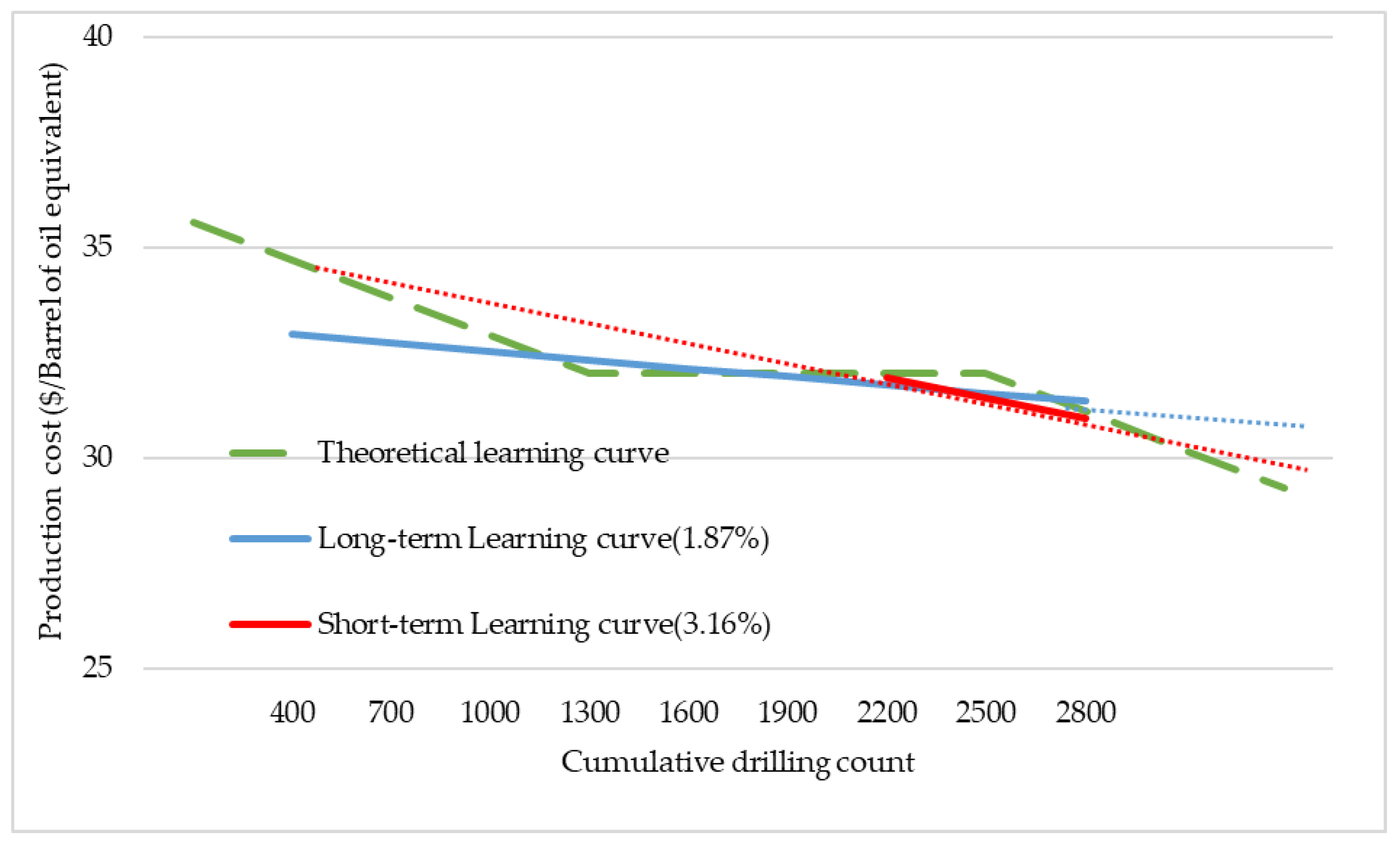
This discontinuous technological development (or decrease of production cost) contrasts with Fukui et al.’s [12] research results. Their research results use well-head price data to calculate learning rate, which could lead to overestimation since there is a gap between cost and price. The decline of natural gas and oil prices in the past two years were intended by OPEC, and did not result from technological developments [2]. This study uses cost data to reflect technological development and decrease of production cost. The use of cost data results in a discontinuous and step-wise-shaped production cost curve (as shown in Figure 2). Such discontinuous, step-wise technological development paths are consistent with previous studies. Arrow [20] describes this phenomenon as a steady phase and Schaeffer et al. [21] express it as a shake-out. With regards to the long-term learning curve, technological development of the shale E&P industry is interpreted as being stagnant. Technological development, according to the short-term learning curve, has resumed.
5. Conclusions
Unconventional petroleum production, consisting of shale gas and tight oil, has experienced fast growth since 2008. However, in 2014, crude oil and natural gas prices crashed due to OPEC’s squeezing strategy. Therefore, many shale E&P players faced a situation where they had to reduce their production costs to remain competitive. This study attempts to analyze production cost decrease from the past. To analyze the technological development trend, this study adopts the learning curve method by utilizing annual production cost and the drilling count data. The results of this study show two distinct learning curves estimated over two separate periods. The long-term and short-term model learning rates are 1.87% and 3.16%, respectively. This gap between the two models is a result of the decrease in production costs in 2016.
To summarize, between 2008 and 2011, the shale industry was able to improve productivity by developing a fracturing design and changing input choices [13]. From 2012 to 2014 there was a stagnant learning period. As a result, crude oil and natural gas prices were not low enough to motivate a reduction in production costs. However, after the fall of crude oil and natural gas prices, induced by OPEC’s squeezing strategy, technological development resulted in a production cost decrease in 2016.
This study attempts to measure the learning rate of US E&P players by using annual report data of companies. The results of this study show a low learning effect because learning works discontinuously. This research has an advantage in that it reproduces results of previous studies by analyzing production cost data.
Acknowledgments
This paper has been funded by National Research Foundation-2016R1A2B1014142 and National Research Foundation-NRF-2015-S1A3A-2046742 (SSK).
Author Contributions
Jong-Hyun Kim and Yong-Gil Lee conceived and designed the experiments; Jong-Hyun Kim and Yong-Gil Lee performed the experiments; Jong-Hyun Kim and Yong-Gil Lee analyzed the data; Jong-Hyun Kim and Yong-Gil Lee contributed reagents/materials/analysis tools; Jong-Hyun Kim and Yong-Gil Lee wrote the paper.
Conflicts of Interest
The authors declare no conflict of interest.
References
- Hartmann, B.; Sam, S. What Low Oil Prices Really Mean. Harv. Bus. Rev. Digit. Artic. 2016, 2–6, March 28. [Google Scholar]
- Behar, A.; Ritz, R.A. An Analysis of OPEC’s Strategic Actions, US Shale Growth and the 2014 Oil Price Crash; IMF Working Paper 16/131; International Monetary Fund: Washington, DC, USA, 2016.
- US Energy Information Administration (EIA). Annual Energy Outlook 2016 with Projection to 2040; US Energy Information Administration: Washington, DC, USA, 2016.
- Wright, T.P. Factors affecting the costs of airplanes. J. Aeronaut. Sci. 1936, 3, 122–128. [Google Scholar] [CrossRef]
- Buzzell, R.D.; Gale, B.T.; Sultan, R.M. Market share—A key to profitability. Harv. Bus. Rev. 1975, 53, 97–106. [Google Scholar]
- Day, G.S.; Montgomery, D.B. Diagnosing the experience curve. J. Mark. 1983, 47, 44–58. [Google Scholar] [CrossRef]
- Wene, C.O. Experience Curves for Energy Technology Policy; International Energy Agency (IEA): Paris, France, 2000. [Google Scholar]
- Oh, D.-H.; Lee, Y.-G. Productivity decomposition and economies of scale of Korean fossil-fuel power generation companies: 2001–2012. Energy 2016, 100, 1–9. [Google Scholar] [CrossRef]
- Hong, S.; Chung, Y.; Woo, C. Scenario analysis for estimating the learning rate of photovoltaic power generation based on learning curve theory in South Korea. Energy 2015, 79, 80–89. [Google Scholar] [CrossRef]
- Kahouli-Brahmi, S. Technological learning in energy-environment-economy modelling: A survey. Energy Policy 2008, 36, 138–162. [Google Scholar] [CrossRef]
- Lundvall, B.A.; Dosi, G.; Freeman, C.; Nelson, R.; Silverberg, G.; Soete, L. Innovation as an Interactive Process: From User-Producer Interaction to the National System Of Innovation, Technical Change and Economic Theory; Pinter: London, UK, 1988; pp. 349–369. [Google Scholar]
- Fukui, R.; Greenfield, C.; Pogue, K.; der Zwaan, B. Experience curve for natural gas production by hydraulic fracturing. Energy Policy 2017, 105, 263–268. [Google Scholar] [CrossRef]
- Covert, T.R. Experiential and Social Learning in Firms: The Case of Hydraulic Fracturing in the Bakken Shale; Harvard Environmental Economics Program: Cambridge, MA, USA, 2014. [Google Scholar]
- Middleton, R.S.; Gupta, R.; Hyman, J.D.; Viswanathan, H.S. The shale gas revolution: Barriers, sustainability, and emerging opportunities. Appl. Energy 2017, 199, 88–95. [Google Scholar] [CrossRef]
- Striolo, A.; Cole, D.R. Understanding Shale Gas: Recent Progress and Remaining Challenges. Energy Fuels 2017, 31, 10300–10310. [Google Scholar] [CrossRef]
- Chang, H.; You, F. Deciphering the true life cycle environmental impacts and costs of the mega-scale shale gas-to-olefins projects in the United States. Energy Environ. Sci. 2016, 9, 820–840. [Google Scholar]
- Weijermars, R. Shale gas technology innovation rate impact on economic Base Case—Scenario model benchmarks. Appl. Energy 2015, 139, 398–407. [Google Scholar] [CrossRef]
- Curtis, T. Unravellling the US Shale Productivity Gains; Oxford Institute for Energy Studies: Oxford, UK, 2016. [Google Scholar]
- Energy Information Administration (EIA). Trends in U.S. Oil and Natural Gas Upstream Costs; Energy Information Administration: Washington, DC, USA, 2016.
- Arrow, K.J. The Economic Implications of Learning by Doing. Rev. Econ. Stud. 1962, 29, 155–173. [Google Scholar] [CrossRef]
- Schaeffer, G.J.; Seebregts, A.J.; Beurskens, L.W.M.; Moor, H.H.C.; Alsema, E.A.; Sark, W.; Durstewicz, M.; Perrin, M.; Boulanger, P.; Laukamp, H.; et al. Learning from the Sun; Analysis of the Use of Experience Curves for Energy Policy Purposes-The Case of Photovoltaic Power; Final Report of the Photex Project, DEGO: ECN-C–04-035; Energy Research Centre of the Netherlands: Petten, The Netherlands, 2004. [Google Scholar]
Figure 1.
Annual production cost and cumulative drilling counts.
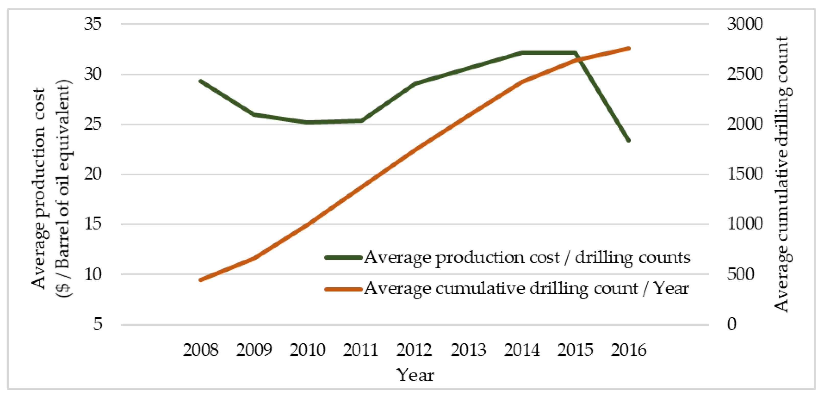
Figure 2.
Step-wise learning curve.


Table 1.
Variables of mathematical formula of the learning rate method.
| Wright’s Formula [4] | ||||||
| Variables | Y | X | n | |||
| mean | Production cost | Production quantity | Decline rate | |||
| Fukui’s Formula [12] | ||||||
| Variables | . | LR | ||||
| mean | Unit production cost | Unit production cost of first year | Cumulative drilling count | Cumulative drilling count of first year | Learning parameter | Learning rate |
Table 2.
Annual average production cost from 2008 to 2016. BOE = barrel of oil equivalent.
| Year | 2008 | 2009 | 2010 | 2011 | 2012 | 2013 | 2014 | 2015 | 2016 |
|---|---|---|---|---|---|---|---|---|---|
| $/BOE | 29.35 | 25.94 | 25.20 | 25.35 | 29.10 | 30.66 | 32.19 | 32.18 | 23.42 |
Table 3.
Regression model specification.
| Long-Term Regression Model (2008–2016) | Short-Term Regression Model (2014–2016) | |
|---|---|---|
| R2 | 0.096 | 0.098 |
| F | Less than 0.000 | 0.015 |
Table 4.
Results from learning curve calculations.
| Long-Term Learning Curve (2008–2016) | Short-Term Learning Curve (2014–2016) | |
|---|---|---|
| LR (Learning rate) | 1.87% | 3.16% |
| L (Learning parameter) | 0.0272 | 0.0464 |
| P(X0) (First year production cost) ($/BOE) | 32.93 | 31.92 |
| Required time approaching to double experience (year) | 3.05 | 2.02 |
© 2017 by the authors. Licensee MDPI, Basel, Switzerland. This article is an open access article distributed under the terms and conditions of the Creative Commons Attribution (CC BY) license (http://creativecommons.org/licenses/by/4.0/).
Share and Cite
MDPI and ACS Style
Kim, J.-H.; Lee, Y.-G. Analyzing the Learning Path of US Shale Players by Using the Learning Curve Method. Sustainability 2017, 9, 2232. https://doi.org/10.3390/su9122232
AMA Style
Kim J-H, Lee Y-G. Analyzing the Learning Path of US Shale Players by Using the Learning Curve Method. Sustainability. 2017; 9(12):2232. https://doi.org/10.3390/su9122232
Chicago/Turabian StyleKim, Jong-Hyun, and Yong-Gil Lee. 2017. "Analyzing the Learning Path of US Shale Players by Using the Learning Curve Method" Sustainability 9, no. 12: 2232. https://doi.org/10.3390/su9122232
Note that from the first issue of 2016, this journal uses article numbers instead of page numbers. See further details here.