Seasonal and Diurnal Characteristics of Land Surface Temperature and Major Explanatory Factors in Harris County, Texas


1
Department of Geosciences, Florida Atlantic University, Boca Raton, FL 33431, USA
2
Department of Geography, University of Victoria, Victoria, BC V8W 2Y2, Canada
3
Department of Atmospheric Science, The University of Alabama in Huntsville, Huntsville, AL 35805, USA
4
Department of Geography and Atmospheric Science, University of Kansas, Lawrence, KS 66045, USA
*
Author to whom correspondence should be addressed.
Sustainability 2017, 9(12), 2324; https://doi.org/10.3390/su9122324
Submission received: 25 October 2017
/
Revised: 11 December 2017
/
Accepted: 11 December 2017
/
Published: 13 December 2017
(This article belongs to the Special Issue Geospatial Technologies for Sustainable Natural Resources)
Abstract
:The effects of biophysical and meteorological factors on land surface temperature (LST) have been well studied in previous research. However, less attention has been paid to examine how building materials influence the magnitude of LST within an urban environment. This study investigates the interaction of biophysical and building wall materials to influence LST in Harris County, Texas, USA using multiple stepwise linear regression analyses and neighborhood analysis. Working at 1 km grid resolution, LST data is related to impervious surface fraction, albedo, distance to water bodies, and seven major wall types. Ten years of aggregated MODIS (Moderate Resolution Imaging Spectroradiometer) daily LST products were used to calculate the mean LST in January and August for daytime and nighttime conditions. Harris County 2010 parcel level building property data were used to create composition characteristics of the building wall types. Our results demonstrate that both biophysical and building wall characteristics significantly influence the spatiotemporal variations of LST. However, biophysical factors are the dominant explaining factors compared to building wall materials. Impervious surface fraction is the most significant variable to explain the variation of LST, and has positive effects on LST. In contrast, high albedo materials and the presence of open water bodies significantly affect LST and are good candidate variables to mitigate the heat island effect. Furthermore, the building wall variables all increase LST for both daytime and nighttime, but different wall materials have various effects on LST. Brick/veneer and frame/concrete block are the two dominant wall types in Harris County and tend to generate higher LST. These results demonstrate how building materials, in combination with biophysical factors, can be used to mitigate neighborhood-scale LST. This methodology works reasonably well for Houston, but is likely to be more effective in higher density urban settings.
1. Introduction
Urbanization represents the most dramatic human alteration of the land surface, typically resulting in the formation of urban heat islands (UHI) [1]. UHI refers to the higher atmospheric and surface temperature in urban areas compared to surrounding areas with more vegetation. The primary cause is the loss of latent heat and a resulting increase in sensible heat exchange in sparsely vegetated urban settings with a greater number of impervious surfaces and the nature of the urban fabric in part determined by road, wall, and roof materials [2]. As a consequence, water consumption and energy use typically increase in warmer urban areas because of increased temperature and moisture stress. Generally, there are two categories of UHI: atmospheric UHI and surface UHI (SUHI) [3]. They are based on how temperature is measured, e.g., air temperature versus land surface temperature (LST). Traditionally, researchers studied the UHI phenomena using air temperature data measured by thermometers at weather stations or on automobiles [4,5,6]. Rao [7] first raised the possibility of identifying the thermal signature of urban regions through satellite images, which can easily provide both the magnitude and spatial distribution of LST [8,9]. With the advancement of remote sensing technology, a wide range of moderate and high spatial resolution thermal infrared images have been employed to study UHI and LST, such as Landsat ETM+ (Enhanced Thematic Mapper+) with 30 m resolution, ASTER (Advanced Spaceborne Thermal Emission and Reflection Radiometer) with 90 m resolution, and MODIS (Moderate Resolution Imaging Spectroradiometer) with 1 km resolution [10,11,12,13,14,15,16,17,18,19,20].
The general spatial distribution and variation of LST over urban areas have been well documented in literature, and significant factors explaining the spatial variations have been identified. For example, Xiao et al. [14] found that LST values increased from the outskirts towards the inner urban areas in Beijing, China, with temperatures ranging from 16.4 °C to 40.5 °C on 31 August 2001. Remotely sensed LST records the radiative energy emitted from the surface, including building roofs and walls, parking lots, water bodies, vegetation, and bare ground [3]. As a result, there is a close relationship between physical characteristics of various urban surfaces and the LST in urban environments; typically resulting in a mosaic of temperature patches across the urban space [21]. Previous research has shown that there is a significant statistical relationship between LST and biophysical factors [11,13,14,22]. For example, Weng et al. [22] demonstrated that the unmixed vegetation fraction in a grid cell, representing an indicator of vegetation abundance, has a strong negative correlation with LST. Yuan et al. [11] found there is a strong linear relationship between LST and the percentage of impervious surface areas. Morabito et al. [23] used 5-m resolution imagery and converted the imperviousness degree into a binary product using a threshold (0–29% is non-built-up surface and 30–100% is built-up surface) for four cities in Italy. They used MODIS products (2001–2013) to extract the LST. Then they analyzed the relationships between LST values and built-up surfaces through a linear regression analysis, and the results demonstrated that the built-up surfaces explained around 60% of LST variation and concluded that impervious surface fraction is the major driver of surface urban heat. Other non-biophysical factors are also considered in some research, such as land use/land cover (LULC) configuration and pattern [20,24,25,26,27], LULC change [28,29], socioeconomic factors [14,30], and topographic factors [8]. Among all these factors studies, biophysical factors are most important to explain LST variation [13]. While many studies have looked at the impact of urban morphology on UHIs, observations of urban fabric properties on UHIs has not been well documented. The aim of this study is to determine to what extent building materials affect the UHI.
Earlier satellite based studies of UHIs focused on the phenomena during daytime in summer because more images are available with high and moderate resolution during the daytime than nighttime [15,31]. However, UHIs develop mainly at night throughout the year and heavily depend on weather conditions [3]. Moreover, the nocturnal SUHI has different characteristics and causes compared to daytime SUHI development. Kardinal Jusuf et al. [32] observed that surface temperatures associated with different land use types were dissimilar during daytime and nighttime based on the qualitative and quantitative analysis. Buyantuyev et al. [33] found that while vegetation was the most significant determinant of daytime LSTs, pavements explained spatiotemporal variation of LST during nighttime the most. Seasonal changes also affect the energy balance of ecosystems on the earth [33], and the intensity of UHI in arid and semi-arid environments has large seasonal variability because of the vegetation phenology [34]. As a result, the comprehensive diurnal and seasonal LST variations and the corresponding explanatory factors should be fully studied. Previous research has concentrated primarily on biophysical and meteorological factors determining LST in the urban environments. Building envelopes are known to be a dominant factor in the energy consumption of buildings [35], thus it is likely that wall and roof types with different thermal behaviors will also impact outdoor thermal environments. While the effects of building morphology have been studied with respect to ventilation and UHI development, there has been almost no research on how building wall characteristics influence LST intensity within a big city. The aim of this study is to specifically evaluate how the urban fabric impacts daytime and nighttime UHI characteristics in both summer and winter.
This study focuses on the Harris County, Texas. Harris County has experienced a mean UHI growth of 0.8 K from 1985–1987 to 1999–2001 [36]. This increase is attributed to a lack of appropriate planning strategies and accelerated urban development. Previous studies of UHI and LST in Harris County have concentrated on assessing its magnitude and causes [36,37], but these studies do not consider building wall properties as a potential source of UHI variability in Houston. This study investigates the seasonal and diurnal distribution and causes of variability of LST within Harris County using RS, GIS and statistical analyses. The specific objectives of this study are: (1) to investigate the urban–rural and intra-urban variability of LST seasonally and diurnally in Harris County; (2) to examine the quantitative relationships between LST variations related to known biophysical variables that affect UHI intensity including impervious surface fraction (ISF), albedo, distance to water bodies (used as control variables) and, to investigate the effect of building materials on UHI; and (3) to compare neighborhood scale thermal responses to different building wall types through a neighborhood analysis. The results from this research will enhance our understanding of the seasonal and diurnal variations of LST. In addition, this analysis aims to explain how building wall types can explain local variations of LST. Finally, the results would provide useful information and important insights to urban planners and natural resource managers attempting to effectively mitigate the UHI effects through urban design and selection of a particular wall type in order to improve the thermal environment in big cities, such as Houston.
2. Data and Methodology
2.1. Study Area
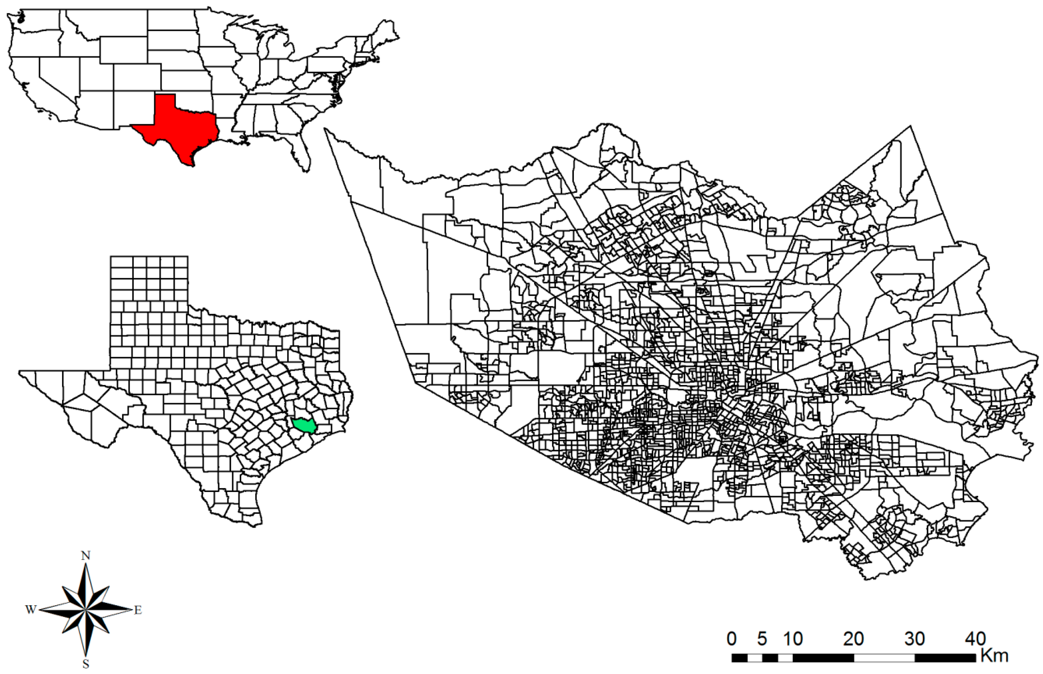
Harris County, the largest county in Texas and the third largest in the USA, is selected as a case study for this research (Figure 1). Containing Houston, the largest city in Texas and the fourth largest populous city in the U.S. (2010 U.S. Census), Harris County has a population of over 4.1 million within a land area of 4478 km2. A humid, subtropical climate characterizes the county, which experiences hot, humid summers and generally mild to cool winters, and an average yearly precipitation of 1200 mm. Land cover features are typical of those in urban and suburban environments, including urban and built-up areas, cropland/natural vegetation mosaics, woody savannas, croplands, grasslands, mixed forests, sea and land water bodies [38]. The lack of striking topography in Harris County is advantageous to study the variation of LST. Two nearby large water bodies in Harris County are Galveston Bay to the east of the county, and the Gulf of Mexico is approximately 80 km to the south-east [37]. These features influence the local climate and thermal environment of Harris County [39,40].
2.2. Datasets and Image Processing
Five primary data sources are employed in this research: (a) the 2010 building property data were obtained from the parcel dataset to capture the composition characteristics of building wall types; (b) MODIS version 5 land cover type products (MCD12Q1, 500 m, yearly) for 2010; (c) MODIS version 5 daily LST/emissivity products from 5 March 2000 (MOD11A1), 8 July 2002 (MYD11A1) to 31 December 2010 with 1 km spatial resolution; (d) ISF data is from the National Center for Atmospheric Research (NCAR) Weather Research and Forecasting (WRF) dataset [41] at the same 1 km grid resolution; (e) MODIS version 5 16-day composited albedo products (MCD43A3) with 500 m spatial resolution for the year of 2010. MODIS albedo products provide white sky albedos (WSA) and black sky albedos (BSA). In this research, we only use WSA over shortwave broadband (0.3–5.0 µm), because BSA is linear with WSA and shows similar results to WSA [42].
MODIS is a 36-band instrument aboard the Terra and Aqua satellites, which covers the earth surface four times each day: during the daytime at about 10:30 a.m. and 13:30 p.m. local solar time and during the nighttime at about 22:30 p.m. and 1:30 a.m. local solar time. The MOD11A1/MYD11A1 products are produced daily through the generalized split-window LST algorithm [43]. After reprojection and resampling the data were projected into WGS84 spatial reference system. We also masked the cloud-contaminated pixels (with extremely low LST values) in the processing considering both the location and climate in Harris County, see [38] for more details. To overcome missing data due to the presence of clouds, the LST was temporally aggregated [38]. To create an average daytime and nighttime LST dataset, the Aqua daytime (13:30 p.m. local time) and Terra nighttime (22:30 p.m. local time) were averaged from 2000 to 2010 for each month. The monthly mean of LST was used as the independent variable in later statistical analyses. The land cover data and albedo data were projected to the same coordinate system as the LST data, and were resampled to 1 km spatial resolution using the majority and cubic convolution resampling methods, respectively.
2.3. Extraction of Building Wall Types
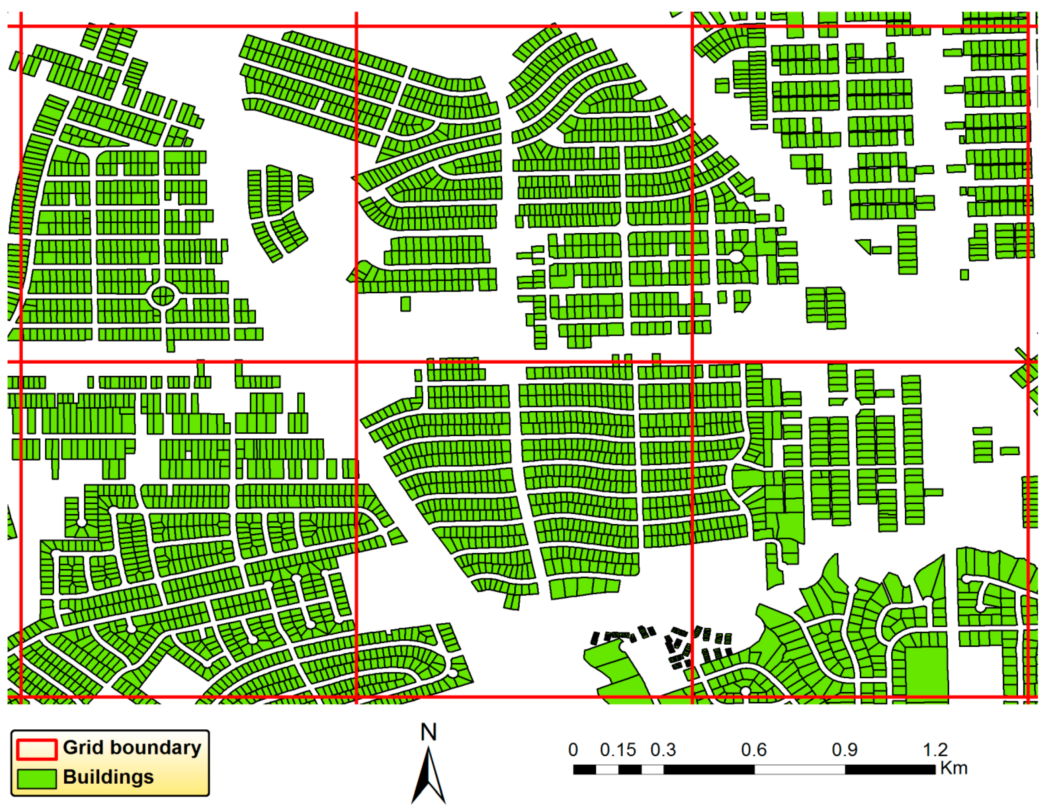
The building parcel data of Harris County in 2010 are in vector format, and building wall types were aggregated from the parcel level to a 1 km × 1 km grid (Figure 2) consistent with LST and biophysical factors. Parcel data consist of 1,047,768 records of residential buildings and 187,910 records of commercial buildings in Harris County. The building parcel dataset contains a number of variables regarding conditions and materials of buildings and a number of variables are aggregated, and we used the building wall types to characterize the housing makeup of each grid cell. There are 15 building wall types in total for residential buildings and commercial buildings in this dataset, which are aluminum/vinyl, asbestos, brick/masonry, brick/veneer, fireproofed steel, frame/concrete block, masonry bearing, mobile home, open steel skeleton, reinforced concrete, residential, shake shingle, stone, stucco, and wood frame. However, some wall types do not appear very often in Harris County based on a simple descriptive statistical analysis, so we chose the seven most prevalent building wall types as the explanatory variables in the following statistical analysis, which are brick/masonry, brick/veneer, frame/concrete block, masonry bearing, open steel skeleton, stucco, and wood frame. The 1 km × 1 km grid and building parcel dataset (Figure 2) were overlain. In the spatial overlay process, some large buildings occupy two or more grids. In order to simplify the analyses, such building types were assigned to the grid cell associated with the parcel’s centroid location. Then percentages for seven major building wall types were calculated based on the following procedures in each grid.
The building parcel dataset provides the number of buildings in each parcel and their corresponding wall types. Assuming the buildings located in a grid (1 km × 1 km) are clustered and they have similar height, width, and other morphological characteristics, then we estimated the percentage of each building wall type within each grid as follows:
where is the percentage of stucco wall type in a grid, is the number of parcels in a grid containing the stucco wall type, is the number of buildings with stucco wall type in the jth parcel, is the total number of parcels within a grid, and is the total number of buildings in the ith parcel. The percentage of the other six wall types is calculated in the same way.
2.4. Computation of Distance to Water Bodies (Dist2Water)
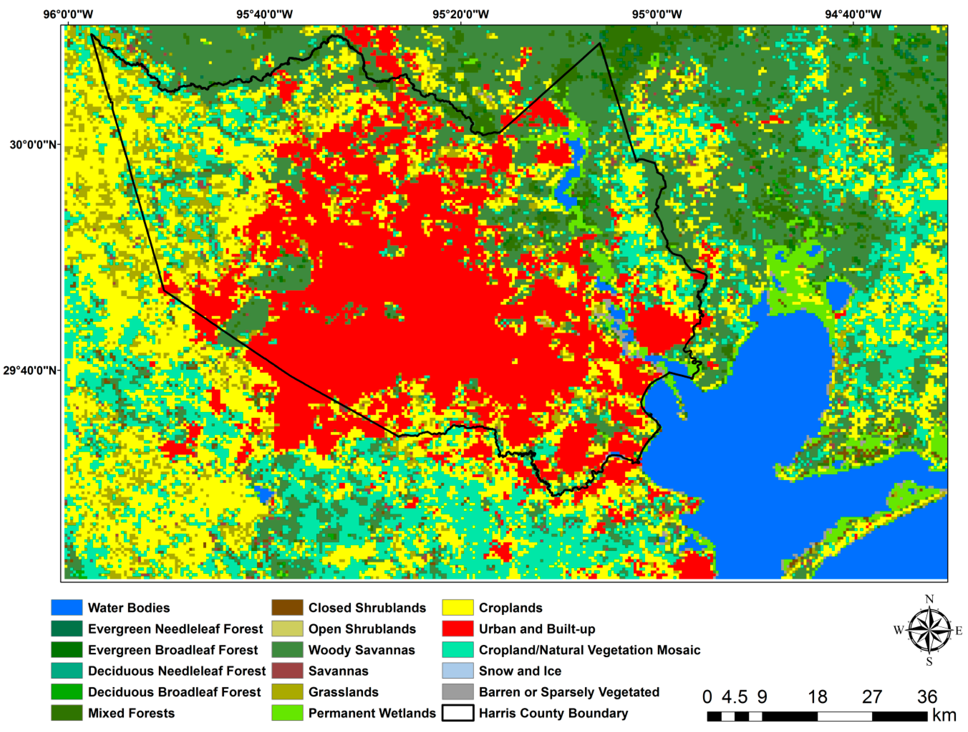
Harris County is adjacent to Galveston Bay and other water bodies, which greatly affect local climate and thermal environments. Thus, the proximity to a water body is expected to influence LST values within a grid cell. The Dist2Water variable is based on the Euclidean distance between a land grid cell and the nearest grid covered by water. The 2010 MODIS land cover type product (MCD12Q1, Figure 3) is used to identify water and non-water grids. We choose the International Geosphere Biosphere Program (IGBP) classification schemes to classify land cover types. This scheme includes 17 classes with natural vegetation, urban and built-up, and non-vegetated land classes.
2.5. Statistical Analyses
In order to examine the relationship among spatial variations of LST, biophysical factors and building wall characteristics, the following explanatory variables were selected: ISF, white sky albedo, Dist2Water, and percentage values of the seven major building wall types in each 1 km × 1 km grid cell containing buildings. A multiple stepwise regression was performed to identify independent variables with statistical significance (p < 0.001) for predicting variations in LST. It is implicit in this analysis that the biophysical factors have been demonstrated to be important to determine the UHI intensity [13,14,42], and thus we used these variables to control the effects of building density, vegetation fraction, and the influence of nearby water bodies on the UHI. The wall type variables were used to estimate the impact of building wall types on the local UHI variability. The variables removed from the multiple stepwise regressions are not considered as significant explanatory factors. Four regression models were built to predict variation in mean daytime and nighttime LST for January (representative of winter) and for August (representative of summer) for the period 2000–2010. In these four models, only white sky albedo changes significantly in the two months, other independent variables were constant.
2.6. Neighborhood Analysis
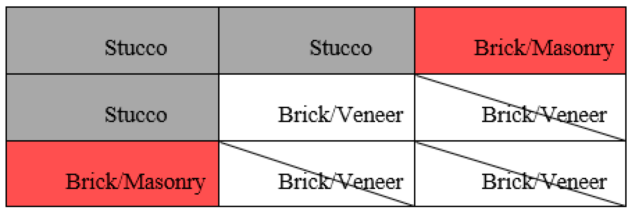
A second approach to determine the potential effects of wall types on LST using a 3 × 3 neighborhood analysis was performed to compare LST differences between neighboring grids with different dominant wall types. The dominant wall type was extracted for each grid and grids were only included in the analysis if the dominant wall type represents more than 40% of all building types. In addition, the grids entered into the analyses were required to have ISF values above 0.5 to isolate high density urban grid cells with relatively homogenous housing and biophysical characteristics. Figure 4 is an example to illustrate how the 3 × 3 neighborhood analysis is implemented. In this example, a centered grid with brick/veneer as its dominant wall type (>40%) and more than 0.5 ISF is compared to its eight neighboring grids. The surrounding grids are checked to see if they have a different dominant wall type as well as meeting the minimal ISF and dominant wall type criteria. If the cells meet the criteria, the LST difference between the centered grid and the surrounding grid was calculated. If the surrounding grids have the same dominant wall type as the centered grid or otherwise did not meet the minimum criteria, they were discarded from the analysis. The LST difference between each possible combination of two different wall types resulted in a total of 21 comparisons among those seven building walls.
3. Results
3.1. Seasonal and Diurnal Characteristics of LST Variations
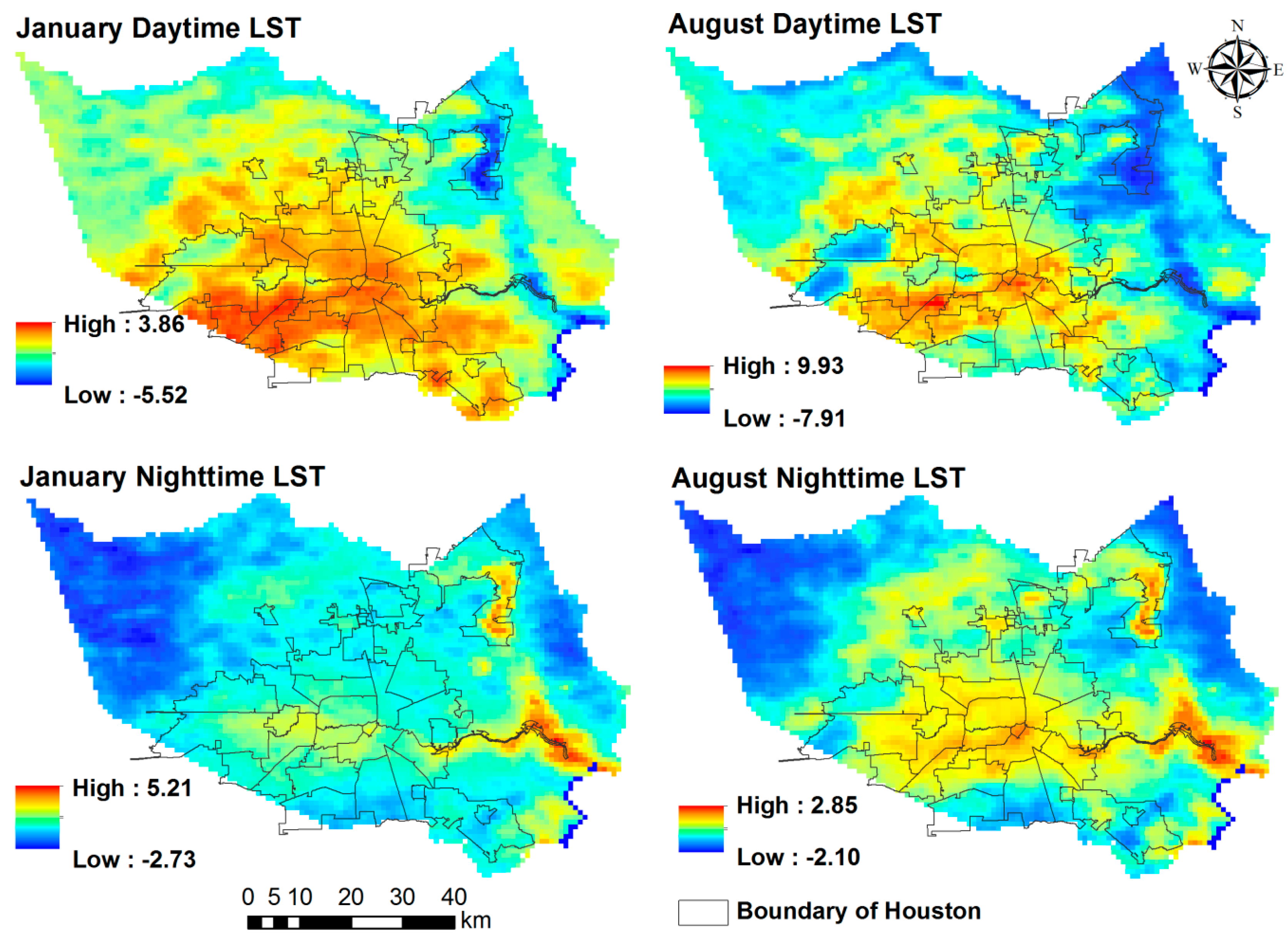
In order to analyze seasonal and diurnal characteristics of LST variations, we calculated the mean LST for daytime and nighttime in January and August from 2000 to 2010, respectively. To better compare the magnitude, spatial pattern and variation in LST maps (Figure 5), the spatially averaged LST was subtracted from the original LST values. Although the two seasons have different LST means and ranges, our analysis focuses on the spatial pattern and variations of LST. Generally, both daytime and nighttime LST values increased from the countryside towards the central business districts of the City of Houston. Both daytime and nighttime LST spatial variations for January and August were quite similar. The spatial distribution of LST is closely linked with the land cover distribution (Figure 3, [44]).
For the daytime LST maps, a number of hot spots can be identified in urban areas. These maps have high temperature zones clustered towards the central, northeast and southwest districts of city of Houston, which is consistent with the distribution of urban and built-up areas with higher impervious surface fractions (Figure 6) including industrial buildings, residential buildings, parking lots, gardens, asphalt on roofs, and other types of impervious surfaces. Without water sources for evapotranspiration, higher surface temperatures resulted in larger temperature gradients to drive sensible heat fluxes. Low temperature zones are clustered in the regions covered by water bodies, and in the northwest district covered by wooded wetlands with lower impervious surface fractions and near water sources which increase latent heat fluxes (Figure 6). In addition, the land surface energy balance includes the anthropogenic fluxes, such as the emissions from use of automobiles, air-conditioners, combustion engines, and other electrical equipment which can be turned into sensible or latent heat fluxes, and surface heat storage [42]. Although most rural areas experience lower LST compared to urban areas, there are still some hot spots where land cover includes dry land vegetation, and croplands.
Nighttime LST maps show that the highest temperatures are in areas covered by water bodies and wetlands. Water bodies have higher thermal inertia to slow down heat transfer at night. Built-up areas are clustered as high temperature areas. The low temperature areas are clustered towards the south and southeast districts with low-density built-up areas. Most of the rural areas are cold spots because of large amounts of vegetation and less anthropogenic heat.
Comparing daytime and nighttime LST shows that the diurnal temperature range is reduced in the central urban and high-intensity building areas, while croplands/natural vegetation areas with less human activity experience a greater diurnal temperature range which also has been documented in other studies [13,45]. Water bodies and wetlands have the lowest daily temperature range because water allows light to penetrate into deep layers without sensible heat transfer during the day resulting in cooler surface temperatures, while at night water bodies lose heat less slowly compared to land to form a hotter surface. Roth et al. [44] studied three coastal cities including Vancouver, Seattle, and Los Angeles, and also reported a similar discovery.
3.2. LST Relationship with ISF, Albedo, and Dist2Water
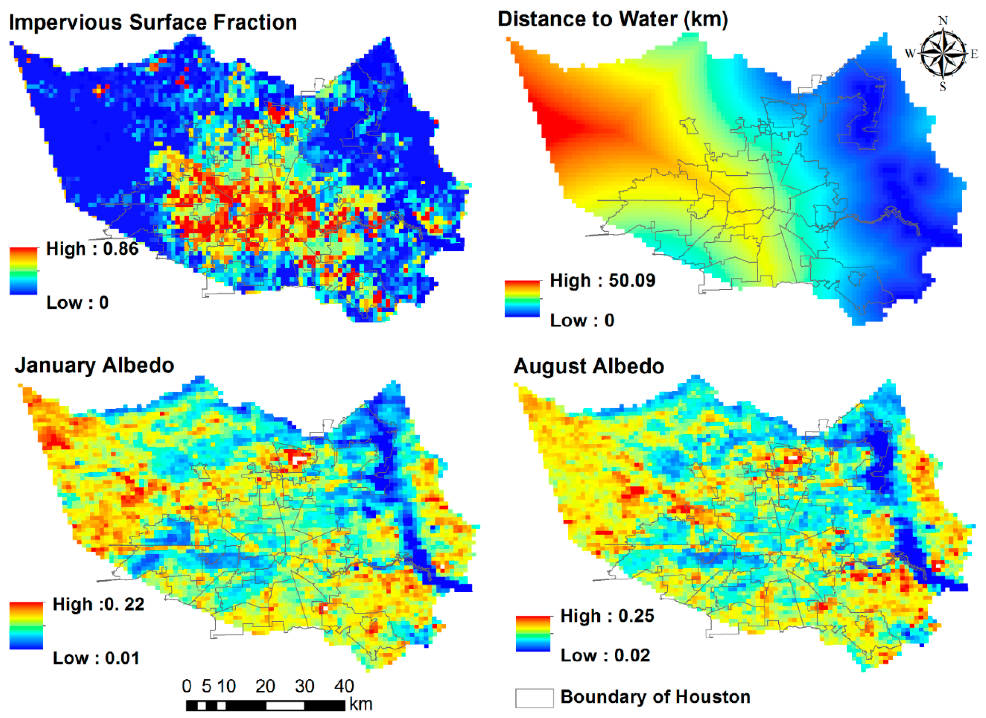
Four stepwise regression models were built, one for each daytime and nighttime scene in January and August (Table 1). Each model explained about the half of LST variations (R2 is approximately 0.5). In all cases the parameter entering the model first, and explaining most of the variance is ISF, a control variable for the purpose of this study. Dist2Water, also a control variable, an indicator for water availability in the local environment, is the second variable in the August daytime and January nighttime models, while albedo (also control) is the second entry variable in the August nighttime and January daytime variables. The August nighttime and January daytime models also both share albedo as the third entry variable. However, the third entry variable for the other two models (January daytime and August nighttime) is brick/veneer wall followed by Dist2Water in both these models. Brick/veneer wall is also the fourth entry variable in the August daytime and January nighttime models. After these variables, different wall types are the remaining significant variables entering the equations, generally going from heavier weight wall types to lighter weight walls in succession. In all models, ISF, albedo, and Dist2Water are all significant at the 0.001 confidence level. Furthermore, these three independent variables accounted for approximately 90% of the total variation of LST explained in each model. Model coefficients for ISF are all positive indicating that higher ISF values increase LSTs regardless of season or time of day [8,11,20,46]. During daytime, the heat fluxes primarily come from regions with higher ISF that more easily absorb solar radiation. This is due to the fact that there is little water available on these surfaces for latent heat loss, and because higher ISF generally means a lower vegetation fraction within the grid cell. At nighttime, the heat mainly comes from the energy stored during the daytime and anthropogenic activities, such as transportation and manufacturing, which are highly correlated with ISF (Figure 6).
Surface heat storage, both in natural bodies and buildings, has a very close relationship with solar energy absorption (albedo) and thermal properties (heat capacity and thermal conductivity) of surface materials [42,47]. This relationship is reflected in the coefficients for albedo and Dist2Water that are negative at night and positive during the day. This suggests that increases in these values increase temperatures during the day both as distance from a water body increases, and as grid cell albedo values increase, and vice versa at night in both seasons. While this relationship is very intuitive for water bodies that have high heat capacity reducing diurnal temperature ranges relative to the surrounding landscapes, the relationship with albedo is counter-intuitive. High albedo should reduce energy absorption during the day and lead to cooler values for buildings, and lower heat absorption during the day due to albedo should reduce energy availability at night and be demonstrated at the building level [48]. However, a comparison of the LULC (Figure 3) and albedo (Figure 6) shows that areas with low albedo are most closely linked to water bodies, grasslands, wetlands, and also developed regions with significant asphalt areas, and high albedo materials are mainly found in rural areas with dry soil and developed regions such as concrete surfaces. This implies that the albedo–LST relationship is complicated in part because both low and high albedo areas can have either reduced or enhanced LST values. But the large extent of the low albedo vegetated areas relative to the built up areas dominate the signal resulting in a similar relationship to the Dist2Water variable. Giridharan et al. [48] also reported the heat island intensity had a positive relationship with surface albedo in the daytime, but had a negative relationship at nighttime in the late summer, when using Hong Kong as the study area.
3.3. The Relationship between LST and Building Wall Types
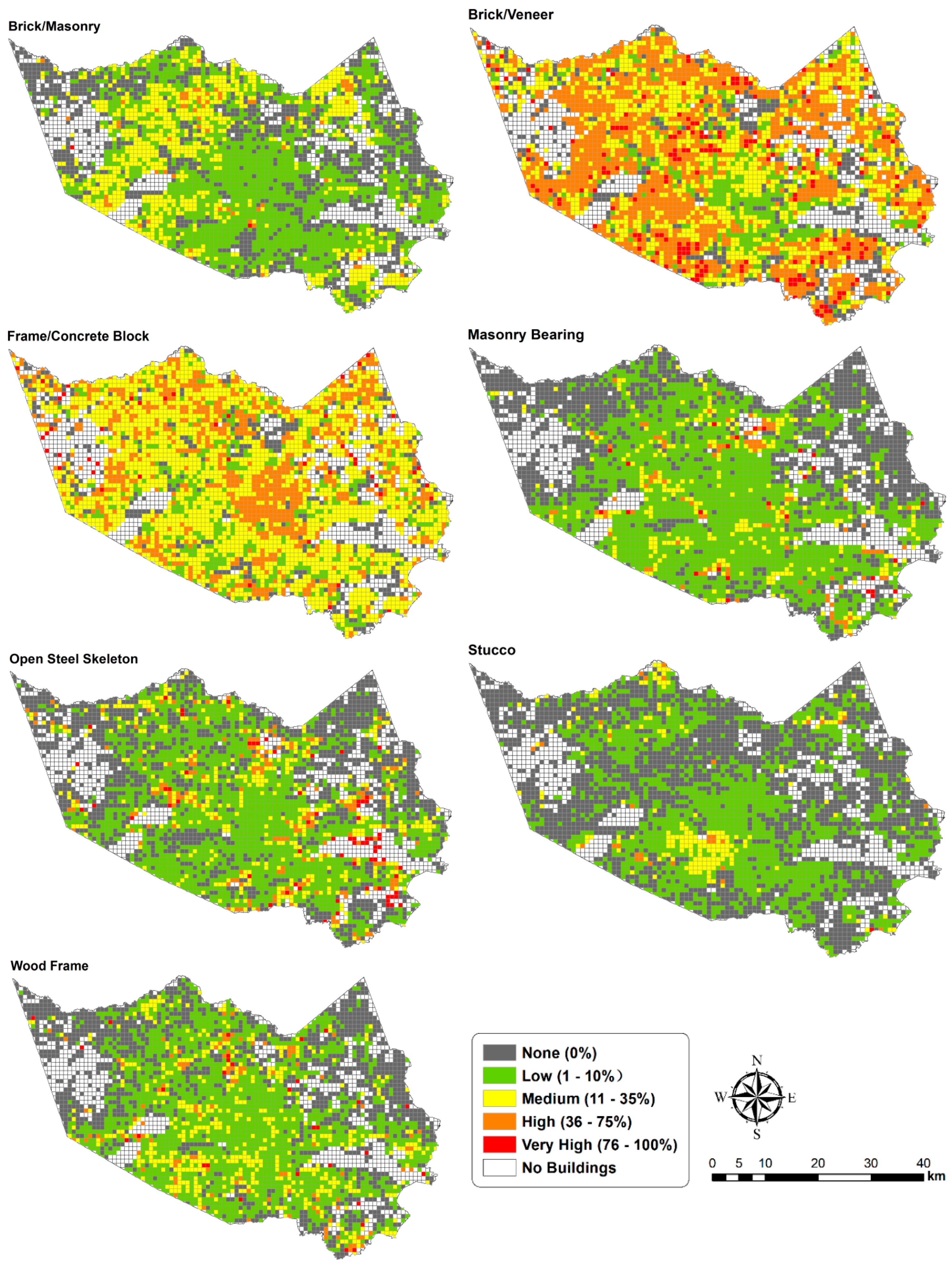
Seven major building wall variables are also selected as explanatory variables in the stepwise regression models. In the August (summer) nighttime model (Table 1; Model 4), the seven building wall variables all enter into the stepwise regression model, but building wall variables do not enter into the other three models completely. Generally, brick/veneer, frame/concrete Block, open steel skeleton, and wood frame are much more significant explanatory variables than the other building wall variables across all models; not only with respect to their presence, but also with their order of entry (Table 1). These four wall types are also the most popular wall types in Harris County (Figure 7) making their relationships more significant compared to the remaining low occurrence wall types. Brick/veneer is the most important building wall variable, which is always the first building wall variable entering the four models, and is more important than Dist2Water in Model 1 (January daytime) and Model 4 (August nighttime). In all four models the building wall variables significantly add to the explanation of LST variations. Furthermore, except for the open steel skeleton and stucco wall types in Model 1 (January day), all wall variables are significant at the 0.001 confidence level in all cases. Overall building wall variables explained 4.7% out of 41.2% total explained variance for Model 1 (January day), 5.5% out of 55.2% total explained variance for Model 2 (January night), 4.8% out of 45.3% explained variance in Model 3 (August day) and 7.2% out of 47.2% total explained variance for Model 4 (August night). These results show that wall types have a stronger predictive power in the nighttime models of the total variation of LST, and demonstrate that these variables are much weaker at explaining the variation of LST compared to ISF, Dist2Water, and albedo in general. The building wall variables all have a positive correlation with LST variation in the four models, suggesting that LST increases with the percentage increase of the building wall variables including both daytime and nighttime in different seasons. A higher percentage of building walls means that there are more residential or commercial buildings producing anthropogenic heat from air conditioning, refrigerators, and so on during the day and night. A large number of buildings also implies less vegetation, and possibly higher levels of human activities. These factors all contribute significantly to the increase of LST, no matter whether it is daytime or nighttime in different seasons.
3.4. Neighborhood Analysis
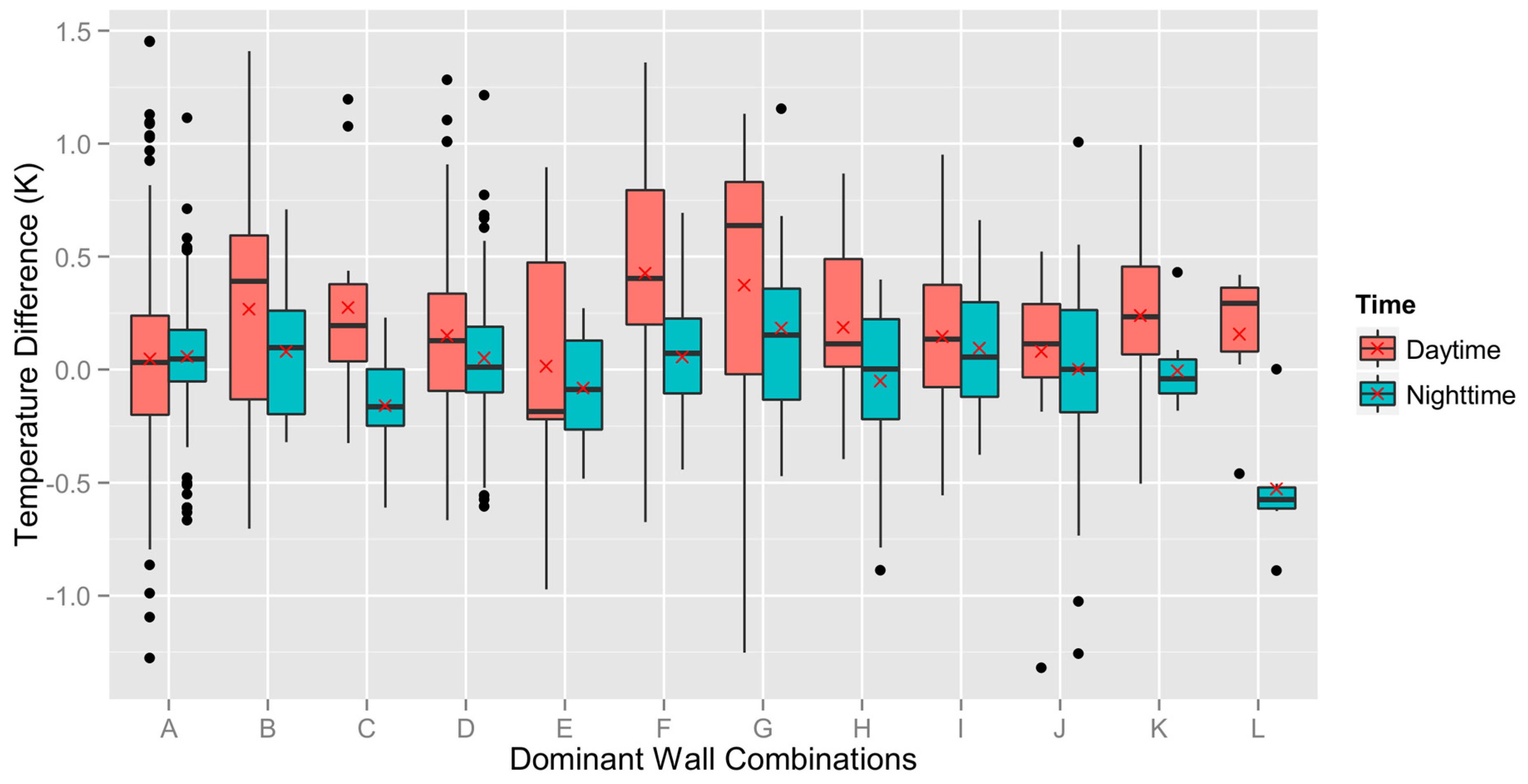
The daytime and nighttime LST differences between proximate grid cells with different building types is calculated using the neighborhood analysis, and we combined the January and August LST fields to increase the number of comparisons among different wall types. After the initial neighborhood analysis, the LST difference between two types of building walls is kept only when there are at least 50 pairs of comparisons in order to ensure enough samples for the following statistical analysis. Although there should be 21 combinations among seven building walls, 12 different combinations (Figure 8) of building walls met the requirements of percentage of dominant wall type, ISF, and sample size. First, to evaluate the statistically significant difference for LST among these wall types, a t-test is performed, and the differences are statistically significant with a p < 0.05 except E combination during daytime and J combination during nighttime. The boxplots in Figure 8 demonstrate that the mean LST difference for different neighboring walls is not large, with a maximum value of 0.4 K (F combination during daytime). The daytime LST difference is always greater than the nighttime LST difference. C, E, H, K, L combinations have different signs between daytime and nighttime averaged LST difference, but the other seven combinations have the same sign for daytime and nighttime average LST differences. Among the 12 combinations, only brick/veneer is compared with the other six wall types directly, because there are 1733 grids where brick/veneer is dominant. The three other most popular wall types are frame/concrete block (830 grids), wood frame (325 grids), and open steel skeleton (310 grids). There are about 50 grids with brick/masonry, masonry bearing, or stucco as dominant wall respectively. As a consequence, we focused on LST differences for brick/veneer, wood frame, frame/concrete block, and open steel skeleton. Based on the results of neighborhood analysis for both daytime and nighttime observations, the wall rankings associated with the highest LST magnitudes are brick/veneer, wood frame, frame/concrete block, and open steel skeleton. These results further support the conclusions from the regression analysis.
4. Discussion
Our results in this study reveal that both biophysical factors and building material properties (focused on building wall characteristics) influence the magnitude of urban LSTs. The quantitative relationships found in this study demonstrate that building wall type (representing different energy absorption, heat capacities, and conductivities) influences urban LSTs much like natural land cover types. By improving this understanding, these results can provide a series of useful strategies to mitigate the urban heat island and its adverse effects.
4.1. The Influence of Biophysical and Morphological Building Factors on LST
In this research, three biophysical factors and seven building wall variables are considered to explain the variation of LST at daytime and nighttime in the summer and winter. The stepwise regression analyses indicate that ISF, albedo, and Dist2Water play the dominant role in explaining the spatiotemporal variation of LST in Harris County. The combination of biophysical factors and building wall variables only explains approximately half of the variance of LST in the four models, which is lower than many previous studies reported [11,14]. These previous studies demonstrated that a strong linear correlation existed between ISF and LST at the regional scale. For example, Li et al. [46] demonstrated that the correlation coefficient between ISF and LST was around 0.9 in spring and summer at the regional level. In our research, although the ISF is the most significant explaining variable among the ten variables, it does not have very strong relationship with LST (R2: 0.204–0.340). These results are mainly because of a scale issue. Generally, a coarser scale could generate a much stronger correlation, i.e., the relationship between biophysical factors and LST is complicated based on the grid-by-grid analysis. At a finer scale, more detailed variables should be taken into consideration [20], such as the distribution of urban buildings, surface roughness, elevation, and so on.
During the daytime, the main heat source is solar radiation. However, nighttime heat sources mainly come from the heat accumulated during daytime, and anthropogenic heat emission from the city. This observation could be verified by the diurnal and seasonal analyses of LST variations, and the quantitative relationships between LST and its major drivers. For example, LST is always positively related to ISF and building wall variables, but negatively related to albedo and Dist2Water at night. Urban areas generally have higher LST and lower albedo compared to rural areas. As a result, these urban surfaces absorb more solar radiation during the daytime and emit heat as long wave radiation at nighttime. Furthermore, anthropogenic activities mainly happen in the urban areas with high electricity use and energy consumption. In this study area, the presence of open water bodies is an important cooling factor during the daytime, and a heating factor during nighttime because of thermal inertia.
As for building wall variables, their thermal storage ability is related to thermal conductivity and the specific heat capacity of wall materials. For example, brick, masonry, and concrete have much higher thermal conductivity and heat capacity compared to wood. Building walls that have higher thermal conductivity and heat capacity are able to absorb more energy during daytime and they take longer to release energy at nighttime. In the regression models, brick/veneer and frame/concrete block both have more important positive effects on LST responses compared to other wall types because of these property differences. In the neighborhood analysis, the grids with brick/veneer as the dominant wall type also have the highest observed LSTs. Although we ranked the LST magnitude, the LST differences among the 3 × 3 neighborhood are not very large (0.01–0.4 K). Other building morphologies possibly play a key role in determining an overall LST outcome, such as the sky view factor, and neighborhood height/width ratios.
4.2. Implications for Urban Planning and Management
The results that the biophysical and building wall variables influence variation of LST can provide insight for useful strategies and implications on how to counteract and mitigate urban heat islands. Impervious surfaces have little vegetation, and ISF is the major driver of urban heat. Although we cannot remove all of the pavement and other impervious surfaces and keep cities functional, more vegetation, especially a tree canopy, can be planted in appropriate locations. Surface albedo is another important factor. In order to decrease the heat stored in different surfaces at daytime, we could increase the amount of high albedo surfaces, such as white roofs and walls [49]. Rosenfeld et al. [49] demonstrated that a single building could generate 20–40% energy savings with a higher albedo. Water bodies are also a useful mechanism to mitigate urban heat, so buildings could be built closer to water bodies in order to decrease the use of energy for cooling in the summer. As for building wall materials, although brick, concrete, and masonry have higher thermal masses and probably cause higher LST, the appropriate use of these materials could provide a much more comfortable indoor environment so that the energy consumed for heating and cooling could be optimized and reduced. As a consequence, this research provides building designers some useful knowledge on how to design more environmentally friendly and efficient building walls with different layers and materials.
4.3. Limitations
This research also has some limitations. First, a single impervious surface fraction data was used in different seasons in this research. Previous research has shown that impervious surfaces are often considered as pseudo-invariant parameters [50] because of the insensitivity of spectral features to seasonal changes [46]. However, Li et al. [46] reported that there are variations of ISF between the early spring and the summer TM (Thematic Mapper) images. Therefore, further studies should explore the variation in ISF across different seasons. Second, ten years of aggregated MODIS daily LST products with 1 km spatial resolution were used in this study. However, other higher resolution thermal infrared images could be explored to improve the fine scale analyses, such as Landsat 8 TIR band data (30 m) [51] and ASTER images (90 m) used for retrieval of LST [52]. Third, building wall materials should directly affect the air temperature, so these building wall variables in this research should be much more important and obvious when we study the air temperature heat island. However, the observations of air temperature do not have the same spatial resolution as surface temperature. In a future study, modeling of air temperature could be used to further explore the relationship between LST and the building wall types. Finally, roof surfaces should have a more direct relationship with LST than the wall surface. However, we could not get accurate roof surface data for this current study. This kind of data should be used in the future in order to better predict the variations of LST.
5. Conclusions
The most dramatic anthropogenic LULC modification of natural environment is arguably urban development, generating urban heat islands. This research investigated the relationship of LST with both biophysical and building wall materials for daytime and nighttime conditions in the summer and winter. The results demonstrate that both biophysical and building wall factors influence the spatiotemporal variations of LST. However, the biophysical factors are the dominant explanatory factors compared to the building wall variables. Impervious surface fraction is the most important parameter determining the LST at daytime and nighttime. The relationship between LST and albedo reveals that high albedo materials, such as light-colored materials on walls, roofs, and other surfaces, could mitigate the LST. Furthermore, open water bodies can also mitigate the heat island at daytime. The seven building wall variables all have the positive relationship with LST. However, the brick/veneer and frame/concrete block wall types, with their high heat capacity, often have higher LST compared to other wall types at daytime and nighttime. Therefore, our results should help urban planners and architects select building wall materials. Harris County is chosen as the case study in this research, but similar methods could be applied to other metropolitan regions. For example, large water bodies beside metropolitan regions could be an important factor to affect local LST. In addition, further comparison studies among different cities could be conducted in order to obtain more reliable results, and different climatic conditions should also be considered in different cities in future research.
Acknowledgments
We acknowledge support from NASA ROSES grant #09-IDS09-34, System for Integrated Modeling of Metropolitan Extreme Heat Risk (SIMMER), the National Center for Atmospheric Research, and the University of Kansas. We would also like to thank the two anonymous reviewers and editors for providing valuable comments and suggestions which helped improve the manuscript greatly.
Author Contributions
Weibo Liu, Johannes Feddema, and Ashley Zung conceived and designed the research, and wrote the paper. Leiqiu Hu and Nathaniel Brunsell provided the satellite data, discussed the results, and edited the manuscript.
Conflicts of Interest
The authors declare no conflict of interest.
References
- Voogt, J.A.; Oke, T.R. Thermal remote sensing of urban climates. Remote Sens. Environ. 2003, 86, 370–384. [Google Scholar] [CrossRef]
- Oke, T.R. The energetic basis of the urban heat island. Q. J. R. Meteorol. Soc. 1982, 108, 1–24. [Google Scholar] [CrossRef]
- Arnfield, A.J. Two decades of urban climate research: A review of turbulence, exchanges of energy and water, and the urban heat island. Int. J. Climatol. 2003, 23, 1–26. [Google Scholar] [CrossRef]
- Goldreich, Y. Urban climate studies in Israel—A review. Atmos. Environ. 1995, 29, 467–478. [Google Scholar] [CrossRef]
- Yamashita, S. Detailed structure of heat island phenomena from moving observations from electric tram-cars in metropolitan Tokyo. Atmos. Environ. 1996, 30, 429–435. [Google Scholar] [CrossRef]
- Ruiz, M.A.; Sosa, M.B.; Correa, E.N.; Cantón, M.A. Design tool to improve daytime thermal comfort and nighttime cooling of urban canyons. Landsc. Urban Plan. 2017, 167, 249–256. [Google Scholar] [CrossRef]
- Rao, P.K. Remote sensing of urban heat islands from an environmental satellite. Bull. Am. Meteorol. Soc. 1972, 53, 647–648. [Google Scholar]
- Chen, Z.; Gong, C.; Wu, J.; Yu, S. The influence of socioeconomic and topographic factors on nocturnal urban heat islands: A case study in Shenzhen, China. Int. J. Remote Sens. 2012, 33, 3834–3849. [Google Scholar] [CrossRef]
- Melesse, A.M.; Weng, Q.; Thenkabail, P.S.; Senay, G.B. Remote sensing sensors and applications in environmental resources mapping and modelling. Sensors 2007, 7, 3209–3241. [Google Scholar] [CrossRef] [PubMed]
- Gluch, R.; Quattrochi, D.A.; Luvall, J.C. A multi-scale approach to urban thermal analysis. Remote Sens. Environ. 2006, 104, 123–132. [Google Scholar] [CrossRef]
- Yuan, F.; Bauer, M.E. Comparison of impervious surface area and normalized difference vegetation index as indicators of surface urban heat island effects in Landsat imagery. Remote Sens. Environ. 2007, 106, 375–386. [Google Scholar] [CrossRef]
- Zhang, J.; Wang, Y.; Wang, Z. Change analysis of land surface temperature based on robust statistics in the estuarine area of Pearl River (China) from 1990 to 2000 by Landsat TM/ETM+ data. Int. J. Remote Sens. 2007, 28, 2383–2390. [Google Scholar] [CrossRef]
- Weng, Q.; Liu, H.; Liang, B.; Lu, D. The spatial variations of urban land surface temperatures: Pertinent factors, zoning effect, and seasonal variability. IEEE J. Sel. Top. Appl. Earth Obs. Remote Sens. 2008, 1, 154–166. [Google Scholar] [CrossRef]
- Xiao, R.; Weng, Q.; Ouyang, Z.; Li, W.; Schienke, E.W.; Zhang, Z. Land surface temperature variation and major factors in Beijing, China. Photogramm. Eng. Remote Sens. 2008, 74, 451. [Google Scholar] [CrossRef]
- Keramitsoglou, I.; Kiranoudis, C.T.; Ceriola, G.; Weng, Q.; Rajasekar, U. Identification and analysis of urban surface temperature patterns in greater Athens, Greece, using MODIS imagery. Remote Sens. Environ. 2011, 115, 3080–3090. [Google Scholar] [CrossRef]
- Amiri, R.; Weng, Q.; Alimohammadi, A.; Alavipanah, S.K. Spatial-temporal dynamics of land surface temperature in relation to fractional vegetation cover and land use/cover in the Tabriz urban area, Iran. Remote Sens. Environ. 2009, 113, 2606–2617. [Google Scholar] [CrossRef]
- Quattrochi, D.A.; Luvall, J.C.; Rickman, D.L.; Estes, M.G.; Laymon, C.A.; Howell, B.F. A decision support information system for urban landscape management using thermal infrared data: Decision support systems. Photogramm. Eng. Remote Sens. 2000, 66, 1195–1207. [Google Scholar]
- Carnahan, W.H.; Larson, R.C. An analysis of an urban heat sink. Remote Sens. Environ. 1990, 33, 65–71. [Google Scholar] [CrossRef]
- Zhang, Y.; Bai, Z.; Liu, W. Assessing the surface urban heat island effect in Xining, China. In Geo-Informatics in Resource Management and Sustainable Ecosystem; Springer: Berlin/Heidelberg, Germany, 2013; pp. 264–273. [Google Scholar]
- Zhou, W.; Huang, G.; Cadenasso, M.L. Does spatial configuration matter? Understanding the effects of land cover pattern on land surface temperature in urban landscapes. Landsc. Urban Plan. 2011, 102, 54–63. [Google Scholar] [CrossRef]
- Chudnovsky, A.; Ben-Dor, E.; Saaroni, H. Diurnal thermal behavior of selected urban objects using remote sensing measurements. Energy Build. 2004, 36, 1063–1074. [Google Scholar] [CrossRef]
- Weng, Q.; Lu, D.; Schubring, J. Estimation of land surface temperature-vegetation abundance relationship for urban heat island studies. Remote Sens. Environ. 2004, 89, 467–483. [Google Scholar] [CrossRef]
- Morabito, M.; Crisci, A.; Messeri, A.; Orlandini, S.; Raschi, A.; Maracchi, G.; Munafò, M. The impact of built-up surfaces on land surface temperatures in Italian urban areas. Sci. Total Environ. 2016, 551, 317–326. [Google Scholar] [CrossRef] [PubMed]
- Connors, J.P.; Galletti, C.S.; Chow, W.T. Landscape configuration and urban heat island effects: Assessing the relationship between landscape characteristics and land surface temperature in Phoenix, Arizona. Landsc. Ecol. 2013, 28, 271–283. [Google Scholar] [CrossRef]
- Estoque, R.C.; Murayama, Y.; Myint, S.W. Effects of landscape composition and pattern on land surface temperature: An urban heat island study in the megacities of Southeast Asia. Sci. Total Environ. 2017, 577, 349–359. [Google Scholar] [CrossRef] [PubMed]
- Li, X.; Zhou, W.; Ouyang, Z. Relationship between land surface temperature and spatial pattern of greenspace: What are the effects of spatial resolution? Landsc. Urban Plan. 2013, 114, 1–8. [Google Scholar] [CrossRef]
- Chang, C.R.; Li, M.H. Effects of urban parks on the local urban thermal environment. Urban Forest. Urban Green. 2014, 13, 672–681. [Google Scholar] [CrossRef]
- Dewan, A.M.; Corner, R.J. The impact of land use and land cover changes on land surface temperature in a rapidly urbanizing megacity. In Proceedings of the 2012 IEEE International Geoscience and Remote Sensing Symposium (IGARSS), Munich, Germany, 22–27 July 2012; pp. 6337–6339. [Google Scholar]
- Trotter, L.; Dewan, A.; Robinson, T. Effects of rapid urbanisation on the urban thermal environment between 1990 and 2011 in Dhaka Megacity, Bangladesh. AIMS Environ. Sci. 2017, 4, 145–167. [Google Scholar] [CrossRef]
- Huang, G.; Zhou, W.; Cadenasso, M.L. Is everyone hot in the city? Spatial pattern of land surface temperatures, land cover and neighborhood socioeconomic characteristics in Baltimore, MD. J. Environ. Manag. 2011, 92, 1753–1759. [Google Scholar] [CrossRef] [PubMed]
- Stathopoulou, M.; Cartalis, C. Downscaling AVHRR land surface temperatures for improved surface urban heat island intensity estimation. Remote Sens. Environ. 2009, 113, 2592–2605. [Google Scholar] [CrossRef]
- Kardinal Jusuf, S.; Wong, N.H.; Hagen, E.; Anggoro, R.; Hong, Y. The influence of land use on the urban heat island in Singapore. Habitat Int. 2007, 31, 232–242. [Google Scholar] [CrossRef]
- Buyantuyev, A.; Wu, J. Urban heat islands and landscape heterogeneity: Linking spatiotemporal variations in surface temperatures to land-cover and socioeconomic patterns. Landsc. Ecol. 2010, 25, 17–33. [Google Scholar] [CrossRef]
- Liu, H.; Weng, Q. Seasonal variations in the relationship between landscape pattern and land surface temperature in Indianapolis, U.S. Environ. Monit. Assess. 2008, 144, 199–219. [Google Scholar] [CrossRef] [PubMed]
- Larsen, S.F.; Filippín, C.; Lesino, G. Thermal behavior of building walls in summer: Comparison of available analytical methods and experimental results for a case study. Build. Simul. 2009, 2, 3–18. [Google Scholar] [CrossRef]
- Streutker, D.R. Satellite-measured growth of the urban heat island of Houston, Texas. Remote Sens. Environ. 2003, 85, 282–289. [Google Scholar] [CrossRef]
- Streutker, D.R. A remote sensing study of the urban heat island of Houston, Texas. Int. J. Remote Sens. 2002, 23, 2595–2608. [Google Scholar] [CrossRef]
- Hu, L.; Brunsell, N.A. The impact of temporal aggregation of land surface temperature data for surface urban heat island (SUHI) monitoring. Remote Sens. Environ. 2013, 134, 162–174. [Google Scholar] [CrossRef]
- Burian, S.J.; Shepherd, J.M. Effect of urbanization on the diurnal rainfall pattern in Houston. Hydrol. Process. 2005, 19, 1089–1103. [Google Scholar] [CrossRef]
- Shepherd, J.M.; Burian, S.J. Detection of urban-induced rainfall anomalies in a major coastal city. Earth Interact. 2003, 7, 1–17. [Google Scholar] [CrossRef]
- WRF. Available online: https://ral.ucar.edu/solutions/products/weather-research-and-forecasting-model-wrf (accessed on 8 August 2017).
- Peng, S.; Piao, S.; Ciais, P.; Friedlingstein, P.; Ottle, C.; Bréon, F.M.; Myneni, R.B. Surface urban heat island across 419 global big cities. Environ. Sci. Technol. 2011, 46, 696–703. [Google Scholar] [CrossRef] [PubMed]
- Wan, Z.; Dozier, J. A generalized split-window algorithm for retrieving land-surface temperature from space. IEEE Trans. Geosci. Remote Sens. 1996, 34, 892–905. [Google Scholar]
- Roth, M.; Oke, T.R.; Emery, W.J. Satellite-derived urban heat islands from three coastal cities and the utilization of such data in urban climatology. Int. J. Remote Sens. 1989, 10, 1699–1720. [Google Scholar] [CrossRef]
- Landsberg, H.E. Man-Made Climatic Changes Man’s activities have altered the climate of urbanized areas and may affect global climate in the future. Science 1970, 170, 1265–1274. [Google Scholar] [CrossRef] [PubMed]
- Li, J.; Song, C.; Cao, L.; Zhu, F.; Meng, X.; Wu, J. Impacts of landscape structure on surface urban heat islands: A case study of Shanghai, China. Remote Sens. Environ. 2011, 115, 3249–3263. [Google Scholar] [CrossRef]
- Oleson, K.W.; Bonan, G.B.; Feddema, J. Effects of white roofs on urban temperature in a global climate model. Geophys. Res. Lett. 2010, 37. [Google Scholar] [CrossRef]
- Giridharan, R.; Lau, S.S.Y.; Ganesan, S.; Givoni, B. Urban design factors influencing heat island intensity in high-rise high-density environments of Hong Kong. Build. Environ. 2007, 42, 3669–3684. [Google Scholar] [CrossRef]
- Rosenfeld, A.H.; Akbari, H.; Bretz, S.; Fishman, B.L.; Kurn, D.M.; Sailor, D.; Taha, H. Mitigation of urban heat islands: Materials, utility programs, updates. Energy Build. 1995, 22, 255–265. [Google Scholar] [CrossRef]
- Song, C.; Woodcock, C.E.; Seto, K.C.; Lenney, M.P.; Macomber, S.A. Classification and change detection using Landsat TM data: When and how to correct atmospheric effects? Remote Sens. Environ. 2011, 75, 230–244. [Google Scholar] [CrossRef]
- Zhang, H.; Jing, X.-M.; Chen, J.-Y.; Li, J.-J.; Schwegler, B. Characterizing Urban Fabric Properties and Their Thermal Effect Using QuickBird Image and Landsat 8 Thermal Infrared (TIR) Data: The Case of Downtown Shanghai, China. Remote Sens. 2016, 8, 541. [Google Scholar] [CrossRef]
- Myint, S.W.; Wentz, E.A.; Brazel, A.J.; Quattrochi, D.A. The impact of distinct anthropogenic and vegetation features on urban warming. Landsc. Ecol. 2013, 28, 959–978. [Google Scholar] [CrossRef]
Figure 1.
Map of the study area—Harris County, Texas.

Figure 2.
Spatial overlay of 1 km × 1 km grid and buildings in parcels.

Figure 3.
Land cover map (International Geosphere Biosphere Program (IGBP) classification scheme) in 2010 for Harris County which is delineated with black line.
Figure 3.
Land cover map (International Geosphere Biosphere Program (IGBP) classification scheme) in 2010 for Harris County which is delineated with black line.

Figure 4.
3 × 3 neighborhood as an analyzing unit to compare the difference of land surface temperature (LST) between two grids with different dominant wall types shown in different colors based on the 1 km × 1 km grid level. The surrounding grids with brick/veneer as the dominant wall type would not be included in the LST comparison, because they have the same dominant wall type as the centered grid.

Figure 5.
The spatial distribution of daytime and nighttime LST anomalies in January and August within Harris County.
Figure 5.
The spatial distribution of daytime and nighttime LST anomalies in January and August within Harris County.

Figure 6.
The spatial distribution of impervious surface fraction (ISF), the distance to water bodies, and albedo in January and August in Harris County.
Figure 6.
The spatial distribution of impervious surface fraction (ISF), the distance to water bodies, and albedo in January and August in Harris County.

Figure 7.
Percentage of seven major building wall types based on 1 km × 1 km grid in Harris County.

Figure 8.
The distribution of LST differences among different dominant building wall types for daytime and nighttime in January and August. The meaning of different letters is, A: Brick/Veneer–Wood Frame; B: Brick/Veneer–Open Steel Skeleton; C: Brick/Veneer–Brick/Masonry; D: Brick/Veneer–Frame/Concrete Block; E: Brick/Veneer–Stucco; F: Brick/Veneer–Masonry Bearing; G: Wood Frame–Open Steel Skeleton; H: Wood Frame–Masonry Bearing; I: Wood Frame–Frame/Concrete Block; J: Frame/Concrete Block–Open Steel Skeleton; K: Frame/Concrete Block–Masonry Bearing; L: Frame/Concrete Block–Brick/Masonry. The blank horizontal lines represent the median value and the red X symbols (×) represent the mean value.


Table 1.
Summary of four forward–backward stepwise regression models. For each of the four models, the dependent variables (January daytime/nighttime LST, and August daytime/nighttime LST) were explained by ten explanatory variables. The sequence of explanatory variables in each shaded row is the order these parameters entered into the regression models. S-coefficients means standardized coefficients, which could be used to determine the relative significance of independent variables. Two asterisks (**) denote the significance at the 0.05 level (two-tailed), and the others are significant at 0.001 level (two-tailed).
| Model 1 (January Daytime) | ISF | Albedo | Brick Veneer | Dist2Water | Brick Masonry | Frame Concrete Block | Wood Frame | Open Steel Skeleton ** | Stucco ** | |
| R2 | 0.271 | 0.355 | 0.373 | 0.383 | 0.392 | 0.406 | 0.410 | 0.411 | 0.412 | |
| S-coefficients | 0.530 | 0.275 | 0.126 | 0.101 | 0.136 | 0.118 | 0.070 | −0.037 | 0.026 | |
| Model 2 (January Nighttime) | ISF | Dist2Water | Albedo | Brick Veneer | Stucco | Frame Concrete Block | Wood Frame | Open Steel Skeleton | Brick Masonry | |
| R2 | 0.204 | 0.408 | 0.497 | 0.516 | 0.528 | 0.537 | 0.542 | 0.546 | 0.552 | |
| S-coefficients | 0.442 | −0.383 | −0.291 | 0.178 | 0.131 | 0.107 | 0.090 | 0.092 | 0.093 | |
| Model 3 (August Daytime) | ISF | Dist2Water | Albedo | Brick Veneer | Frame Concrete Block | Open Steel Skeleton | Wood Frame | |||
| R2 | 0.255 | 0.351 | 0.405 | 0.428 | 0.438 | 0.447 | 0.453 | |||
| S-coefficients | 0.509 | 0.233 | 0.252 | 0.172 | 0.122 | 0.123 | 0.080 | |||
| Model 4 (August Nighttime) | ISF | Albedo | Brick Veneer | Dist2Water | Frame Concrete Block | Wood Frame | Open Steel Skeleton | Stucco | Brick Masonry | Masonry Bearing |
| R2 | 0.340 | 0.377 | 0.405 | 0.428 | 0.447 | 0.454 | 0.460 | 0.466 | 0.469 | 0.472 |
| S-coefficients | 0.575 | −0.142 | 0.232 | −0.156 | 0.186 | 0.141 | 0.166 | 0.101 | 0.104 | 0.079 |
© 2017 by the authors. Licensee MDPI, Basel, Switzerland. This article is an open access article distributed under the terms and conditions of the Creative Commons Attribution (CC BY) license (http://creativecommons.org/licenses/by/4.0/).
Share and Cite
MDPI and ACS Style
Liu, W.; Feddema, J.; Hu, L.; Zung, A.; Brunsell, N. Seasonal and Diurnal Characteristics of Land Surface Temperature and Major Explanatory Factors in Harris County, Texas. Sustainability 2017, 9, 2324. https://doi.org/10.3390/su9122324
AMA Style
Liu W, Feddema J, Hu L, Zung A, Brunsell N. Seasonal and Diurnal Characteristics of Land Surface Temperature and Major Explanatory Factors in Harris County, Texas. Sustainability. 2017; 9(12):2324. https://doi.org/10.3390/su9122324
Chicago/Turabian StyleLiu, Weibo, Johannes Feddema, Leiqiu Hu, Ashley Zung, and Nathaniel Brunsell. 2017. "Seasonal and Diurnal Characteristics of Land Surface Temperature and Major Explanatory Factors in Harris County, Texas" Sustainability 9, no. 12: 2324. https://doi.org/10.3390/su9122324
Note that from the first issue of 2016, this journal uses article numbers instead of page numbers. See further details here.