Stochastic Differential Equation Models for the Price of European CO₂ Emissions Allowances

Abstract

Understanding the stochastic nature of emissions allowances is crucial for risk management in emissions trading markets. In this study, we discuss the emissions allowances spot price within the European Union Emissions Trading Scheme: Powernext and European Climate Exchange. To compare the fitness of five stochastic differential equations (SDEs) to the European Union allowances spot price, we apply regression theory to obtain the point and interval estimations for the parameters of the SDEs. An empirical evaluation demonstrates that the mean reverting square root process (MRSRP) has the best fitness of five SDEs to forecast the spot price. To reduce the degree of smog, we develop a new trading scheme in which firms have to hand many more allowances to the government when they emit one unit of air pollution on heavy pollution days, versus one allowance on clean days. Thus, we set up the SDE MRSRP model with Markovian switching to analyse the evolution of the spot price in such a scheme. The analysis shows that the allowances spot price will not jump too much in the new scheme. The findings of this study could contribute to developing a new type of emissions trading.

1. Introduction

In 2005, an emissions trading scheme (ETS) was adopted by the European Union (EU ETS) to reduce CO₂ emissions by firms. According to the EU ETS, emissions-intensive firms have the right to release a certain amount of CO₂ into the atmosphere. This amount of permitted CO₂ emissions is allocated or auctioned to firms in the form of European Union Allowances (EUAs). The firm can emit 1 ton of CO₂ via one EUA, which is the tradable commodity in the EU ETS.

The participating firms are forced to hold adequate emissions allowances for their outputs. The carbon market provides new business opportunities for market intermediaries, such as emissions-related firms, brokers, traders, and risk management consultants. For these groups, a valid spot price model becomes increasingly important.

Recently, to bridge the gap between theory and actual price behaviour, numerous empirical studies have investigated the time series of the emissions allowance price. Because the EU ETS is by far the largest, most developed market, empirical research has mainly focused on it. Paolella and Taschini [1] advocated using econometric frameworks to explain the heteroscedastic dynamics of emissions allowance prices under the EU ETS. The authors summarized the poor performance of previous methods, such as forecasting analysis based on demand/supply fundamentals, and supported the employment of a well-suited generalized autoregressive conditional heteroscedasticity (GARCH)-type model, which is suitable for depicting the stylized facts of daily returns [1]. By employing econometric testing procedures and trading strategies, Daskalakis and Markellos demonstrated that the market for European CO₂ emissions allowances is inefficient [2]. Furthermore, within the framework of a GARCH approach, Oberndorfer claimed that the stock performance of electricity firms has a positive effect on the EUA price [3]. On the other hand, some research has used the stochastic method to understand the stochastic properties of spot volatility. In the study of Daskalakis et al. [4], several different diffusion and jump-diffusion processes were fitted to the European CO₂ futures and options time series. This study suggested that the proscription of banking, which implies that emissions allowances cannot be used in the next phase, plays a significant role in determining the prices of EUA futures. Benz and Trück [5], employing a Markov switching model and AR-GARCH models, described the price dynamics and changes of the short-term allowance spot price. Similarly, Seifert et al. [6] built a stochastic equilibrium model to analyse the dynamics of CO₂ allowances spot prices. The authors proposed that the CO₂ emissions allowance spot price process should have a time- and price-dependent volatility structure. Recently, Kim et al. [7] estimated the dynamics of EUA futures prices based on Heston’s stochastic volatility model with or without jumps, and their empirical results revealed three important features of EUA futures prices: significant stochastic volatility, noticeable leverage effect, and inclusion of jumps.

There is extensive literature concerning the economic and policy aspects of the EU ETS, but there is little explicit study of the dynamic emissions allowance price in the presence of market uncertainty. Moreover, rare previous studies have covered the stochastic nature of emissions allowances in Phase III. There are three periods is EU-ETS protocol. Previous studies focused on Phases I and II, of which the main mechanism was free allocation based on past emissions. However, in Phase III, auctioning is expected to become the dominant allocation mechanism. It is necessary to examine adequate pricing models for EUA prices in this phase. Motivated by shortcomings of previous studies on carbon derivatives, we apply a new simple parameter estimation method for stochastic differential equations (SDEs) and discuss price forecast models based on different market data. We show that the mean reverting square root process (MRSRP) is the best of five SDEs to predict the EUA spot price.

In addition, the current ETS cannot reduce air pollution congestion (e.g., smog). This study is the first existing work to develop a new trading scheme to reduce air pollution congestion and explore the effect of air pollution on the EUA spot price by using the SDE MRSRP model with Markovian switching. The findings reveal that the spot price will not jump much under the new trading scheme when firms have to hand in more allowances on heavy pollution days.

The remainder of the paper is organized as follows. The following Section 2 presents the econometric analysis of EUA spot prices. Section 3 introduces a new parameter estimation methodology for SDEs and use empirical analysis to examine which SDE model is the best for reflecting the EUA spot price. Section 4 sets up an SDE model with Markovian switching to depict the EUA spot price considering the effect of air pollution. Finally, Section 5 concludes.

2. Econometric Analysis of EUA Spot Prices

2.1. Discovery of the Spot Market

Under the EU ETS, there are two active EUA markets: the French Powernext and European Climate Exchange (ECX). In 2007, almost 79% of the EUA spot transactions were handled in the Powernext market, which plays a leading role in EUA price formation [4]. In both markets, spot contracts involve one EUA and are settled the day after the transaction. In our study, we use the datasets of daily settlement prices covering the period from 1 November 2012 to 31 October 2014 for Powernext and ECX, respectively. By comparing price levels from different trading platforms, we are able to study the potential impact of market conditions.

Table 1. Descriptive statistics of EUA price levels (P) and returns (R).

	Powernext		ECX
	P	R	P	R
# Obs.	503	502	503	502
Mean	5.235	−0.0033	5.229	−0.0034
Median	5.120	0.010	5.120	0.000
Maximum	9.070	0.900	9.060	0.760
Minimum	2.700	−1.650	2.720	−1.590
Std. Dev.	1.053	0.218	1.046	0.216
Skewness	0.306	−1.019	0.320	−1.020
Kurtosis	3.145	11.073	3.155	10.385
Jarque–Bera	8.310 *	1450.438 **	9.087 *	1227.364 **
$\rho (1)$	0.992	0.000	0.993	0.000
$\rho (2)$	0.970	0.048	0.969	0.077
$\rho (3)$	0.938	−0.101	0.936	−0.130
$\rho (4)$	0.910	−0.142	0.907	−0.127

Note: * (**) denotes (denote) significance at the 5% (1%) level; $\rho (t)$ are autocorrelation coefficients at lag t.

presents the descriptive statistics of the price levels and returns on EUA spot prices in both markets.

The second (fourth) column of Table 1 shows the time-series mean, median, maximum, minimum, standard deviation (Std. Dev.), skewness, kurtosis, Jarque–Bera test results, and autocorrelation coefficients of EUA prices. The third (fifth) column shows the time-series statistics of the returns of EUA prices. The coefficients of skewness and kurtosis indicate that the distribution of prices is leptokurtic in two markets, which is confirmed by the Jarque–Bera test results. The test leads to rejection of the null hypothesis that the spot price levels and returns come from normal distribution. Additionally, autocorrelation coefficients decrease slowly in price levels, which is consistent with possibly non-stationary, variation. The stationarity of the prices is confirmed through three unit root tests (for a detailed description of these, see [8]). The test results are presented in

Table 2. Unit root test on logarithmic EUA price levels.

Test	Null Hypothesis	Powernext		ECX
		C	TC	C	TC
ADF	Unit root	−2.780	−3.129	−2.773	−3.441
PP	Unit root	−2.858	−3.134	−2.870	−3.415
KPSS	Stationarity	0.577 **	0.379 **	0.748 **	0.313 **

Note: C (TC) refers to a constant (a time trend and constant) in the test equation. * (**) denotes (denote) significance at the 5% (1%) level. ADF is the augmented Dickey–Fuller test, PP refers to the Philips–Peron test, and KPSS refers to the Kwiatkowski–Phillips–Schmidt–Shin test.

. The results of the augmented Dickey–Fuller (ADF) test and the Philips–Peron (PP) test are not statistically significant, which means we cannot reject the null hypothesis that the logarithmic EUA prices have a unit root. The results of the Kwiatkowski–Phillips–Schmidt–Shin (KPSS) test reveal that we can reject the null hypothesis of stationarity at the 1% level. All test results suggest that the logarithmic EUA prices in both markets are not stationary at statistically significant levels.

In addition, the descriptive analyses find that the EUA spot price behaviour in the two trading markets is very similar. This is as expected, because any temporal differences between the two markets will be wiped out quickly by rational arbitrage. Actually, the EUA spot prices in Powernext and ECX moved closely, for the absolute difference of the average mean is tiny. Furthermore, the weekly returns between the two markets have a strong correlation coefficient, at almost 95%.

2.2. Dynamics of Emissions Allowance Spot Prices

On average, stock prices rise because the investor is rewarded for his or her money’s time value over a long period. There will be a substantial increase in EUA prices when specific changes occur in a short period, such as policy or weather conditions. However, EUA prices tend to revert to a normal level in the long run. The properties of spot prices are the result of general mean-reversion behaviour and the spikes in prices caused by the supply and demand shocks.

As discussed previously, the EUA spot prices might fit the validity of the standard Brownian motion process. In line with the research of Chan et al. [9] and Dotsis et al. [10], we study the ability of different popular diffusion continuous-time models to analyse the dynamics of the EUA spot prices. It is necessary for the regulator to explore the dynamics to choose an appropriate pricing model and design a new trading scheme.

Under historical probability P, the following SDE represents the underlying stochastic properties of the EUA spot prices:

$$d{s}_t=\mu \left(s_t,t\right)dt+\sigma \left(s_t,t\right)d{W}_t$$

where $s_t$ is the EUA spot price in time t, $W_t$ is a standard Wiener process, $\mu \left(s_t,t\right)$ is the drift, and $\sigma \left(s_t,t\right)$ is the diffusion coefficient. The drift and diffusion are assumed a general function of the EUA spot price and time. We can obtain several different models by combining many assumptions for the components of $\mu \left(s_t,t\right)$ and $\sigma \left(s_t,t\right)$. There are five configurations, as follows:

Geometric Brownian motion process (GBMP)

$$d{s}_t=\mu s_{t}dt+\sigma s_{t}d{W}_t$$

(1)

Square root process (SRP)

$$d{s}_t=\mu s_{t}dt+\sigma \sqrt{s_t}d{W}_t$$

(2)

Mean reverting process (MRP)

$$d{s}_t=k\left(\theta -s_t\right)dt+\sigma s_{t}d{W}_t$$

(3)

Mean reverting square root process (MRSRP)

$$d{s}_t=k\left(\theta -s_t\right)dt+\sigma \sqrt{s_t}d{W}_t$$

(4)

Mean reverting logarithmic process (MRLP)

$$dln{s}_t=k\left(\theta -ln\left(s_t\right)\right)dt+\sigma d{W}_t$$

(5)

It is well known that Equations (1) and (2) have been used widely to depict the evolution of stock pricing, options, and commodity price indexes (e.g., [11,12,13]). In Equations (1) and (2), µ is the expected return of the asset per unit of time and σ is the volatility. However, the other three processes have mean reverting drifts. In Equations (3)–(5), k is the speed of mean reversion, θ denotes the unconditional mean, and σ measures the asset price volatility. Bierbrauer et al. [14] used Equation (3) to test electricity spot prices based on one-factor and two-factor models using data from the German EEX market. Equations (4) and (5) have been very popular for describing the interest rate and volatility in the literature (e.g., [15,16]).

3. EUA Spot Price Estimation

3.1. Parameter Estimation for the SDE

In this section, we describe general parameter estimation methodology for the five SDE models, Equations (1)–(5), based on least squares techniques. This method has the same accuracy and efficiency as the more complicated maximum likelihood estimation and is easier to apply [17]. We start with the general formulas from least squares theory and then, we develop formulas for the point and interval estimations for the MRSRP model. The process to develop the estimation for the other four models is similar, and thus, is omitted in this section.

We recall the MRSRP in the form of an Itô SDE:

$$d{s}_t=k\left(\theta -s_t\right)dt+\sigma \sqrt{s_t}d{W}_t,$$

(6)

where k, θ, and σ are positive constants and $W_t$ is a scalar Brownian motion. We assume that the initial condition $S\left(0\right)\ge 0$. To apply a numerical method to SDE (Equation (6)), it needs to be replaced by the equivalent problem

$$d{s}_t=k\left(\theta -s_t\right)dt+\sigma \sqrt{\left|S_t\right|}d{W}_t.$$

(7)

Since the method could break down if negative values were supplied to the square root function, given stepsize $\Delta t$, by applying the Euler–Maruyama method to Equation (7) and setting $s_0=S\left(0\right)$, we obtain approximations $s_n\approx S\left(t_n\right)$, where $t_n=n\Delta t$ can be computed by

$$s_{n+1}=s_n\left(1-k\Delta t\right)+k\theta \Delta t+\sigma \sqrt{\left|s_n\right|}\Delta W_n,$$

(8)

where $\Delta W_n=W_{n+1}-W_n$.

Equation (8) can be rewritten as

$$y_{n+1}=\alpha v_{n+1}+k{u}_{n+1}+\sigma Z_{n+1},$$

(9)

where $y_{n+1}=\frac{s_{n+1}-s_n}{\sqrt{\Delta t\left|s_n\right|}}$, $\alpha =k\theta$, $v_{n+1}=\sqrt{\frac{\Delta t}{\left|s_n\right|}}$, $u_{n+1}=\sqrt{\Delta t\left|s_n\right|}$ and $Z_{n+1}~N\left(0,1\right)$.

This is a multiple linear regression model and since data points $s_n$ and stepsize $\Delta t$ are provided, we can use a regression theorem to estimate the parameters k, $\alpha$, and $\sigma$.

Rawlings et al. [18] discussed multiple linear regression in general matrix form:

$$Y=X\beta +\epsilon ,$$

(10)

where

$$Y=\left(\begin{array}{c}\begin{array}{c}{y}_1\\ y_2\\ ⋮\end{array}\\ y_n\end{array}\right),\cdots \mathrm{X}=\left(\begin{array}{c}\begin{array}{ccccc}1& x_{11}& x_{12}& \cdots & x_{1p}\\ 1& x_{21}& x_{22}& \cdots & x_{2p}\\ ⋮& ⋮& ⋮& \ddots & ⋮\\ 1& x_{n1}& x_{n2}& \cdots & x_{np}\end{array}\end{array}\right),\beta =\left(\begin{array}{c}\begin{array}{c}{\beta }_0\\ {\beta }_1\\ ⋮\end{array}\\ {\beta }_p\end{array}\right),\epsilon =\left(\begin{array}{c}\begin{array}{c}{\epsilon }_1\\ {\epsilon }_2\\ ⋮\end{array}\\ {\epsilon }_n\end{array}\right).$$

3.1.1. Point Estimations

The calculations work equally well for Equation (9), which can be written in matrix form Equation (10), where $Y$ and $\epsilon$ remain the same while X and $\beta$ become

$$\mathrm{X}=\left(\begin{array}{c}\begin{array}{cc}{v}_1& u_1\\ v_2& u_2\\ ⋮& ⋮\\ v_n& u_n\end{array}\end{array}\right),\beta =\left(\begin{array}{c}\begin{array}{c}\alpha \\ k\end{array}\end{array}\right).$$

Then,

$$\begin{gathered} \left(\begin{array}{c}\begin{array}{c}\widehat{\alpha }\\ \widehat{k}\end{array}\end{array}\right)=\widehat{\beta }={(X^{T}X)}^{-1}(X^{T}Y) \\ =\frac{1}{{\displaystyle \sum }{v}_k^2{\displaystyle \sum }{u}_k^2-{\left({\displaystyle \sum }{v}_k{u}_k\right)}^2}\left(\begin{array}{c}{\displaystyle \sum }{u}_k^2{\displaystyle \sum }{v}_k{y}_k-{\displaystyle \sum }{u}_k{v}_k{\displaystyle \sum }{u}_k{y}_k\\ {\displaystyle \sum }{v}_k^2{\displaystyle \sum }{u}_k{y}_k-{\displaystyle \sum }{u}_k{v}_k{\displaystyle \sum }{v}_k{y}_k\end{array}\right). \end{gathered}$$

(11)

Then, we can obtain point estimations

$$\widehat{\theta }=\frac{\widehat{\alpha }}{\widehat{k}}=\frac{{\displaystyle \sum }{u}_k^2{\displaystyle \sum }{v}_k{y}_k-{\displaystyle \sum }{u}_k{v}_k{\displaystyle \sum }{u}_k{y}_k}{{\displaystyle \sum }{v}_k^2{\displaystyle \sum }{u}_k{y}_k-{\displaystyle \sum }{u}_k{v}_k{\displaystyle \sum }{v}_k{y}_k},$$

(12)

$$\widehat{k}=\frac{{\displaystyle \sum }{v}_k^2{\displaystyle \sum }{u}_k{y}_k-{\displaystyle \sum }{u}_k{v}_k{\displaystyle \sum }{v}_k{y}_k}{{\displaystyle \sum }{v}_k^2{\displaystyle \sum }{u}_k^2-{({\displaystyle \sum }{u}_k{v}_k)}^2}.$$

(13)

We obtain $\widehat{\theta }$ by dividing the two point estimations here, which is a sensible thing to do. The results are in accordance with the estimations taken from $\frac{\partial SS}{\partial k}=\frac{\partial SS}{\partial \theta }=0$, where

$$SS={\displaystyle \sum }{\left(y_k-k\theta v_k-k{u}_k\right)}^2$$

3.1.2. Variance of Estimated Parameters

To obtain the interval estimations for the parameters $\alpha$ and k, we need to calculate the variance of $\widehat{\beta }$ using the formula

$$var\left(\widehat{\beta }\right)={\left(X^{T}X\right)}^{-1}{\sigma }^2,$$

(14)

where ${\sigma }^2$ can be estimated using

$${\widehat{\sigma }}^2=\frac{{\left(Y-X\widehat{\beta }\right)}^T\left(Y-X\widehat{\beta }\right)}{n-p},$$

(15)

where $p$ is the number of parameters, and thus, $p$ is 2 in the MRSRP model. Equation (15) can be simplified as

$${\widehat{\sigma }}^2=\frac{Y^{T}Y-Y^{T}X\widehat{\beta }}{n-2}.$$

(16)

Equation (16) can be written as

$${\widehat{\sigma }}^2=\frac{1}{n-2}({{\displaystyle \sum }}^{\text{}}{y}_k^2-({{\displaystyle \sum }}^{\text{}}{y}_k{v}_k)\widehat{\alpha }-({{\displaystyle \sum }}^{\text{}}{y}_k{u}_k)\widehat{k}).$$

Substituting Equation (11) into Equation (16) yields

$${\widehat{\sigma }}^2=\frac{{\displaystyle \sum }{y}_k^2{\displaystyle \sum }{v}_k^2{\displaystyle \sum }{u}_k^2-{\displaystyle \sum }{y}_k^2{({\displaystyle \sum }{v}_k{u}_k)}^2-{\displaystyle \sum }{u}_k^2{({\displaystyle \sum }{v}_k{y}_k)}^2-{\displaystyle \sum }{v}_k^2{({\displaystyle \sum }{u}_k{y}_k)}^2+2{\displaystyle \sum }{u}_k{y}_k{\displaystyle \sum }{v}_k{y}_k{\displaystyle \sum }{u}_k{v}_k}{(n-2)({\displaystyle \sum }{v}_k^2{\displaystyle \sum }{u}_k^2-{({\displaystyle \sum }{u}_k{v}_k)}^2)}$$

${\widehat{\sigma }}^2$ is an asymptotically unbiased estimator to ${\sigma }^2$ (i.e., ${\widehat{\sigma }}_n^2\to {\sigma }^2\mathrm{as}n\to \infty$).

Thus, we obtain

$$var\left(\widehat{\beta }\right)=var\left(\begin{array}{c}\begin{array}{c}\widehat{\alpha }\\ \widehat{k}\end{array}\end{array}\right)=\frac{1}{{\displaystyle \sum }{v}_k^2{\displaystyle \sum }{u}_k^2-{({\displaystyle \sum }{u}_k{v}_k)}^2}\left(\begin{array}{c}\begin{array}{cc}{\displaystyle \sum }{u}_k^2& -{\displaystyle \sum }{u}_k{v}_k\\ -{\displaystyle \sum }{u}_k{v}_k& {\displaystyle \sum }{v}_k^2\end{array}\end{array}\right)\widehat{\sigma }$$

(17)

3.1.3. Interval Estimation for k

The 503 observations in our study is a sufficiently large number for the 95% confident interval (CI) for k to be

$$\widehat{k}\pm 1.96\sqrt{var\left(k\right)}=\frac{{\displaystyle \sum }{v}_k^2{\displaystyle \sum }{u}_k{y}_k-{\displaystyle \sum }{u}_k{v}_k{\displaystyle \sum }{v}_k{y}_k}{{\displaystyle \sum }{v}_k^2{\displaystyle \sum }{u}_k^2-{({\displaystyle \sum }{u}_k{v}_k)}^2}\pm 1.96\sqrt{\frac{{\displaystyle \sum }{v}_k^2\widehat{\sigma }}{{\displaystyle \sum }{v}_k^2{\displaystyle \sum }{u}_k^2-{({\displaystyle \sum }{u}_k{v}_k)}^2}}$$

(18)

Note that as $n\to \infty$, this 95% CI tends to

$$\frac{{{\displaystyle \int }}_0^T\frac{1}{\left|s_t\right|}dt\left(s_T-s_0\right)-T{{\displaystyle \int }}_0^T\frac{1}{\left|s\right|}dS}{{{\displaystyle \int }}_0^T\frac{1}{\left|s_t\right|}dt{{\displaystyle \int }}_0^T\left|s_t\right|dt-T^2}\pm 1.96\sqrt{\frac{{\widehat{\sigma }}_n^2{{\displaystyle \int }}_0^T\frac{1}{\left|s_t\right|}dt}{{{\displaystyle \int }}_0^T\frac{1}{\left|s_t\right|}dt{{\displaystyle \int }}_0^T\left|s_t\right|dt-T^2}}$$

(19)

We obtain the daily data of EUA spot prices and can work out the CI for k using Equation (19). We use the same methodology to estimate the parameter of other SDE models.

Table 3. Estimation results of five SDE models: 1 November 2012–31 October 2014.

Parameter	Powernext					ECX
	GBMP	SRP	MRP	MRSRP	MRLP	GBMP	SRP	MRP	MRSRP	MRLP
µ	0.00058 * (0.287)	−0.0006 (−0.361)				0.00056 * (0.278)	−0.0006 (−0.349)
k			0.032 ** (3.287)	0.029 ** (3.126)	0.029 ** (2.952)			0.03 ** (3.372)	0.029 ** (3.148)	0.029 ** (2.940)
kθ			0.163 ** (3.421)	0.153 ** (3.122)	0.048 ** (2.900)			0.165 ** (3.506)	0.151 ** (3.141)	0.047 ** (2.888)
σ	0.046	0.099	0.045	0.098	0.046	0.045	0.098	0.045	0.097	0.046
BIC	−1666	−881	−1671	−1884	−1647	−1670	−895	−1676	−1899	−1649

Note: * (**) denotes (denote) significance at the 5% (1%) level. GBMP is geometric Brownian motion process, SRP is square root process, MRP is mean reverting process, MRSRP is mean reverting square root process, and MRLP refers to mean reverting logarithmic process.

displays the estimated parameters, t-statistics results (the latter in brackets) and the Bayesian information criterion (BIC) for the five models under scrutiny for the full data of the study.

The results lead to several interesting insights. First, it is obvious that the mean reverting model is better than the non-mean reverting model regarding parameter significance and the BIC in both markets. The findings indicate that the model’s goodness of fit is increased by the addition of mean reversion. The results are consistent with the previous descriptive results that the EUA spot prices are the non-normality of returns and non-stationarity. Second, for mean-reversion models, the BIC of the MRSRP model is smaller than that of the other two mean-reversion models, and thus, the MRSRP model is slightly better than the MRP and MRLP models. Third, it should be noted that parameter µ in SRP is not statistically significant. Therefore, we further investigate the fitness of the other four models in Section 3.2.

3.2. Spot Price Estimation

To compare the four models further, we perform the following empirical analysis. First, we calculate theoretical prices using software R for the EUA spot prices in Powernext and ECX based on the four SDE models. The period analysed is extended from 1 November 2012 to 31 October 2014. Subsequently, we assess the accuracy of the price models by calculating the mean absolute per cent error (MAPE) between theoretical and actual spot prices. The MAPE expressed as a percentage is defined as

$$\mathrm{MAPE}=\frac{100}{N}{{\displaystyle \sum }}_{t=1}^N\frac{F{\left(T\right)}_t^f-F{\left(T\right)}_t^a}{F{\left(T\right)}_t^a},$$

(20)

where N is the number of observations, $F{\left(T\right)}_t^f$ is the theoretical spot price, while $F{\left(T\right)}_t^a$ is the actual spot price. In addition, for comparison purposes, we compute the mean squared pricing error (MSE) for the whole period.

As shown in

Table 4. Comparison of different models for EUA spot prices.

	Powernext				ECX
	GBMP	MRP	MRSRP	MRLP	GBMP	MRP	MRSRP	MRLP
MAPE (%)	0.4433	0.1889	0.1798	0.2517	0.334	0.211	0.188	0.297
MSE (%)	0.1965	0.0356	0.032	0.063	0.116	0.045	0.035	0.088

, the results present substantial pricing errors. In particular, the MAPE for MRSRP is 0.1798% and 0.188% in Powernext and ECX, respectively, and the MSE is 0.032% and 0.035%, respectively. These errors for MRSRP are far smaller than are those for other models. The results suggest that the pricing errors of MRSRP for the spot prices in the two markets are well below those of the other three models. In summary, it is clear that the MRSRP has the best fitness of the five models to forecast EUA spot prices.

4. MRSRP with Markovian Switching

4.1. Effect of Air Pollution on the EUA Spot Price

Air pollution is a major environmental and social problem in almost all large cities worldwide and “smog” became a serious problem in China in 2013. Smog occurs when emissions reach a certain concentration that impairs property, public health, and ecosystems. A recent US study found that about 4000 Chinese people are killed by air pollution per day. Therefore, finding an efficient policy instrument is increasingly prominent in the country’s overall development plans. The EU ETS is one such attempt to alleviate air pollution from emissions via a financial market mechanism. However, the current EU ETS cannot effectively solve the problem of pollution congestion (e.g., smog).

To reduce the degree of smog, we suggest applying a new scheme to update the current ETS. In the current ETS, a firm hands in one allowance to the regulator when the firm emits 1 ton of air pollution. Meanwhile, in the new trading scheme, a firm has to hand in two or more emissions allowances to the regulator, when the firm emits 1 ton of air pollution on heavy pollution days (e.g., daily mean concentration exceeds 58 µg/m³), compared to only one allowance on clean days. In other words, under the new scheme, when pollution congestion (e.g., smog) occurs, the EUA spot price is higher than it is on clean days. Rationally, a firm will reduce emissions in pollution days and ease the degree of smog in the environment. Then, the spot price changes according to the air conditions, which can help to control excessive air pollution from emissions through a self-regulating mechanism. Therefore, it is necessary to examine the pricing models for EUA derivatives in this new environment. To depict how the EUA spot price evolves under the new trading scheme, we apply the SDE MRSRP with Markovian switching.

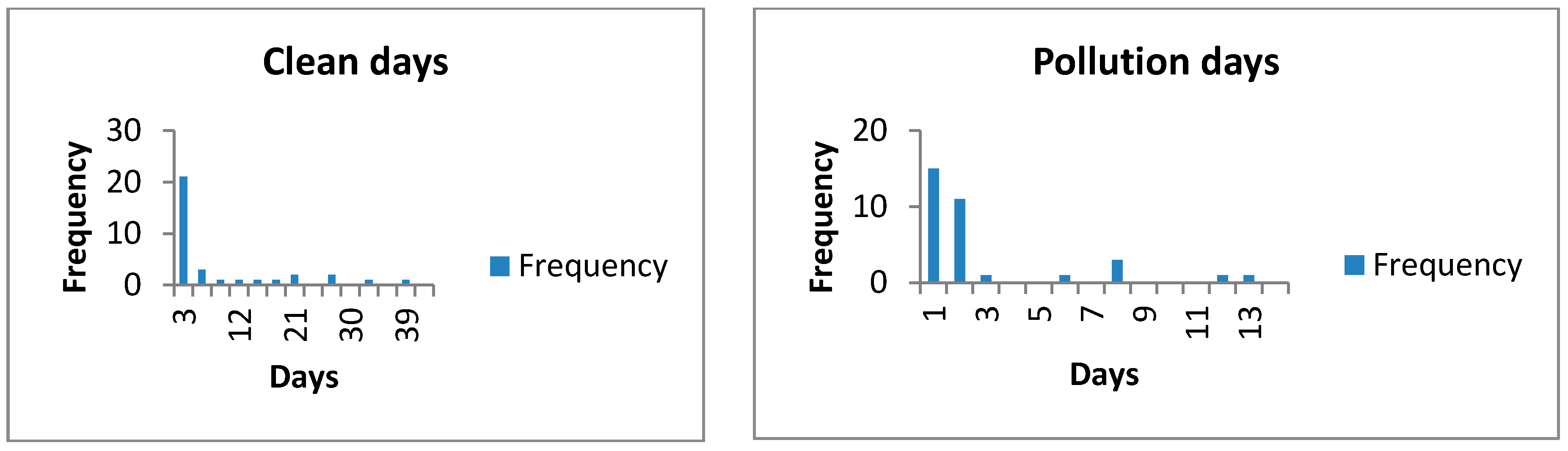
Air conditions affect the EUA spot price under the new scheme. To describe air pollution levels simply, based on a regulation of the UK Department for Environment, Food & Rural Affairs, a clean day is defined as having a daily mean concentration of less than 58 µg/m³, otherwise, it is a pollution day. The frequency of “clean days” and “pollution days” in the UK in 2013 is shown in the following Figure 1.

As Figure 1 shows, “1” denotes clean days and “2” denotes pollution days. The probability distribution of the duration (in days) from clean to pollution (or from pollution to clean) follows an exponential distribution. Thus, we can apply the Markov chain to describe the switching.

4.2. Markovian Switching

The Markovian switching system was first introduced by Krasovskii and Lidskii [20]. This kind of stochastic model describes different types of dynamic systems that might experience abrupt changes in their parameters and structures. The advantages in modelling have been reported in the literature (see Mao [21], Boukas [22], and references therein).

We let $\left(\Omega ,ℱ,{\left\{{ℱ}_t\right\}}_{t\ge 0},\mathbb{P}\right)$ be a complete probability space with filtration ${\left\{{𝓕}_{\mathit{t}}\right\}}_{\mathit{t}\ge \mathbf{0}}$, which satisfies the usual constraints (i.e., it is increasing right-continuous while ${𝓕}_0$ contains all $\mathbb{P}-\mathrm{null}$ sets). Let $r\left(t\right),t\ge 0$ be a right continuous Markov chain on the probability space, which takes values in finite state space $\mathrm{𝕤}=\left\{clean,pollution\right\}$ with the following generator

$$\Gamma =\left(\begin{array}{c}\begin{array}{cc}-v_{cp}& v_{\begin{array}{c}cp\end{array}}\\ v_{pc}& -v_{pc}\end{array}\end{array}\right)$$

Here, $v_{cp}>0$ is the transition rate from the state of “clean” to that of “pollution”, while $v_{pc}>0$ is the transition rate from the state of “pollution” to that of “clean”, and thus,

$$\mathbb{P}\left\{r\left(t+\delta \right)=pollution|r\left(t\right)=clean\right\}=v_{cp}\delta +o\left(\delta \right),$$

and

$$\mathbb{P}\left\{r\left(t+\delta \right)=clean|r\left(t\right)=pollution\right\}=v_{pc}\delta +o\left(\delta \right),$$

where $\delta >0$.

In our case, the Markov chain $r(·)$ is independent of Brownian motion $B(·)$.

As is well known, almost every sample path of Markov chain $r(·)$ is a right-continuous step function [23]. More precisely, there is a sequence ${\left\{{\mathsf{\tau }}_{\mathit{k}}\right\}}_{\mathit{k}\ge \mathbf{0}}$ of finite-valued and ${𝓕}_t$-stopping times, such that $0={\mathsf{\tau }}_0<{\mathsf{\tau }}_1<\dots <{\mathsf{\tau }}_k\to \infty$ almost certainly and $r\left(t\right)$ can be expressed as

$$r\left(t\right)={{\displaystyle \sum }}_{k=0}^{\infty }r\left({\mathsf{\tau }}_k\right)I_{\left[{\mathsf{\tau }}_k,{\mathsf{\tau }}_{k+1}\right]}\left(t\right).$$

Moreover, given that $r\left({\mathsf{\tau }}_k\right)=clean$, random variable ${\mathsf{\tau }}_{k+1}-{\mathsf{\tau }}_k$ follows exponential distribution with parameter $v_{cp}$, namely,

$$\mathbb{P}\left({\tau }_{k+1}-{\tau }_k\ge T|r\left({\tau }_k\right)=clean\right)=e^{-v_{cp}T},\forall T\ge 0,$$

Meanwhile, given that $r\left({\mathsf{\tau }}_k\right)=pollution$, random variable ${\mathsf{\tau }}_{k+1}-{\mathsf{\tau }}_k$ follows exponential distribution with parameter $v_{pc}$, namely,

$$\mathbb{P}\left({\tau }_{k+1}-{\tau }_k\ge T|r\left({\tau }_k\right)=pollution\right)=e^{-v_{pc}T},\forall T\ge 0.$$

We can easily simulate the sample paths of the Markov chain using the exponential distributions.

4.3. Simulation of the Spot Price in the New Trading Scheme

Having reviewed the details of the Markov chain, we now study the SDE MRSRP model with Markov switching. Our aim is to compute the EUA spot prices under the new trading scheme if the firm has to hand many more emissions allowances to the regulator for pollution days. Then, we can compare the spot prices between the current and new trading schemes.

We assume the system parameter $\sigma$ is constant. Given that, on clean days, the parameter $k_c=0.021,$ and on pollution days, the parameter $k_p=0.037$. We estimate the transition rate from clean to pollution using $v_{cp}=0.127$ and the transition rate from pollution to clean using $v_{pc}=0.347$.

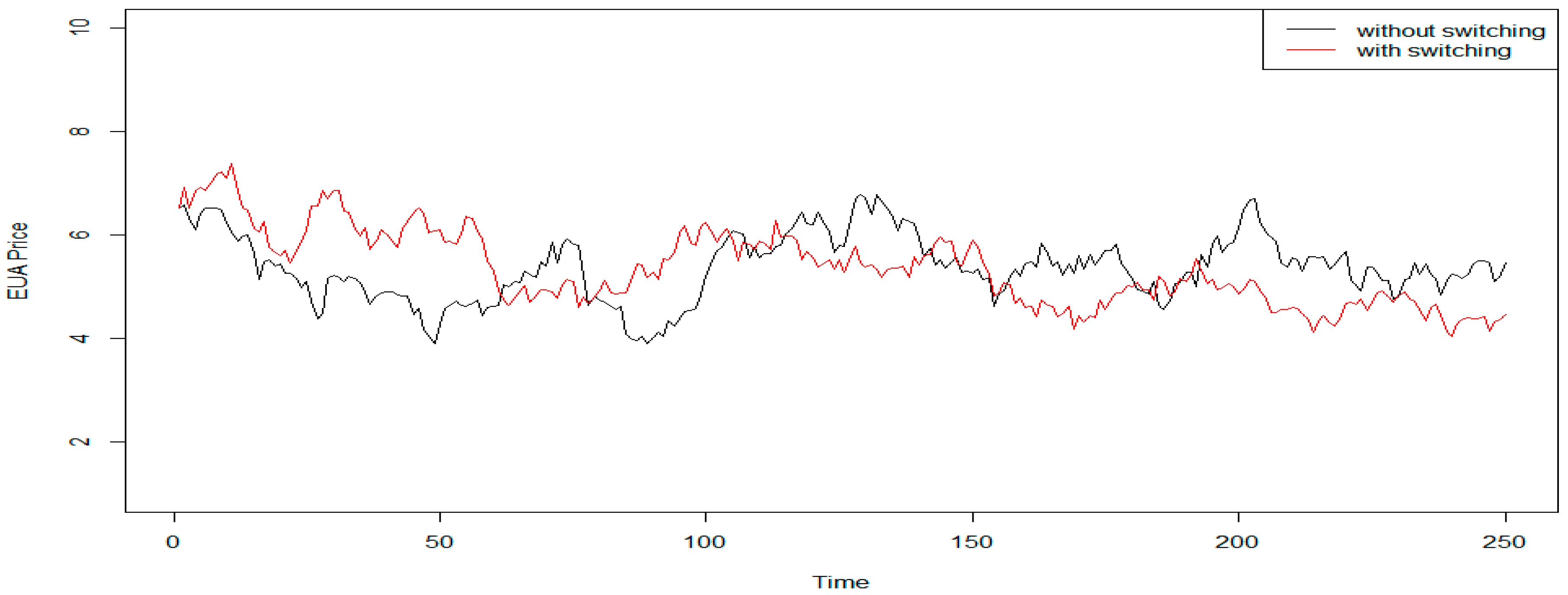
In 2013, there were 250 business days in the EU ETS. Moreover, the starting level of the spot price on 2 January 2013 was 6.52, and we set it as the starting level for 2013, that is, $p_1=6.52$. In this study, we design a function in R-software to perform simulations of the spot price for the SDE MRSRP model (Equation (4)) with Markovian switching with step time $\Delta t=1$. Combined with the spot price of the current scheme without considering the effect of air pollution, we obtain Figure 2.

Figure 2 depicts the computer simulation of the EUA spot price in 2013. The black line is the simulation of the EUA spot price without switching, while the red line is the simulation of the EUA spot price with switching. The former is the EUA spot price under the current EU ETS scheme; the latter is the EUA spot price under the new trading scheme considering the effect of air pollution. As shown in Figure 2, the red line is more stable than the black one. The spot prices do not jump too much under the new ETS. Thus, it would help to improve the ETS and achieve the primary goal—reduction of air pollution by the government at least possible cost.

5. Discussions and Conclusions

This study examines the stochastic nature of emissions allowances under different schemes pertaining to the relevant models that previous studies failed to achieve. First, we analyse the two primary markets for CO₂ emissions allowance spot price under the scheme of the EU ETS: Powernext and ECX. In line with previous studies focused on the EUA spot prices in Phases I and II (e.g., [4,5,6]), the empirical analysis provides evidence that EUA spot prices display non-stationary behaviour in Phase III. In addition, the EUA spot prices approximately follow geometric Brownian motion. An empirical evaluation using actual market data demonstrates that the MRSRP has the best fitness of the five SDEs for representing the dynamics of the EUA spot prices.

More importantly, to reduce smog, this study develops a new scheme in which a firm has to hand many more allowances to the regulator when it emits one unit of air pollution on heavy pollution days, compared to only one allowance on clean days. In Section 4, we show that under the new trading scheme, the air condition can be improved in the pollution days. Using real-life data, we find that the time gap between clean days and pollution days follows exponential distribution, and therefore we develop a SDE MRSRP model with Markovian switching to predict the spot prices in the new trading scheme. The model simulation has shown that the spot prices are expected to not jump too much under the new trading system.

We contribute to the literature in three ways. First, we explore the fitness of the SDEs mainly based on the data of the Phase III of ETS, which has rarely been covered in previous studies. Second, this study is one of the earliest works to develop a new trading scheme with two different states to reduce pollution congestion. The theoretical conception would serve as the basis for more in-depth studies in the future and as a tool for formulating policies aimed at reducing pollution disasters. Third, although a lot of research has been done on spot price modelling, none of the existing literature used SDE with Markovian switching to study the effect of the air condition, and this model is better in our study because there are two different air conditions under our new scheme.

There are several important implications arising from this study for the regulators and managers. First, the current CO₂ emissions market behaves like the MRSRP model. One explanation is that the supply of EUA is fixed in ETS, when there is an increase in demand due to policy or weather conditions, pushing prices higher. When demand returns to normal levels, prices will fall. Besides the mean reverting characteristic, the spot price is proportion to its variance in the current CO₂ emission market [7]. This important property improves the assessment of production costs incorporating CO₂ costs since the introduction of emission trading system, or supports emissions-related investment decisions. The ability of managers to predict the EUA spot prices helps to maintain market efficiency and sustain a healthy trading volume. Second, the estimations in this study showed that the EUA price would not fluctuate too much under the new trading scheme, which greatly enhances the political acceptability of the scheme. Specifically, it implies that the new trading scheme does not lead to more complications in the pricing of emission allowances or to the adverse effect on market liquidity and efficiency. We suggest the government to apply our scheme to upgrade the current trading scheme.

The study has methodological limitations. Primarily, we compare only five SDEs to the EUA spot prices, neglecting other SDEs. In addition, for lack of the EUA price, we cannot compare the theoretical and actual spot price under the new scheme. When future data become available in years to come, it would be worthwhile to re-perform the work in greater detail than the current data allow. Finally, more advanced econometric techniques to estimate the model parameters, including the MCMC method, will be widely elaborated on in the future.

References

1. Paolella, M.S.; Taschini, L. An econometric analysis of emission allowances prices. J. Bank. Financ. 2008, 32, 2022–2032. [Google Scholar] [CrossRef] [Green Version]
2. Daskalakis, G.; Markellos, R.N. Are the European carbon markets efficient? Rev. Futures Mark. 2008, 17, 103–128. [Google Scholar]
3. Oberndorfer, U. EU emission allowances and the stock market: Evidence from the electricity industry. Ecol. Econ. 2009, 68, 1116–1126. [Google Scholar] [CrossRef]
4. Daskalakis, G.; Psychoyios, D.; Markellos, R.N. Modeling CO2 emission allowance prices and derivatives: Evidence from the European trading scheme. J. Bank. Financ. 2009, 33, 1230–1241. [Google Scholar] [CrossRef]
5. Benz, E.; Trück, S. Modeling the price dynamics of CO2 emission allowances. Energy Econ. 2009, 31, 4–15. [Google Scholar] [CrossRef]
6. Seifert, J.; Uhrig-Homburg, M.; Wagner, M. Dynamic behavior of CO2 spot prices. J. Environ. Econ. Manag. 2008, 56, 180–194. [Google Scholar] [CrossRef]
7. Kim, J.; Park, Y.J.; Ryu, D. Stochastic volatility of the futures prices of emission allowances: A Bayesian approach. Phys. A 2017, 465, 714–724. [Google Scholar] [CrossRef]
8. Mills, T.C.; Markellos, R.N. The Econometric Modelling of Financial Time Series, 3rd ed.; Cambridge University Press: Cambridge, UK, 2008. [Google Scholar]
9. Chan, K.C.; Karolyi, G.A.; Longstaff, F.A.; Sanders, A.B. An empirical comparison of alternative models for the short-term interest rate. J. Financ. 1992, 47, 1209–1227. [Google Scholar] [CrossRef]
10. Dotsis, G.; Psychoyios, D.; Skiadopoulos, G. An empirical comparison of continuous-time models of implied volatility indices. J. Bank. Financ. 2007, 31, 3584–3603. [Google Scholar] [CrossRef]
11. Merton, R.C. Option pricing when underlying stock returns are discontinuous. J. Financ. Econ. 1976, 3, 125–144. [Google Scholar] [CrossRef]
12. Dassios, A.; Nagaradjasarma, J. The square root process and Asian options. Quant. Financ. 2006, 6, 337–347. [Google Scholar] [CrossRef] [Green Version]
13. Kourtis, A.; Markellos, R.N.; Psychoyios, D. Wine price risk management: International diversification and derivative instruments. Int. Rev. Financ. Anal. 2012, 22, 30–37. [Google Scholar] [CrossRef]
14. Bierbrauer, M.; Menn, C.; Rachev, S.T.; Trück, S. Spot and derivative pricing in the EEX power market. J. Bank. Financ. 2007, 31, 3462–3485. [Google Scholar] [CrossRef]
15. Detemple, J.; Osakwe, C. The valuation of volatility options. Eur. Financ. Rev. 2000, 4, 21–50. [Google Scholar] [CrossRef]
16. Bahmani-Oskooee, M.; Kutan, A.M.; Zhou, S. Do real exchange rates follow a nonlinear mean reverting process in developing countries? Sou. Econ. J. 2008, 74, 1049–1062. [Google Scholar]
17. Pan, J.; Gray, A.; Greenhalgh, D.; Mao, X. Parameter estimation for the stochastic SIS epidemic model. Stat. Inference Stoch. Process. 2014, 17, 75–98. [Google Scholar] [CrossRef] [Green Version]
18. Rawlings, J.O.; Pantula, S.G.; Dickey, D.A. Applied Regression Analysis: A Research Tool; Springer: New York, NY, USA, 1998. [Google Scholar]
19. European Environment Agency. Air Quality e-Reporting (AQ e-Reporting). Available online: http://www.eea.europa.eu/data-and-maps/data/aqereporting#tab-data-by-country (accessed on 25 January 2017).
20. Krasovskii, N.N.; Lidskii, E.A. Analysis design of controller in systems with random attributes—Part 1, Automat. Rem. Control 1961, 22, 1021–1025. [Google Scholar]
21. Mao, X. Exponential stability of stochastic delay interval systems with Markovian switching. IEEE Trans. Autom. Control 2002, 47, 1604–1612. [Google Scholar]
22. Boukas, E.K. Stabilization of stochastic nonlinear hybrid systems. Int. J. Innov. Comput. Inf. Control 2005, 1, 131–141. [Google Scholar] [CrossRef]
23. Anderson, W.J. Continuous-Time Markov Chains; Springer: Berlin/Heidelberg, Germany, 1991. [Google Scholar]
Figure 1. UK air condition in 2013 [19].
Sustainability 09 00207 g001
Figure 2. Comparison of EUA spot prices under different schemes.
Sustainability 09 00207 g002