The Monetary Valuation of Environmental Externalities through the Analysis of Real Estate Prices

Abstract

This paper proposes a theoretical model of evaluation of environmental externalities based on the analysis of real estate prices. This issue is included in regional planning policies which include activities and interventions that produce economic and non-economic effects. The monetary assessment of economic and non-economic effects can be expressed as a forecast (ex ante) and/or following (ex post) such activities and interventions. The assessment of the economic impact, with particular reference to interventions and infrastructure work, is widely based on procedures which make use of market prices. The proposed model was applied to an actual case, considering the effects of noise pollution, produced by traffic from the Naples Beltway, on residential property.

1. Introduction

Among the monetary valuation methods of environmental externalities is the econometric analysis of real estate prices (Land Price Analysis), the logical basis of which lies in the principle that the price of real estate is affected, among other things, by the quality of the environment [1,2,3,4,5,6,7,8,9,10,11,12]. This principle postulates that properties are “receptors” of environmental externalities, which, in the same way as positional rents, are incorporated into the market prices [13]. This makes it possible to estimate the value of environmental externalities equal to the measure of the change in housing prices resulting from environmental change. The estimation can be carried out using statistical pluriparametric models (e.g., multiple regression or semiparametric models), which are able to define the market price as a function of the variables corresponding to the property’s characteristics, including those relating to the environmental qualification of the territory [14,15,16,17,18,19,20,21,22,23,24].

This study aims to evaluate the environmental externalities through the analysis of real estate prices. In particular, it is proposed to define the evaluation scheme that allows

• determining the non-marginal changes in real estate related to the quality characteristics of the environment. This change corresponds to the “rank” to be attributed to these characteristics in order to calculate the price differences of property that are produced by environmental changes caused by the transformation of the territory;
• taking into account the contribution to the change in price of factors other than environmental variables, for example by changing the intrinsic property characteristics originated from the transformation of the environment.

The analysis of real estate prices to evaluate environmental externalities is described in stages in the first part of this study. In formal logic terms, the function of estimating externalities in relation to the main algebraic forms used in the econometric analysis of the housing market is laid out below. In formal logic terms, for ex ante and ex post evaluations, the calculation of the variation of the real estate properties is also intended for the assessment of the effects on property prices generated by environmental changes.

2. Methods

2.1. Steps of the Analysis

The analysis of real estate prices leads to the evaluation of environmental externalities through an articulated operational scheme.

Once the area under study, intended as the area affected by environmental changes, has been defined, different homogeneous categories of properties should be identified (houses, agricultural land, building soils, industrial and commercial buildings, etc.). For each category (j = 1, 2, …, n), an adequately representative sample is defined (c_j); the phases are:

(1)

Determination of the price change (ΔPK_ji = 1, 2, …, c’_j) that produces environmental modification on the properties of the sample;

(2)

Aggregation of the price change (ΔP_j) in every single property category;

(3)

Determination of the monetary value of environmental externalities (W_e).

The implementation of the first phase involves the search of G_j function such that:

ΔPK_ji = G_j(Δx_v)

(1)

In this function, Δx_v represents the variation in the quantity (or the degree of manifestation) of the variables (x_v, v = 1, 2, … r) that express the (extrinsic) characteristics of the property regarding the environmental qualification within the territory under study (presence of spaces designed for public parks and gardens, people-friendliness, aesthetic and visual conditions of the landscape, etc.). The Δx_v variance, evidently, is derived from comparing the state of the area before an environmental change with the state of the area in the situation after the environmental change. The variables are given by the environmental characteristics that are influenced, positively and/or negatively, by the interventions on the territory. The calculation of the AP_j price change (second phase), in turn, may be based on the average value (μ_j) of changes in the price of real estate, p_j [25]. This value must be determined by an estimate, by range, conducted on the arithmetic mean (m_j = ∑_j ΔPK_ji /c’_j) of changes in the price of the real estate c_j sample. This may be achieved through the following relation:

µ_j = m_j ± Zs/(c’_j)^1/2,

(2)

where Z represents the stochastic variable resulting from the variable V_j (v_j = ΔPK_ji) through the following report: z = (v_j − µ_j)/s; s is the standard deviation of changes in the price of the real estate sample, c_j. In this way, the calculation of ΔP_j may conservatively be made on the basis of the minimum value µ_j resulting from the estimate by range:

ΔP_j = µ_{j min ·} p_j.

(3)

Lastly, in the final phase, the monetary value of environmental externalities can be determined as the sum of ΔP_j changes extended to the various populations of properties located in the study area:

W_e = ∑_j ΔP_j.

(4)

2.2. The Function of Estimate

The practical applicability of the outlined operational framework is obviously subject to the ability to determine the changes in real estate prices, produced by environmental change. Formally, the calculation could be done using the G_j function that relates the price of real estate with the environmental variables (F_j). The application of econometric models in search of the F_j function is however conditioned by the data collection mode, implying the construction of an estimate-statistical sample, the determination of market prices and the environmental characteristics of the buildings, both in the situation with and in the situation without intervention.

2.3. Data

The collection of data may present fewer difficulties when the evaluation of externalities is performed ex post, i.e., after the execution of activities and interventions. In particular, when the effects of activities and interventions only partially affect the area under study, i.e., by the presence of zones that represent the situation with interventions and of zones that retain the conditions of the situation without interventions, it becomes possible to determine the market price of the real estate in both situations, and thus the value of the environmental characteristics. The lack of references to the situation prior to the execution of activities and interventions—e.g., in cases of global redevelopment of old towns, the total reclamation of degraded sites, etc.—implies, of course, operational problems of greater complexity. Here, the correct solution can be found when the data relating to the situation without intervention is deduced through the price analysis of properties located in areas with environmental characteristics similar to those that originally qualified the transformed territory. In ex ante evaluations, the construction of the estimate-statistical sample is instead usually conditioned by the absence of basic data on the situation with intervention. It follows that the determination of the elements necessary for the construction of the sample involves the examination of the prices and characteristics of properties located in areas that display the specific environmental qualities that the area under study may assume, as a result of the interventions. It goes without saying that the areas compared, as far as is possible, must be subject to similar actions and interventions. When this condition cannot be met, the construction of the estimate-statistical sample must be adequate in order to support the definition of an econometric function able to represent the trend in the price of real estate located on the territory under study. This is estimated in relation to different degrees of manifestation of environmental characteristics (amount of pollutants in the atmosphere, intensity of disturbing noise from vehicular traffic, availability of recreational areas, etc.). The data, therefore, must be collected from geographical areas with varying environmental qualities that differ from the area under study, but that are similar to the area under study with regard to the market character and nature and consistency of the property. Both in ex ante and ex post evaluations, comparable data should be collected in order to eliminate variations that can be ascribed to factors other than environmental externalities. The aim is, of course, to arrive at differential rates of value attributable coeteris paribus to the variations of environmental quality. In any case, the construction of the sample should take into account possible differences in the regulation of property transaction conditions. This can be achieved by appropriately adjusting the price of comparable real estate, according to the operators’ economic trend in the market under study. The statistical analysis of the sample allows to obtain the parameters of econometric price function as estimated values of the regression coefficients.

2.4. The Algebraic Relationship

The price function, defined for each property category located in the area under study, can be expressed symbolically as follows:

PK_ji = (x_v, x_jt)

(5)

PK_ji expresses the market price of generic property, x_v (v = 1, 2, …, r) represent the environmental variables, and x_jt, (t = 1, 2, …, s) indicate the remaining variables that contribute to the formation of real estate prices, and that, in general, relate to

• the extrinsic property characteristics related to location (accessibility to tertiary activity area, distance from the main traffic lines, etc.);
• the intrinsic characteristics of the property related to the position (front, orientation, panoramic views, etc.).
• the technological characteristics (systems, qualities, etc.);
• the production characteristics (whether the property is rented, exempted from tax payment, its level of productivity of agricultural land or building capacity, etc.).

The time of sale of real estate can also be understood to be a x_jt variable. This variable is normally used as a temporal reference to take into account price changes due to the inflationary process or other market contingencies. Using the F_j function, the price change of the property is calculated in discrete terms, i.e., it must be determined as the difference of function values obtained by assigning the measure to the environmental variables, both in the situation with (x_vp) and in the situation without (x_va) intervention. The quantification of the variables must be operated on the basis of the measurement system (techniques, dichotomous measures, scores, etc.). If this function is linear and environmental variables are represented by rating scales, the price change can be calculated as the sum of the implicit marginal prices of the same variables, namely the algebraic sum of the price changes due to differences of variables taken individually. In the remaining cases, the price change must be determined by simultaneously introducing—in function—the environmental variables in accordance with the respective values x_vp and x_va. It is clear that the mathematical formulation of the price change, and consequently the symbolic expression of the G_j function, depends on the algebraic structure of the function price F_j. Assuming, as an example, that F_j has one of the three forms of function—linear, multiplicative or exponential—which represent the most commonly used functional dependencies in the econometric analysis of the housing market, it follows that the price change is given by the following equations:

F_j linear (PK_ji = ∑_t a_jt x_jt + ∑_v a_v x_v): ΔPK_ji = ∑_v a_v (x_vp − x_va)

(6)

F_j multiplicative (PK_ji = ∏_t x^ajt_jt + ∏_v x^av_v): ΔPK_ji = ∏_t x^ajt_jt ∏_v (x^av_vp − x^av_va)

(7)

F_j exponential (PK_ji = e^∑_t^{ajtxjt + ∑tavxv}): ΔPK_ji = e^∑_t^ajtxjt (e^∑_v^vavxvp − e^∑_v^vavxva)

(8)

In these equations, a_v and a_jt are respectively the regression coefficients of the environmental variables (x_v) and the remaining endogenous variables (x_jt) of the price function. The calculation of the price change also requires the determination of the amounts of the x_v environmental variables in the previously existing situation and in the one subsequent to the implementation of interventions. This problem must be resolved in different ways, depending on whether the evaluation of externalities is carried out in ex ante or ex post conditions.

2.5. Ex Ante Evaluation

The assessment of externalities in the ex ante condition (forecast) involves a determination of price changes that will occur on real estate as a result of the environmental changes generated by according interventions [26,27,28,29]. This operation, as already mentioned, may be affected via the G_j estimation function, which requires the calculation of the x_v environmental variables in situations with and without intervention. In ex ante evaluations, only the amounts of environmental variables related to the phase previous to the interventions (x_va) are known a priori; future amounts are unknown: namely, the values that the variables assume as a result of environmental changes caused by according activities and interventions (x_vp). The forecast of future values of environmental variables is certainly a complex problem that does not have a univocal solution. It can have a probabilistic solution. In this case, the determination of the values that tend to occur under risk must be distinguished from the estimated values under conditions of uncertainty. Risk conditions, as is known, arise in the presence of probabilistic elements relevant to the investigated variables. The uncertainty when forecasting the unknown values comes about in the absence of data on which to base the calculation of probability of their occurrence.

The ex ante assessment of environmental externalities is mainly used in the economic analysis of intervention projects on the land, and in particular in the sectors of water resources [27], atmospheric depollution [25,26] and noise depollution [28,29]. More recent studies have considered the contingent valuation method to determine the depreciation of agricultural soils following the possible construction of overhead electrical power lines (in terms of risk perception by electromagnetic fields) [30], or genetic algorithms to determine the territorial impact (in terms of market depreciation for buildings and lands) caused by high-speed railway varying its possible paths [31].

2.6. Assessment in Risk Condition

Under risk, the future amounts (x_vp) of the generic environmental feature x_v, in probabilistic terms, can be determined as an expected value or a mathematical expectation of the stochastic variable (X_vp) with amounts corresponding to the possible “states” that the characteristic x_v may take on as a result of interventions (a more or less high level of healthy air, the usability of natural resources, aesthetic and visual quality of the landscape, etc.). The measures of each environmental characteristic under analysis, which might occur as a result of the interventions (S_vn, n = 1, 2, 3, … , u) and the respective probability of occurrence (p_n) must be defined for comparison with initiatives which have already been implemented, similar to the one that is to be carried out on the area under study. In practice, the S_vn measures must be identified by examining the nature and magnitude of the effects that the comparison initiatives have produced in areas which originally had environmental characteristics similar to those of the area under study. p_n chances, in turn, can be obtained “objectively” by the frequencies (f_n) assigned to the S_vn measures, based on the experiences examined, the result being:

∑_n p_n = 1

(9)

This equivalence excludes the presence of any residual uncertainty or unforeseen circumstance in the estimation of the future value of the environmental feature taken into consideration. Once the S_vn measures and p_n probabilities are known, it is possible to calculate the expected value of the X_vp variable_. It is therefore given that (x_vp1, x_vp2, …, x_vpu) are the values of the X_vp variable in ascending order, and that p_n (n = 1, 2, 3, …, u) corresponds to relative probabilities, which are determined by assuming, for practical purposes:

p_n (X_vp = x_vpn) = f_n (x_vpn)

(10)

the expected value M(X_vp) of the X_vp variable will be equal to:

M(X_vp) = ∑_n [x_vpn ∙ f_n (x_vpn)]

(11)

It is a value which represents, by definition, a forecast of the X_vp variable and that expresses the future amount attributed to the x_v characteristic for calculating the change in the price of real estate. It is also clear that the extent of this change depends on the M(X_vp) value by means of the econometric function G_j. Thus, the “expected value” of the change can be determined using the following relation:

E[G_j(X_vp)] = ∑_n [G_j(x_vpn) ∙ f_n (x_vpn)],

(12)

where E is the mathematical expectation, and E[G_j(X_vp)]—because it is the application of this parameter to the G_j(X_vp) function—expresses the expected value.

The calculation of the expected value becomes simple if the G_j(X_vp) function is linear:

G_j(X_vp) = ΔPK_ji = ∑_n a_v x_vp − b

(13)

and because b = ∑_v a_v x_va is known, for the mathematical operator linearity that defines the mathematical expectation, it can be set out as:

E[G_j(X_vp)] = ∑_v a_v x_va E(X_vp) − b.

(14)

This report provides, in a simplified way, the expected property prices.

2.7. Assessment in Condition of Uncertainty

The evaluation of externalities under risk uses probabilistic evidence regarding the future conditions of environment characteristics. Sometimes, however, the analytical elements, such as the future connotations of the intervention area, cannot be obtained due to a lack of appropriate references. The uncertainty of the prediction of the “expected value” of the environmental characteristics increases and is reflected on the determination of the price change of the property. The solution to the problem is the hypothesis of equiprobability of future states of the analysed characteristics. It relies on the principle of insufficient reason that, used with the support of the probability calculus, is attributed to Bayes. In relation to the subject matter, the principle of insufficient reason can be thus expressed: in the absence of information on the probability of future states of the environmental characteristics, and since there is no reason to believe that one of the conditions is more likely than another, it is legitimate to assume that all conditions have the same probability of occurrence, therefore they are equally probable. In the estimation of the “expected value” of the environmental characteristics of the area of intervention, the hypothesis of equiprobability implies that only the future conditions of each feature are taken into account. These are to be identified in relation to the type and size of the works to be carried out, the initial quality of the area and to the impact that interventions will likely generate on the environment. Based on the assumption of equiprobability, having indicated the amounts of the random variable, X_vp that correspond to the equally likely states (p) of the environmental characteristic x_v, with x_vpn (n = 1, 2, …, u) one comes to:

M(X_vp) = ∑_n [x_vpn ∙ p(x_vpn)].

(15)

For the calculation of the real estate price change, the “expected value” of the X_vp variable must be attributed to the x_v environmental feature.

2.8. The Role of the Intrinsic Property Features

Until now, the hypothesis was made whereby the change in property prices is related solely to the change in environmental characteristics, which can be considered extrinsic factors that influence the value of the properties. The changes to the environment resulting from the interventions in the territory, however, can also affect the intrinsic character of the buildings and cause positive or negative effects on their market prices. The evaluation of environmental externalities must also take these effects into account. It must consider the consequences of all the variations that environmental change will bring on the real estate prices. The problem arises when, among the endogenous variables of the price function, there are also intrinsic factors subject to variation due to environmental externalities. The problem does not arise when the price is statistically independent from the intrinsic factors. Intrinsic factors of real estate, which the transformation of the environment can influence, are mainly positional (panoramic views, brightness, etc.) and technological-productive (maintenance, fertility of agricultural soils, etc.). There is no doubt that a positive environmental change, due to an improvement in the healthiness of the air, for example, can have a positive impact on the panoramic views and the brightness of the property, as it can also slow the process of deterioration of some elements of buildings (plastering, etc.). Similarly, deterioration in the quality of the air can have a negative impact on the same property characteristics. In the case of modifications of the intrinsic character of the property due to the transformation of the environment, the price change ΔPK_ji should be calculated as per usual through the econometric function G_j, which can be represented with the following reports:

F_j linear (PK_ji = ∑^s’_{t = 1} a_jt x_jt + ∑^s_{t = s’ + 1} a_jt x_{jt +} ∑_v a_v x_v):
ΔPK_ji = ∑^s’_{t = 1} a_jt (x_jtp − x_jta) + ∑_v a_v (x_vp − x_va)

(16)

F_j multiplicative (PK_ji = ∏^s’_{t = 1} x^ajt_jt + ∏^s_{t = s’+1} x^ajt_jt + ∏_v x^av_v):
ΔPK_ji = ∏^s’_{t = 1} (x^ajt_jtp − x^ajt_jta) ∏^s_{t = s’ + 1} x^ajt_jt ∏_v (x^av_vp − x^av_va)

(17)

$$F_{j}exponential\left[P{K}_{ji}=e^{\left({\displaystyle \sum _{t=1}^{s^{\prime }}{a}_{jt}{x}_{jt}+}{\displaystyle \sum _{t=s^{\prime }+1}^s{a}_{jt}{x}_{jt}+}{\displaystyle \sum _v{a}_v{x}_v}\right)}\right]$$

(18a)

$$\Delta P{K}_{ji}=e^{{\displaystyle \sum _{t=s^{\prime }+1}^s{a}_{jt}{x}_{jt}}}\left[e^{\left({\displaystyle \sum _{t=1}^{s^{\prime }}{a}_{jtp}{x}_{jtp}+{\displaystyle \sum _v{a}_v{x}_{vp}}}\right)}+e^{\left({\displaystyle \sum _{t=1}^{s^{\prime }}{a}_{jta}{x}_{jta}+{\displaystyle \sum _v{a}_v{x}_{va}}}\right)}\right]$$

(18b)

The x_jt variables, with t = 1, 2, …, s’ (s’ < s), represent the intrinsic property characteristics affected by environmental changes. x_jtp and x_jta indicate values to be assigned to the variables in situations with and without intervention; this comparison allows for the calculation of the change in property prices. In ex ante evaluations, x_jta values are obviously known a priori. By contrast, the x_jtp values are unknown; they should be determined taking into account the weight that is exercised exclusively by environmental externalities on variables x_jt (t = 1, 2, …, s’) and not by other factors (technological, commercial, etc.). For the assessment, the basic assumptions are:

x_jtp = (x*_jtp − x’_jtp),

(19)

where x*_jtp represents the amount of x_jt character, in the situation with, and x’_jtp without environmental externalities. The expected value of x_jtp is then given by:

E(X*_jP − X’_jP) = E(X’_jP) − E(X’_jP)

(20)

where E is the mathematical expectation operator and X*_jtP and X’_jtP are random variables that describe the possible x*_jtp and x’_jtp values, attributable to the characteristics of real estate x*_jt (t = 1, 2, …, s’). By calculating E(X*_jP) and E(X’_jP), X_jtP can then be predicted, depending on the availability of probabilistic elements concerning the variables X*_jtP and X’_jtP, under risk or in conditions of uncertainty.

2.9. Ex Post Evaluation

The ex post evaluation of environmental externalities requires that the price of a property changes due to environmental changes. It is clear that this variation should not be determined by a simple comparison of real estate prices in the two situations before and after interventions. This is because the price of real estate in the situation after intervention can be an expression not only of environmental change but also of other causes, such as the dynamics of demand and supply of real estate or any technological and structural upgrading activities on the buildings, etc. For the evaluation of externalities, it is therefore necessary to isolate the contribution that environmental changes alone have on changes in property prices. The econometric G_j function should be developed by adapting the amounts of the environmental variables in relation to the conditions with and without intervention (x_vp and x_va). The function should also be adapted based on the amounts of the intrinsic characteristics of the properties x_jt (t = 1, 2, …, s’)—production and position—which undergo the effect produced by transformation of the environment.

3. Literature Review about Noise Pollution Effects on Residential Real Estate Values

Noise pollution due to road traffic is often added to other existing generalized pollution sources. This causes a deterioration of urban quality, often already partially compromised in environmental terms. For noise pollution, the real estate values are subject to low marketability, because real estate goods are complex assets linked to many factors, including infrastructural, urban and environmental quality. The economic effects derived from road traffic have led to investment in extremely complex aspects, yet still they represent a research issue. Several studies have been conducted in order to determine the monetary value of environmental externalities in transport and vehicular traffic sectors.

A literature review relating to these issues was reported in a study of Navrud [32], where main studies from the 1970s until 2001 are cited. Most recent studies, until 2011, are cited in Del Giudice and De Paola [33,34]. The results of these studies and of a more recent one [35] are summarized in

Table 1. Literature review.

Authors	Year	Study Location	Average Reduction of Real Estate Values for an Unit Increase of Noise Pollution (dB)
Gamble et al.	1974	Bogota, Rosendale, North Springfield; USA	0.73%
Hammar	1974	Stockholm; Sweden	1.25%
Vaughan and Huckins	1975	Chicago; USA	0.65%
Langley	1976	North Springfield, VA; USA	0.22%
Anderson and Wise	1977	Towson; North Springfield; USA	0.29%
Bailey	1977	North Springfield; USA	0.30%
Hall et al.	1978	Toronto; Canada	1.05%
Nelson	1978	Washington D.C.; USA	0.87%
Allen	1980	North Virginia, Tidewater; USA	0.15%
Palmquist	1980, 1981	Kingsgate, North King, Spokane; USA	0.29%
Hall et al.	1982	Toronto (Arterial Expressway); Canada	0.47%
Pommerherne	1986	Basel; Switzerland	1.26%
Iten and Maggi	1990	Zurich; Switzerland	0.90%
Soguel	1990	Neuchatel; Switzerland	0.91%
Hidano et al.	1992	Tokyo; Japan	0.70%
Vainio	1995	Helsinki; Finland	0.36%
Renew	1996	Brisbane; Australia	1.00%
Grue et al.	1997	Oslo; Norway	0.33%
Wilhelmsson	2000	Stockholm; Sweden	0.60%
Lim and Ko	2001	Bucheon; Korea	0.30%
Bateman et al.	2001	Glasgow; UK	0.20%
Huang and Palmquist	2001	Seattle; USA	0.56%
Stanley and Autroads	2001	Australia	0.50%
Nelson	2004	Toronto; Canada	0.55%
Theebe	2004	Amsterdam, Alkmaar, Utrecht, Rotterdam; Holland	0.40%
Rich and Nielsen	2004	Copenhagen; Denmark	0.51%
Baranzini and Ramirez	2005	Geneva; Switzerland	0.64%
Janmaat	2005	Nova Scotia; Canada	1.20%
Day et al.	2006	Glasgow; UK	0.31%
Kim, Park and Kweon	2007	Seoul; Korea	1.30%
Nelson	2007	[Comparative bibliographic analysis]	0.50%
Day et al.	2007	Birmingham; UK	0.35%
Dekkers and Van der Straaten	2008	Amsterdam; Holland	0.16%
Andersson, Jonsson and Ogren	2010	Lerum; Sweden	1.45%
Blanco and Flindell	2011	London, Birmingham, Sutton Coldfield; UK	0.45%
Brandt and Maennig	2011	Hamburg; Germany	0.23%
Chang and Kim	2013	Seoul; Korea	0.53%

.

Sample size, algebraic function, explanatory variables and reference sound level, are aspects that differentiate the case studies of literature.

Regarding case studies, two main approaches can be recognized in literature. The first approach concerns the estimation of average annual percentage variation for residential real estate values for every decibel produced by road traffic by hedonic price models [36,37,38,39,40,41,42]. The second approach is based on willingness to pay for the reduction of the noise level produced by road traffic, also considering an annual economic value per person disturbed by noise [43,44,45,46].

Here, in accordance in the first approach, a hedonic price model, based on a generalized additive model, has been implemented for the estimation of property price reduction caused by noise pollution of the Naples Beltway.

In particular, the existing relationship between property price (y_j) and real estate characteristics x_i (i = 1, …, n) has been expressed by a generalized additive model as follows [47,48,49,50]:

$$P=y_j={\mathsf{\beta }}_0+{\mathsf{\beta }}_1{x}_1+.....+{\mathsf{\beta }}_k{x}_k+f_{k+1}\left(x_{k+1}\right)+.....+f_n\left(x_n\right)+\mathsf{\epsilon }$$

(21)

where β_i and ε are, respectively, the marginal prices and error term.

For the model’s non-linear components, the penalized spline functions have been used:

$$f(x)={\mathsf{\alpha }}_0+{\mathsf{\alpha }}_{1}x+.....+{\mathsf{\alpha }}_p{x}^p+{\displaystyle \sum _{z=1}^Z{\mathsf{\alpha }}_{pz}{{(x-k_z)}^p}_{+}}$$

(22)

where the generic function (x − k_z)^p₊ has (p − 1) continuous derivatives.

4. Case Study

4.1. Noise Pollution Surveys

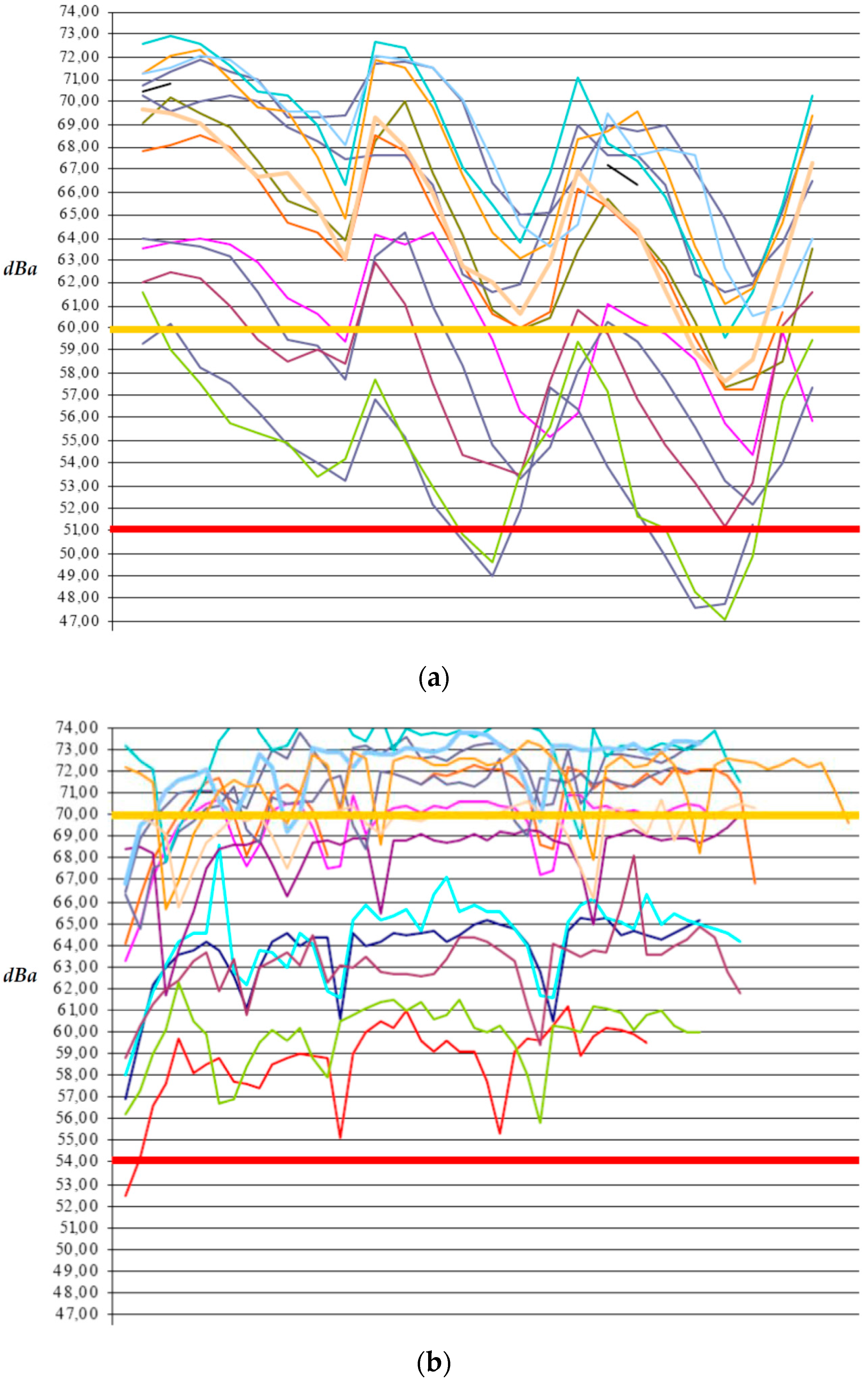
The monitoring of noise pollution has identified the sound pressure equivalent levels (Leq) by two consequential phases: In the first phase of the survey, the background noise (diurnal and nocturnal) was identified. It is also definable as the noise generated by n − 1 factors present in the urban area of interest with the exception of noise emissions generated by the Naples Beltway. In the second phase, the sound pressure levels were detected, in continuous mode (24 h a day), in correspondence with 14 residential units located at a minimum of 7 m up to a maximum of 49 m from the Beltway’s axis.

In accordance with a comparative criterion provided by Italian law, measurement results of the second phase have been compared with background noise levels (diurnal and nocturnal) determined in the first phase, observing eventual excessive noise emissions produced by the Naples Beltway over background noise levels (diurnal background noise equal to 50.7 dB, nocturnal background noise equal to 47.5 dB). Italian law stipulates that the normal tolerability of noise emissions is exceeded when noise is 3 dB over background noise.

Analysing the survey’s results, the sound pressure levels for each measurement point were consistently higher than the diurnal and nocturnal tolerability limits as determined by the comparative criterion above (see Figure 1). Noise measurements and noise tolerability limits are graphically represented in Figure 1, where the yellow line is the average noise level and the red line is the background noise level.

4.2. Model’s Specification

The model’s algebraic structure has been specified on the basis of estimation tests of empirical-argumentative nature:

$$PRICE={\mathsf{\beta }}_0+{\mathsf{\beta }}_{1}floor+{\mathsf{\beta }}_{2}lift+{\mathsf{\beta }}_{3}main+{\mathsf{\beta }}_{4}bath+{\mathsf{\beta }}_{5}qu+f_1(retarea)+{\mathsf{\epsilon }}_i$$

(23)

The dependent variable (PRICE) coincides with property prices. The other independent variables are the following:

• floor level (floor), with values from 0–9;
• presence of lift (lift), expressed by a dichotomous scale (1 if present, 0 if absent);
• status of maintenance of the real estate properties (main), assigning 1 or 0, respectively, if housing units are recently renovated or to be renovated;
• number of bathrooms (bath), with values from 1–3;
• urban quality (qu), expressed by a proxy variable (assigning 1 if the Naples Beltway is adjacent to housing units or if housing units are within a radius of 100 meters to the Beltway limit, 0 otherwise);
• retail area of the housing unit (retarea) expressed in square meters.

All the sampled housing units (46 real estate transactions) have similar quality and are located in the same neighbourhood where the housing units are already subject to noise monitoring (central area of Naples).

4.3. Model’s Results

Without the effects of multicollinearity, the main indices of the model are shown in

Table 2. Statistic sample description and main results of the model with respect to floor level (floor; 1–9); the presence of a lift (lift; 1/0); status of maintenance (main; 1/0); number of bathrooms (bath; 1–3); urban quality (qu; 1/0); retail area of the housing unit (retarea; m²).

Characteristics	Average	Median	Min	Max	Std. Dev.
Price	€483,392	€494,760	€217,000	€911,400	€171,601
retarea	117.39 m2	110.00 m2	60.00 m2	220.00 m2	43.61 m2
floor	2.52	2.00	0.00	9.00	2.77
lift	—	1.00	0.00	1.00	—
main	—	1.00	0.00	2.00	—
bath	—	2.00	1.00	3.00	—
qu	—	0.00	0.00	1,00	—
Linear Components	Coef	Std. Error	Ratio	p-Value
constant	57.300	66.700	0.8591	0.3916
floor	16.800	2.664	6.3080	0.0000
lift	57.650	20.780	2.7740	0.0062
main	17.640	9.480	1.8610	0.0646
bath	22.760	21.200	1.0740	0.2846
qu	−20.100	16.340	−1.2300	0.2204
Non-Linear Component	df	Spar		Knots
retarea	2	2.691		5.0000

. The estimated values show a trend in line with the observed data; furthermore, the residual analysis shows no anomalies. The determination index is equal to 0.988 and the F-test is statistically significant with a 95% confidence level. The only non-linear component of the model is statistically significant because there are no anomalies for the degrees of freedom (df) and smoothing parameter (spar). On the other hand, some linear components are significant for a confidence level below 95% (p-value), but they have not been excluded from the analysis for non-statistic reasons based on their importance in the constitution of property prices. The marginal price for urban quality (qu) has a negative sign and is equal to €20,100, showing that noise pollution due to road traffic leads to a significant reduction of property prices (about 4.16% on the average price of the real estate sample). The trend of other components of the model is only shown graphically (Figure 2), the primary objective of this analysis being the elicitation of the urban quality variable as an environmental externality.

The reduction of residential real estate values can be determined assuming that the amount of the urban quality variable (marginal price) corresponds to the average sound levels (diurnal and nocturnal) detected by noise monitoring.

The diurnal and nocturnal noise limits for different units examined are known, (in particular, the diurnal noise range from 58.8 dB to 73.1 dB and the nocturnal noise range from 53.8 dB to 68.5 dB), for which we can define the open interval of noise related to the marginal price of the urban quality variable (58.8 dB–73.1 dB for diurnal noise; 53.8 dB–68.5 dB for nocturnal noise).

The average noise levels of the above intervals have been considered in order to obtain a prudential value in the event of real estate sale for each housing unit subject to phonometric measurements.

The reduction of residential real estate values (D) can be determined as follows:

D = max (D_DIURN, D_NOCT)

(25)

with:

D_DIURN = [p_qu/(LeqMD−LeqTD)] x (LeqD−LeqTD)

(26)

D_NOCT = [p_qu/(LeqMN−LeqTN)] x (LeqN−LeqTN)

(27)

where p_qu is the marginal price of the urban quality proxy variable; LeqMD and LeqMN are the average equivalent sound pressure levels, diurnal and nocturnal for the sampled real estate units, respectively; LeqTD and LeqTN are the noise tolerability limits, diurnal and nocturnal, respectively; LeqD and LeqN are the average noise levels (diurnal and nocturnal) for each housing unit subject to phonometric measurements.

The main results of phonometric surveys and the reduction of real estate values for housing units subject to noise monitoring are shown in

Table 3. Main results of phonometric surveys.

Sample	Equivalent Sound Level—Leq (dB)		Depreciation for 67.7 dB (Diurnal Emissions) and 63.2 dB (Nocturnal Emissions)
	Average Diurnal Value (LeqD)	Average Nocturnal Value (LeqN)
Subject 1	70.3	67.2	€20,100.00
Subject 2	69.3	64.3	€20,100.00
Subject 3	63.2	58.4	€20,100.00
Subject 4	64.4	58.8	€20,100.00
Subject 5	70.7	66.3	€20,100.00
Subject 6	59.9	54.5	€20,100.00
Subject 7	69.6	64.7	€20,100.00
Subject 8	73.1	68.2	€20,100.00
Subject 9	68.3	63.8	€20,100.00
Subject 10	58.8	53.8	€20,100.00
Subject 11	72.2	67.6	€20,100.00
Subject 12	71.5	67.9	€20,100.00
Subject 13	63.9	60.2	€20,100.00
Subject 14	72.0	68.5	€20,100.00

,

Table 4. Reference average intervals of phonometric surveys.

	Day	Night
Min	58.8	53.8
Average	67.7 (LeqMD)	63.2 (LeqMN)
Max	73.1	68.5

and

Table 5. Reduction of real estate values for housing units.

Sample	Depreciation-Diurnal Emissions		Average Diurnal Depreciation		Depreciation-Nocturnal Emissions		Average Nocturnal Depreciation
Subject 1		€23,832.86		5.47%		€26,430.71		5.47%
Subject 2		€22,397.14		4.52%		€21,840.94		4.52%
Subject 3		€13,639.29		2.59%		€12,503.15		2.59%
Subject 4		€15,362.14		2.72%		€13,136.22		2.72%
Subject 5		€24,407.14		5.17%		€25,006.30		517%
Subject 6		€8901.43		1.31%		€6330.71		1.31%
Subject 7		€22,827.86		4.65%		€22,474.02		4.65%
Subject 8		€27,852.86		5.80%		€28,013.39		5.80%
Subject 9		€20,961.43		4.35%		€21,049.61		4.35%
Subject 10		€7322.14		1.08%		€5222.83		1.08%
Subject 11		€26,560.71		5.60%		€27,063.78		5.60%
Subject 12		€25,555.71		5.70%		€27,538.58		5.70%
Subject 13		€14,644.29		3.18%		€15,351.97		3.18%
Subject 14		€26,273.57		5.89%		€28,488.19		5.89%
	Total	€280,538.57	% Average	4.15%	Total	€280,450.39	% Average	4.14%
Real Estate Prices Reduction per noise pollution unit (dB)				0.30%				0.33%

.

In particular, Table 5 shows that real estate values are reduced by about 0.30% (with respect to the average real estate price of the sample) for every noise pollution unit (dB) if considering only diurnal noise emissions, and the same values are reduced by about 0.33% (with respect to the average real estate price of the sample) for every pollution unit (dB) if considering only nocturnal noise emissions. These results are very congruent with international literature where the real estate values’ average reduction is equal to approximately 0.61% (see Table 1) for every increase of a noise pollution unit (dB).

5. Concluding Remarks

This study provides an evaluation model based on the analysis of environmental externalities in property prices. It is clear that the proposed model can be applied when environmental changes are reflected on property values. However, when the same changes produce variations on the value of other kinds of resources, the economic effects are added to those induced by environmental externalities. The model has a higher reliability in the ex post evaluations, because in these cases, one can define the environmental changes as they occur after the execution of interventions based on real data and not forecasts. In this regard, the study assesses the effect, in monetary terms, of noise pollution produced by road traffic from the Naples Beltway on the values of housing units located in a central area of the city. This economic effect has been evaluated by the econometric analysis of real estate prices (Land Price Analysis) based on a function of hedonic prices, built through a semi-parametric additive model (Penalized Spline Semiparametric Method) applied to a data sample. In line with international literature, the case study shows that real estate values are reduced by about 0.30% for every noise pollution unit (dB) if considering only diurnal noise emissions, and the same values are reduced by about 0.33% for every pollution unit (dB) if considering only nocturnal noise emissions.

Ex ante evaluations meet theoretical difficulties related to the probabilistic algorithm formulation and methodological issues related to the definition of the environmental qualification framework that the territory takes on in the next phase of the implementation of the interventions. This problem can be solved in probabilistic terms with the estimate of the expected value or mathematical expectation of the environmental variables.

The proposed methodology can be used to support the economic and financial analysis of projects as well as the environmental impact assessments related to the choice between alternative solutions of greater benefit or the least damage to environmental resources. It can also be used to determine the improvements that the implementation of public interventions could generate for the benefit of private property; and to define the damages generated by the decline in the value, produced by environmental deterioration, on public and private property.

References

- Bresso, M.; Russo, R.; Zeppetella, A. Analisi dei Progetti e Valutazione D’impatto Ambientale; Franco Angeli: Milano, Italy, 1990. [Google Scholar]
- Trezza, B.; Moesch, G.; Rostirolla, P. Economia Pubblica: Investimenti e Tariffe; Franco Angeli: Milano, Italy, 1978. [Google Scholar]
- Matteini Chiari, S. Il Danno da Lesione Ambientale; Maggioli: Rimini, Italy, 1990. [Google Scholar]
- Ridker, R.G. Economic Costs of Air Pollution; Praeger: New York, NY, USA, 1967. [Google Scholar]
- Bradford, D. Benefit—Cost Analysis and Demand Curves for Public Goods. Kyklos 1970, 23, 775–791. [Google Scholar] [CrossRef]
- Barret, L.B.; Waddell, T.E. Costs of Air Pollution Damage: A Status Report; Environmental Protection Agency (Publication AP-85): Washington, DC, USA, 1973; quoted in Brian Mudd, J.; Kozlowski, T.T. (Eds.) Responses of Plants to Air Pollutants; Academic Press: New York, NY, USA, 1975. [Google Scholar]
- Hammack, J.; Brown, G.M. Waterfowl and Wetlands: Toward Bio-Economic Analysis; John Hopkins Press: Baltimore, MD, USA, 1974. [Google Scholar]
- Rowe, R.D.; D’Arge, R.C.; Brookshire, D.S. An Experiment on the Economic Value of Visibility. J. Environ. Econ. Manag. 1980, 7, 1–19. [Google Scholar] [CrossRef]
- Loomis, J.B. Balancing public trust resources of Mono Lake and water right: An economic approach. Water Resour. Res. 1987, 23, 1449–1456. [Google Scholar] [CrossRef]
- Clawson, W.; Knetsch, J.L. Economics of Outdoor Recreation; John Hopkins Press: Baltimore, MD, USA, 1966. [Google Scholar]
- Maler, K.G. Environmental Economics: A Theoretical Inquiry; John Hopkins Press: Baltimore, MD, USA, 1974. [Google Scholar]
- Rosen, S. Hedonic Prices and implicit Markets and Product Differentiation in Pure Competition. J. Political Econ. 1974, 82, 34–55. [Google Scholar] [CrossRef]
- Merlo, M. Sui criteri di stima delle esternalità. Genio Rurale 1990, 7–8, 82–92. [Google Scholar]
- Freeman, A.M., III. On Estimating Air Pollution Control Benefits from Land Value Studies. J. Environ. Econ. Manag. 1974, 1, 74–83. [Google Scholar] [CrossRef]
- Agostinacchio, M.; Ciampa, D.; Diomedi, M.; Olita, S. The management of air pollution from vehicular traffic by implementing forecasting models, Sustainability, Eco-Efficiency and Conservation in Transportation Infrastructure Asset Management. In Proceedings of the 3rd International Conference on Transportation Infrastructure, Pisa, Italy, 22–25 April 2014; pp. 549–560.
- Freeman, A.M., III. The Benefits of Environmental Improvement; John Hopkins Press: Baltimore, MD, USA, 1979. [Google Scholar]
- Freeman, A.M., III. Hedonic Prices, Property Values and Measuring Environmental Benefits: A survey of the Issues. Scand. J. Econ. 1979, 81, 154–173. [Google Scholar] [CrossRef]
- Signorello, G. La valutazione economica dei beni ambientali. Genio Rural. 1986, 9, 21–35. [Google Scholar]
- Salvo, F.; Simonotti, M.; Ciuna, M. Multilevel methodology approach for the construction of real estate monthly index numbers. J. Real Estate Lit. 2015, 22, 281–302. [Google Scholar]
- Graham, D.J. Variable returns to agglomeration and the effect of road traffic congestion. J. Urban Econ. 2007, 62, 103–120. [Google Scholar] [CrossRef]
- Habib, M.A.; Miller, E.J. Influence of transportation access and market dynamics on property values: Multilevel spatiotemporal models of housing price. Transport. Res. Rec. J. Transport. Res. Board 2008, 2076, 183–191. [Google Scholar] [CrossRef]
- Kawamura, K.; Mahajan, S. Hedonic analysis of impacts of traffic volumes on property values. Transport. Res. Rec. J. Transport. Res. Board 2005, 1924, 69–75. [Google Scholar] [CrossRef]
- Ng, C.F. Commuting distances in a household location choice model with amenities. J. Urban Econ. 2008, 63, 116–129. [Google Scholar] [CrossRef]
- Waddell, P.; Berry, B.L.; Hoch, I. Residential property values in a multinodal urban area: New evidence on the implicit price of location. J. Real Estate Financ. 1993, 7, 117–141. [Google Scholar] [CrossRef]
- Ridker, R.G.; Henning, J.A. The Determinants of Residential Property Values with Special Reference to Air Pollution. Rev. Econ. Stat. 1967, 49, 246–257. [Google Scholar] [CrossRef]
- Bach, W. Atmospheric Pollution; McGraw Hill: New York, NY, USA, 1972. [Google Scholar]
- Gupta, T.R.; Foster, J.H. Economic Criteria for Freshwater Wetland Policy in Massachusetts. Am. J. Agric. Econ. 1975, 57, 40–45. [Google Scholar] [CrossRef]
- Nelson, J. Measuring Benefits of Environmental Improvements: Aircraft Noise and Hedonic Prices. In Advances in Applied Economics; Smith, V.K., Ed.; JAI Press: Greenwich, UK, 1981; Volume 1. [Google Scholar]
- Walters, A.A. Noise and Prices; Clarendon Press: Oxford, UK, 1975. [Google Scholar]
- Acciani, C.; Sardaro, R. Percezione del rischio da campi elettromagnetici in presenza di servitù da elettrodotto: Incidenza sul valore dei fondi agricoli. Aestimum 2014, 64, 39–55. [Google Scholar]
- De Mare, G.; Lenza, T.L.L.; Conte, R. Economic evaluations using Genetic Algorithms to determine the territorial impact caused by high speed railways. Int. J. Soc. Behav. Educ. Econ. Bus. Ind. Eng. (WASET) 2012, 6, 3313–3321. [Google Scholar]
- Navrud, S. The State of the Art on Economic Valuation of Noise; Final Report to European Commission DG Environment; Department of Economics and Social Sciences, Agricultural, University of Norway: Oslo, Norway, 2002. [Google Scholar]
- Del Giudice, V.; De Paola, P. The effects of noise pollution produced by road traffic of Naples Beltway on residential real estate values. Appl. Mech. Mater. 2014, 587–589, 2176–2182. [Google Scholar] [CrossRef]
- Del Giudice, V.; De Paola, P. Undivided real estate shares: Appraisal and interactions with capital markets. Appl. Mech. Mater. 2014, 584–586, 2522–2527. [Google Scholar] [CrossRef]
- Chang, J.S.; Kim, D.J. Hedonic estimates of rail noise in Seoul. Transport. Res. D Transp. Environ. 2013, 19, 1–4. [Google Scholar] [CrossRef]
- Andersson, H.; Jonsson, L.; Ogren, M. Property prices and exposure to multiple noise sources: Hedonic regression with road and railway noise. Environ. Resour. Econ. 2010, 45, 73–89. [Google Scholar] [CrossRef]
- Brandt, S.; Maennig, W. Road noise exposure and residential property prices: Evidence from Hamburg. Transport. Res. D Transp. Environ. 2011, 16, 23–30. [Google Scholar] [CrossRef]
- Blanco, J.C.; Flindell, I. Property prices in urban areas affected by road traffic noise. Appl. Acoust. 2011, 72, 133–141. [Google Scholar] [CrossRef]
- Day, B.; Bateman, I.; Lake, I. Beyond implicit prices: Recovering theoretically consistent and transferable values for noise avoidance from a hedonic property price model. Environ. Resour. Econ. 2007, 37, 211–232. [Google Scholar] [CrossRef]
- Kim, K.S.; Park, S.J.; Kweon, Y.J. Highway traffic noise effects on land price in an urban area. Transport. Res. D Transp. Environ. 2007, 12, 275–280. [Google Scholar] [CrossRef]
- Rich, J.H.; Nielsen, O.A. Assessment of traffic noise impacts. Int. J. Environ. Stud. 2004, 61, 19–30. [Google Scholar] [CrossRef]
- Theebe, M.A.J. Planes, Trains and Automobiles: The Impact of Traffic Noise on House Prices. J. Real Estate Financ. 2004, 28, 209–234. [Google Scholar] [CrossRef]
- Pommerehne, W.W. Measuring Environmental Benefits: A Comparison of Hedonic Technique and Contingent Valuation. In Welfare and Efficiency in Public Economics; Bös, D., Rose, M., Seidl, C., Eds.; Springer: Berlin, Germany, 1988; pp. 363–400. [Google Scholar]
- Feitelson, E.; Hurd, R.H.; Mudge, R.R. The impact of airport noise on willingness to pay for residences. Transport. Res. D Transp. Environ. 1996, 1, 1–14. [Google Scholar] [CrossRef]
- Bjorner, T.B. Combining socio-acoustic and contingent valuation survey to value noise reduction. Transport. Res. D Transp. Environ. 2004, 9, 341–356. [Google Scholar] [CrossRef]
- Nellthorp, J.; Bristow, A.L.; Day, B. Introducing willingness-to-pay for noise changes into transport appraisal: An application of benefit transfer. Transport Rev. 2007, 27, 327–353. [Google Scholar] [CrossRef]
- Hastie, T.; Tibshirani, R. Generalized Additive Models; Chapman & Hall: New York, NY, USA, 1990. [Google Scholar]
- Del Giudice, V.; De Paola, P. Geoadditive Models for Property Market. Appl. Mech. Mater. 2014, 584–586, 2505–2509. [Google Scholar] [CrossRef]
- Del Giudice, V.; De Paola, P.; Manganelli, B. Spline smoothing for estimating hedonic housing price models. In Lecture Notes in Computer Science 9157, Proceedings of the Computational Science and Its Applications—ICCSA 2015, Banff, AB, Canada, 22–25 June 2015; Gervasi, O., Murgante, B., Misra, S., Gavrilova, M.L., Rocha, A.M.A.C., Torre, C.M., Taniar, D., Apduhan, B.O., Eds.; Springer: Berlin, Germany, 2015; Part III; pp. 210–219. [Google Scholar]
- Manganelli, B.; Del Giudice, V.; De Paola, P. Linear programming in a multi-criteria model for real estate appraisal. In Lecture Notes in Computer Science, 9786, Proceedings of the Computational Science and Its Applications—ICCSA 2016, Beijing, China, 5–8 July 2016; Gervasi, O., Murgante, B., Misra, S., Rocha, A.M.A.C., Torre, C.M., Apduhan, B.O., Stankova, E., Wang, S., Eds.; Springer: Berlin, Germany, 2016; Part I; pp. 182–192. [Google Scholar]
© 2017 by the authors. Licensee MDPI, Basel, Switzerland. This article is an open access article distributed under the terms and conditions of the Creative Commons Attribution (CC BY) license ( http://creativecommons.org/licenses/by/4.0/).