Topographic Correction of Landsat TM-5 and Landsat OLI-8 Imagery to Improve the Performance of Forest Classification in the Mountainous Terrain of Northeast Thailand

Abstract

The accurate mapping and monitoring of forests is essential for the sustainable management of forest ecosystems. Advancements in the Landsat satellite series have been very useful for various forest mapping applications. However, the topographic shadows of irregular mountains are major obstacles to accurate forest classification. In this paper, we test five topographic correction methods: improved cosine correction, Minnaert, C-correction, Statistical Empirical Correction (SEC) and Variable Empirical Coefficient Algorithm (VECA), with multisource digital elevation models (DEM) to reduce the topographic relief effect in mountainous terrain produced by the Landsat Thematic Mapper (TM)-5 and Operational Land Imager (OLI)-8 sensors. The effectiveness of the topographic correction methods are assessed by visual interpretation and the reduction in standard deviation (SD), by means of the coefficient of variation (CV). Results show that the SEC performs best with the Shuttle Radar Topographic Mission (SRTM) 30 m × 30 m DEM. The random forest (RF) classifier is used for forest classification, and the overall accuracy of forest classification is evaluated to compare the performances of the topographic corrections. Our results show that the C-correction, SEC and VECA corrected imagery were able to improve the forest classification accuracy of Landsat TM-5 from 78.41% to 81.50%, 82.38%, and 81.50%, respectively, and OLI-8 from 81.06% to 81.50%, 82.38%, and 81.94%, respectively. The highest accuracy of forest type classification is obtained with the newly available high-resolution SRTM DEM and SEC method.

1. Introduction

Forest mapping and classification are important applications of remote sensing technology [1]. Optical sensor images of moderate resolution (30 m × 30 m) such as those from Landsat Thematic Mapper (TM)-5 and Operational Land Imager (OLI)-8 are widely used for regional, national and local mapping, as well as inventorying forests and forest changes as a result of natural or human influences [2,3]. Forest mapping and classification accuracy can be affected by several factors, including the presence of clouds, haze, atmospheric effects, radiometric effects, topographic effects, and geometric corrections. The mapping and monitoring of forest changes require consistent and radiometrically stable multi-temporal satellite data, in order to better distinguish actual changes from topographic effects, since mountain shadows change over time [4]. These topographic effects are a key factor in correcting multi-temporal data, such as that from Landsat TM-5 and OLI-8. Many methods of pre-processing Landsat data have been proposed, including geometric correction, correction for noise, conversion to top of atmosphere reflectance units, absolute atmospheric correction, relative radiometric normalization, and topographic normalization [5,6]. Pre-processed Landsat imagery is therefore freely available for various forest mapping applications [5,6,7], but correction of the topographic effect on available Landsat TM-5 and OLI-8 products is one issue that has not yet been globally addressed [8].

Forests that are located in irregular mountainous terrain show large variations in the reflected radiance received by satellite sensors. Slopes facing the Sun receive more light and therefore appear brighter, with a higher reflectance, than slopes facing away from the Sun [9]. This can cause significant variation in the reflectance response of similar forest types, in which, for example, shaded areas show a lower than expected reflectance compared with non-shaded areas [10]. The near infrared (NIR), shortwave infrared (SWIR) and green channels of Landsat TM-5 and OLI-8 are normally used for the detection and classification of forest types because of the sensitivity to vegetation. However, the same type of forest may show different reflectance in the NIR, SWIR, and green channels of Landsat TM-5 and OLI-8, due to the topographic effect caused by shadows in the irregular mountainous terrain (Figure 1). This topographic effect has been found to be an important factor contributing to variations in the spectral response of the same type of forest [1,11].

Several previous works have found that this topographic effect has a significant impact on forest classifications based on Landsat TM-5 data [12,13,14,15,16,17,18]. Many topographic correction methods have been developed to remove the topographic effects from Landsat TM-5 and OLI-8 imagery, including band rationing, empirical or semi-empirical techniques, and physical-based approaches [4,10,14,19,20,21,22,23,24]. The empirical and physical methods depend heavily on the input of topographic data, which was not possible for many remote areas of the world until the recent global Shuttle Radar Topographic Mission (SRTM) and Advanced Space-born Thermal Emission and Reflection Radiometers (ASTER) global DEM (GDEM) products [25]. The topographic correction parameters, such as the Minnaert factor and the C factor in C-corrections, are dependent on Land Use and Land Cover (LULC) variations, and influence the topographic correction over larger areas with complex LULC types [26,27]. Szantoni and Simonetti [5] proposed that the application of topographic corrections with a stratification of LULC types could yield good results on a larger scale and over complex mountainous topography. The most successful topographic correction methods in forested areas are the C-correction [10], the Minnaert correction [18], the Modified Minnaert correction [28], the Statistical Empirical Correction (SEC) [5,21,26,29] and the Variable Empirical Coefficient Algorithm (VECA) [4,30,31], however very few studies have compared their effectiveness and overall accuracy with respect to forest classification [4,11,17,25,31,32].

The most suitable topographic correction method is typically evaluated on a case by case basis, by comparing the performances of different topographic correction methods [21,33]. Vanonckelen et al. [32] note that the impact of topographic correction methods on traditional per pixel image classification has not yet been studied, but summarize several studies that examine the effectiveness of topographic corrections on land cover classifications in mountainous terrain. Several authors have compared the supervised Maximum Likelihood (ML) classifier for the most successful topographic correction methods, and reported a 1%–10% improvement in overall accuracy [12,16,17,31,32,34,35,36]. Additionally, Tan et al. [14] and Vanonckelen et al. [17] have applied a Support Vector Machine (SVM) classifier to topographically corrected imagery, achieving satisfactory accuracy. In contrast, Dorren et al. [11] found that the object-based classification fails to improve the accuracy of forest type maps, compared with the ML classifier. Thus, the selection of an appropriate classifier is crucial for accurate forest classification [4].

Significant advancements have been made in the Landsat satellite series in the last few decades, including the launch and operation of Landsat 1–5, 7, and 8 [37]. It is important to study the continuity between different sensors of the same Landsat series by considering the major sensor characteristics and their behavior with regard to various landforms; this is especially critical in mountainous regions, where accessibility is limited. However, topographic corrections of Landsat OLI-8 imagery and their impact on forest classifications have not yet been studied. Additionally, the extent to which forest classifications could be improved if topographic correction is applied to individual source imagery (Landsat TM-5 and OLI-8) and combined with widely used advanced machine learning classifiers such as random forest (RF), is not yet known. Machine learning classifiers are of growing interest to many researchers because of their non-parametric nature, whilst also providing a way of estimating the importance of individual variables in the classification [4,8].

The present study aims to assess the effectiveness of the most successful topographic correction methods in accurately classifying forests, based on Landsat TM-5 and OLI-8 imagery acquired between 1999 and 2015. First, we individually evaluate the performance of five different topographic correction methods applied to Landsat TM-5 and OLI-8 data, using freely available multisource DEMs (SRTM and ASTER DEM) in the complex mountainous terrain of the Dong Phayayen-Khao Yai Forest Complex of Thailand (Figure 2). Then, we demonstrate the influence of these corrected images on the overall accuracy of the RF classifier. This approach also enables us to investigate and compare the effects of two DEMs on the topographic correction, as well as on the overall accuracy of forest classification using Landsat TM-5 and OLI-8 imagery.

2. Study Area and Data Set

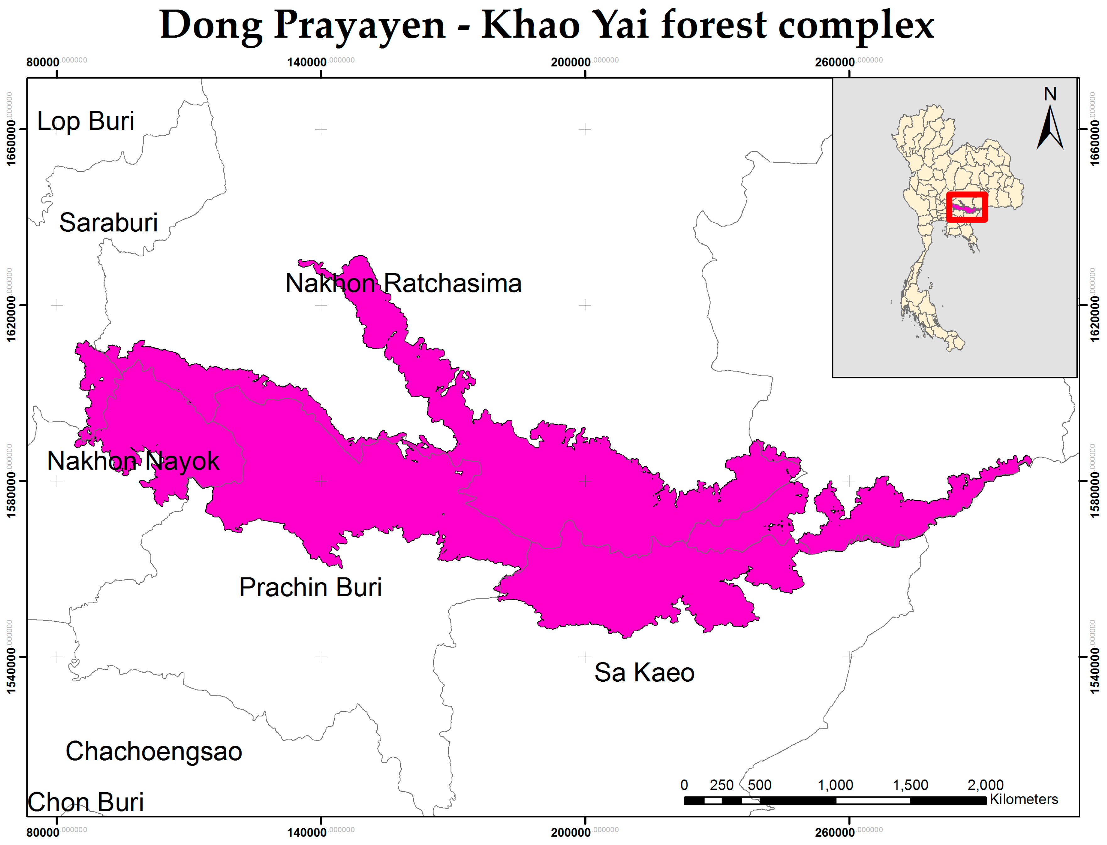
2.1. Study Area

The study area comprises the Dong Phayayen-Khao Yai Forest Complex, covering five protected areas from Khao Yai to the Cambodian border: Khao Yai National Park, Pang Sida National Park, Thap Lan National Park, Ta Phraya National Park, and Dong Yai Wildlife Sanctuary [38]. The region is an extension of the western part of the Sankamphang mountain range to the southwestern boundary of the Nakhon Ratchasima Province plateau (Figure 2). The majority of this site is located in Nakhon Ratchasima, but also extends across the Saraburi, Prachinburi and Nakhon Nayok Provinces of Thailand. The study area consists of a complex mountainous topography, including the peaks of Khao Rom, Khao Lam, Khao Keaw, Khao Sam Yod, Khao Far Pha, Khao Kampang, Khao Samor Poon and Khao Kaew, with elevations of 1351, 1326, 1292, 1142, 1078, 875, 805, and 802 meters above sea level, respectively [39]. Within this region, the most common forest types of Thailand occur, including both evergreen forests (EF) and deciduous forests (DF). As such, the complex topography and diverse forest ecosystem in this study area make it ideal for exploring topographic corrections of satellite imagery.

2.2. Landsat Imagery

The study dataset comprises Landsat TM-5 and OLI-8 images selected from the Land Processed Distributed Active Archive Centre (LP DAAC) (

Table 1. Specifications of Landsat Thematic Mapper-5 (TM) and Operational Land Imager-8 (OLI) imagery used in this study.

No	Landsat Sensor (Path/Row)	Date Acquired	Sun Azimuth	Sun Elevation
1	Landsat TM-5 128/050	1999-02-02	132.41329646	44.42900903
2	Landsat TM-5 129/050	1999-02-09	130. 01909034	45.70329359
3	Landsat OLI-8 128/050	2015-04-19	094. 94624942	65.59779841
4	Landsat OLI-8 129/050	2015-02-05	136.35602977	48.70124627

) [40]. Cloud-free images were chosen for this study, and only the red, green, blue, NIR, SWIR-1, and SWIR-2 bands of Landsat TM-5 and OLI-8 were included in the analysis. The image was converted to top-of-atmosphere (TOA) reflectance and atmospherically corrected using a dark pixel subtraction method [6]. Further, all images were adjusted using a forest normalization method, which uses the median value of evergreen forest to apply a linear shift to each spectral band [5,7].

2.3. Digital Elevation Models (DEM)

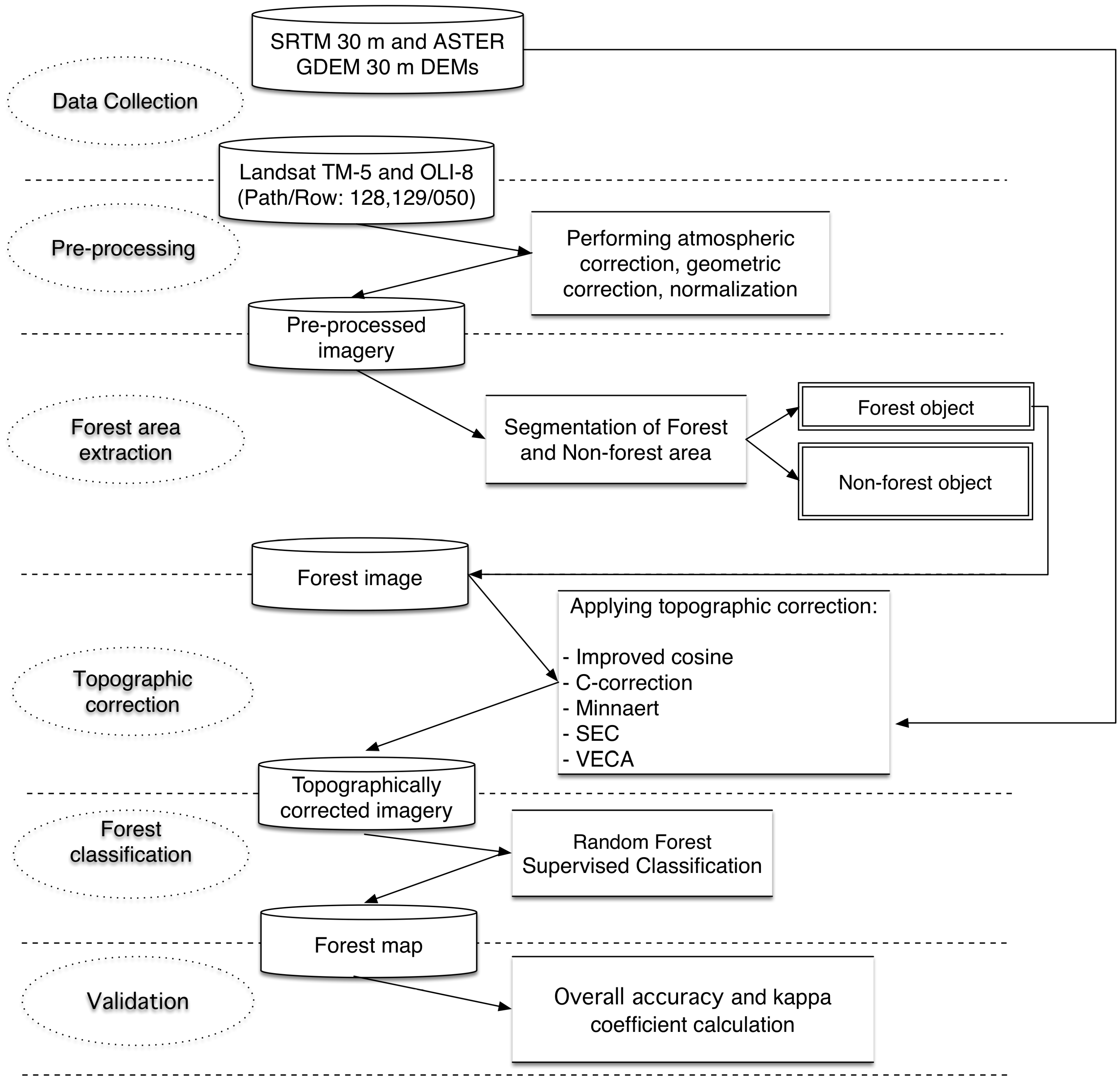
The DEMs used for topographic correction in this study were obtained from different sources. The National Aeronautics and Space Administration (NASA) SRTM 30 m ×30 m (1 arc-second) high-resolution DEM was obtained from the U.S. Geological Survey (USGS) [41] and resampled using a nearest neighborhood transformation [21].

Additionally, the ASTER GDEM has been generated from the stereoscopic ASTER satellite images. The ASTER GDEM, with 30 m × 30 m (1 arc-second) resolution, was downloaded from the USGS Earth Explorer platform [42] and resampled using a nearest neighborhood transformation [21]. The Japan Aerospace Exploration Agency’s Advance Land Observing Satellite “DAICHI” (ALOS) World 3D 30 m DEM was initially considered for this study, but due to the excessive number of missing tiles over the study area, it was not considered further for the analysis.

3. Methodology

This study consists of four major parts: topographic correction using multisource DEMs, evaluation of the topographic corrections, forest type classification, and an assessment of the effectiveness of the topographic correction on the overall accuracy of forest classifications. Figure 3 presents a flowchart that describes the process of Landsat imagery analysis, in addition to the topographic correction methods employed, the forest classification, and the evaluation of forest classification performance after the topographic correction procedure. Each step is discussed in detail below.

3.1. Stratification of Forest and Non-Forest Areas

Several studies have indicated that the application of topographic correction methods over large areas with different land cover types creates problems, resulting from specific LULC-dependent correction parameters such as the Minnaert factor and the C factor in a C-correction. On this basis, a number of studies have suggested that it is necessary to estimate the parameters separately for the individual LULC types that are present in the study area [5,26,27,43]. We therefore separate forest and non-forest areas, so that topographic correction can be performed on homogenous forest pixels based on actual reflectance values [5]. Firstly, forest and non-forest areas were distinguished using the object-oriented multi-resolution segmentation method [44]. The segmentation was performed based on Normalized Difference Vegetation Index (NDVI) calculated from red and NIR band of Landsat imagery using a scale factor of 90. Separation of forest and non-forest areas was performed within the eCognition software environment by training nearest neighbor classifier with approximately 100 training samples. Then, visual map refinement was performed to ensure high quality. The final segmented forest mask was then used to subset homogeneous forest area from Landsat image. It should be noted, however, that this segmentation does not allow for the complete separation of soil, bare land, and rocks inside and on the edge of the segmented forest object. To address this, we consider these pixels as non-forest throughout the analysis.

3.2. Topographic Correction Methods

Five different topographic correction methods were used on the stratified forest area (

Table 2. Summary of topographic correction methods used in this study on the DEM data.

No.	Correction Method	Equation
1	Improved cosine	${\mathsf{\rho }}_{\mathrm{H}}={\mathsf{\rho }}_{\mathrm{T}}+\left({\mathsf{\rho }}_{\mathrm{T}}\left(\frac{\overline{\mathrm{IL}}-\mathrm{IL}}{\overline{\mathrm{IL}}}\right) \right)$
2	C-correction	${\mathsf{\rho }}_{\mathrm{H}}={\mathsf{\rho }}_{\mathrm{T}}\left(\frac{\cos {\mathsf{\theta }}_{\mathrm{z}}+\mathrm{C}}{\mathrm{IL}+\mathrm{C}}\right)$
3	Minnaert	${\mathsf{\rho }}_{\mathrm{H}}={\mathsf{\rho }}_{\mathrm{T}}{\left(\frac{\cos {\mathsf{\theta }}_{\mathrm{z}}}{\mathrm{IL}}\right)}^{\mathrm{K}}$
4	Statistical-empirical	${\mathsf{\rho }}_{\mathrm{H}}={\mathsf{\rho }}_{\mathrm{T}}-\mathrm{ILm}-\mathrm{b}+\overline{{\mathsf{\rho }}_{\mathrm{T}}})$
5	VECA	${\mathsf{\rho }}_{\mathrm{H}}={\mathsf{\rho }}_{\mathrm{T}}+\frac{{\overline{\mathsf{\rho }}}_{\mathrm{T}}}{\left(\mathrm{mIL}+\mathrm{b}\right)}$

${\mathsf{\rho }}_{\mathrm{H}}$ = surface reflectance; ${\mathsf{\rho }}_{\mathrm{T}}$ = reflectance of an inclined surface; ${\mathsf{\theta }}_{\mathrm{z}}$ is the solar zenith angle; Illumination (IL); ${\mathsf{\theta }}_{\mathrm{p} }$ = slope angle; ${\varnothing }_{\mathrm{a} }$= solar azimuth angle; ${\varnothing }_{\mathrm{o}}$= aspect angle; $\overline{{\mathsf{\rho }}_{\mathrm{T}}}$ = mean of the radiance values of ${\mathsf{\rho }}_{\mathrm{T}}$ for tilted and horizontal surfaces of uncorrected forest pixels, and C and K are Minnaert constants.

). A detailed overview of the different topographic correction methods is shown in Figure 3. These are all based on the modeling of illumination (IL) conditions, and therefore require a DEM with the same spatial resolution as the Landsat TM-5 and OLI-8 imagery [26]. The IL conditions are then modeled using the ground slope and aspect with solar and satellite parameters [10,45]. A DEM is needed to compute the incident angle (${\gamma }_{і}$), defined as the angle between the normal to the ground and the sun’s rays [45]. The IL parameters lie between −1 and +1, indicating minimum and maximum illumination, respectively, and can be calculated using Equation (1):

$$\mathrm{IL}=\cos {\mathsf{\gamma }}_{\mathrm{i}}={\cos \mathsf{\theta }}_{\mathrm{p}}\cos {\mathsf{\theta }}_{\mathrm{z}}+\sin {\mathsf{\theta }}_{\mathrm{p}}\sin {\mathsf{\theta }}_{\mathrm{z}}\cos ({\varnothing }_{\mathrm{a}}-{\varnothing }_{\mathrm{o}})$$

(1)

where ${\mathsf{\theta }}_{\mathrm{p}}$ is the slope angle;${ \mathsf{\theta }}_{\mathrm{z}}$ is the solar zenith angle; ${\varnothing }_{\mathrm{a}}$ is the solar azimuth angle; and ${\varnothing }_{\mathrm{o}}$ is the aspect angle.

Once the IL is calculated, the obtained illumination can be used in Lambertian (improved cosine, C-correction), non-Lambertian (Minnaert), and empirical (SEC and VECA) topographic correction methods.

3.2.1. Improved Cosine Correction

The most commonly used Lambertian method is the cosine correction method, in which the reflectance of the surface is calculated using Equation (2):

$${\mathsf{\rho }}_{\mathrm{H}}={ \mathsf{\rho }}_{\mathrm{T}} \left(\frac{\cos {\mathsf{\theta }}_{\mathrm{z}}}{\mathrm{IL}}\right)$$

(2)

where ${\mathsf{\rho }}_{\mathrm{H}}$ is the surface reflectance; ${\mathsf{\rho }}_{\mathrm{T}}$ is the reflectance of an inclined surface; and ${\mathsf{\theta }}_{\mathrm{z}}$ is the solar zenith angle. This method does not require any external parameters. Several studies have shown that the cosine method tends to overcorrect in areas under low illumination conditions [10,19,26]. The improved cosine correction method was introduced by Civco in 1989 [22] to compensate for this overcorrection by the cosine method. In this, the average illumination ($\overline{\mathrm{IL}}$) is also included in the calculation (see Equation (3)) [26,45]. The $\overline{\mathrm{IL}}$ is average illumination across the stratified forest pixels in the image.

$${\mathsf{\rho }}_{\mathrm{H}}={ \mathsf{\rho }}_{\mathrm{T}}+ \left({\mathsf{\rho }}_{\mathrm{T}}\left(\frac{\overline{\mathrm{IL}}-\mathrm{IL}}{\overline{\mathrm{IL}}}\right) \right)$$

(3)

3.2.2. C-Correction

The improved cosine correction is a wavelength independent method. Teillet et al. [19] proposed the C-correction method, which considers the difference between bands under diffuse irradiation. As such, the C-correction method is a band-specific regression coefficient topographic correction method, which incorporates a modified cosine correction parameter, C. Based on the linear relationship between IL and reflectance data, the empirical constant (C) can be automatically calculated for each band of Landsat TM-5 and OLI-8 data (see Equation (4)) [8,26,46].

$${\mathsf{\rho }}_{\mathrm{H}}={ \mathsf{\rho }}_{\mathrm{T}} \left(\frac{\cos {\mathsf{\theta }}_{\mathrm{z}}+\mathrm{C}}{\mathrm{IL}+\mathrm{C}}\right)$$

(4)

where ${\mathsf{\rho }}_{\mathrm{T}}$ is the reflectance of an inclined surface and can be calculated as ${\mathsf{\rho }}_{\mathrm{T}}=\mathrm{b}+\mathrm{mIL}$; C is an empirical constant that is calculated using $\mathrm{C}=\frac{\mathrm{b}}{\mathrm{m} }$; and b and m are the regression coefficients between the illumination and the different band reflectances.

3.2.3. Minnaert Correction

The non-Lambertian methods assume that the combination of the angles of incidence and observation can affect reflectance, and that surface roughness is also an important factor. One of the most widely used methods for forest studies is the Minnaert correction, proposed by Minnaert in 1941 [1,10,26,47]. This method adds a band-specific constant (K) to the cosine correction method (see Equation (5)) [10,45]. It is assumed that if the Minnaert constant (K) is 1, the surfaces behave in a perfectly Lambertian manner and the Minnaert values and cosines are equivalent [1,10,45]. In this study, the Minnaert constant (K) was calculated automatically for forest and non-forest areas [5].

$${\mathsf{\rho }}_{\mathrm{H}}={ \mathsf{\rho }}_{\mathrm{T}} {\left(\frac{\cos {\mathsf{\theta }}_{\mathrm{z}}}{\mathrm{IL}}\right)}^{\mathrm{K}}$$

(5)

where the K band-specific constant; and K and $\ln ({\rho }_H)$ are the regression coefficients. That is, ${\mathsf{\rho }}_{\mathrm{H}}$ is constant across the entire image for each band [10] (see Equation (6)).

$$\ln ({\mathsf{\rho }}_{\mathrm{T}})=\ln ({\mathsf{\rho }}_{\mathrm{H}})+\mathrm{K}\ln (\frac{\mathrm{IL}}{\cos {\mathsf{\theta }}_{\mathrm{z}} })$$

(6)

3.2.4. Statistical Empirical Correction (SEC)

The empirical correction methods are based on the relationship between radiance and the angle of incidence [21,36]. The SEC correlates the pixel reflectance values with the corresponding predicted IL from the DEM, and the slope of the regression line defines the statistical relationship between a given forest and the variation of its radiometric response as a function of terrain slope [48]. This method is land use specific (usually forest) [49]. The presence of non-forest outliers in the regression between radiance and incidence angle might alter the sensibly of the equation [48].

$${\mathsf{\rho }}_{\mathrm{H}}={\mathsf{\rho }}_{\mathrm{T}}-\mathrm{mIL}-\mathrm{b}+\overline{{\mathsf{\rho }}_{\mathrm{T}}}$$

(7)

where m is the slope of the regression line, b is the y-intercept of the regression line, and $\overline{{\mathsf{\rho }}_{\mathrm{T}}}$ is the mean of the ${\mathsf{\rho }}_{\mathrm{T}}$ radiance values for uncorrected forest pixels on tilted and horizontal surfaces [31,49].

3.2.5. Variable Empirical Coefficient Algorithm (VECA)

The VECA method was proposed by Gao and Zhang, 2009 [31], and is based on the theoretical and statistical analysis of the radiance values (see Equation (8)).

$${\mathsf{\rho }}_{\mathrm{H}}={\mathsf{\rho }}_{\mathrm{T}}\frac{{\overline{\mathsf{\rho }}}_{\mathrm{T}}}{\left(\mathrm{mIL}+\mathrm{b}\right)}$$

(8)

$$\mathsf{\lambda }=\frac{{\overline{\mathsf{\rho }}}_{\mathrm{T}}}{\left(\mathrm{mIL}+\mathrm{b}\right)}$$

(9)

where $\mathsf{\lambda }$ is called an adjustment factor. Equation (8) can be written as Equation (10), in which$\mathsf{\lambda }$ is directly proportional to ${\mathsf{\rho }}_{\mathrm{T}}$ [30].

$${\mathsf{\rho }}_{\mathrm{H}}={\mathsf{\rho }}_{\mathrm{T}}\mathsf{\lambda }$$

(10)

The main aim of all of these topographic corrections is to reduce the variations in incident radiation introduced by solar illumination of uneven mountainous terrain, affecting the same forest cover located on opposite sides of a mountain or in its shadows. Topographic corrections in mountainous forest cover type should produce the same reflectance at different solar azimuths, and so will show the same spectral response in remotely sensed imagery [30].

3.3. Evaluation of Topographic Correction Methods

The performances of the topographic correction methods were evaluated by comparing topographically corrected and uncorrected Landsat TM-5 and OLI-8 imagery, using visual interpretation and statistical assessment based on the multisource DEMs.

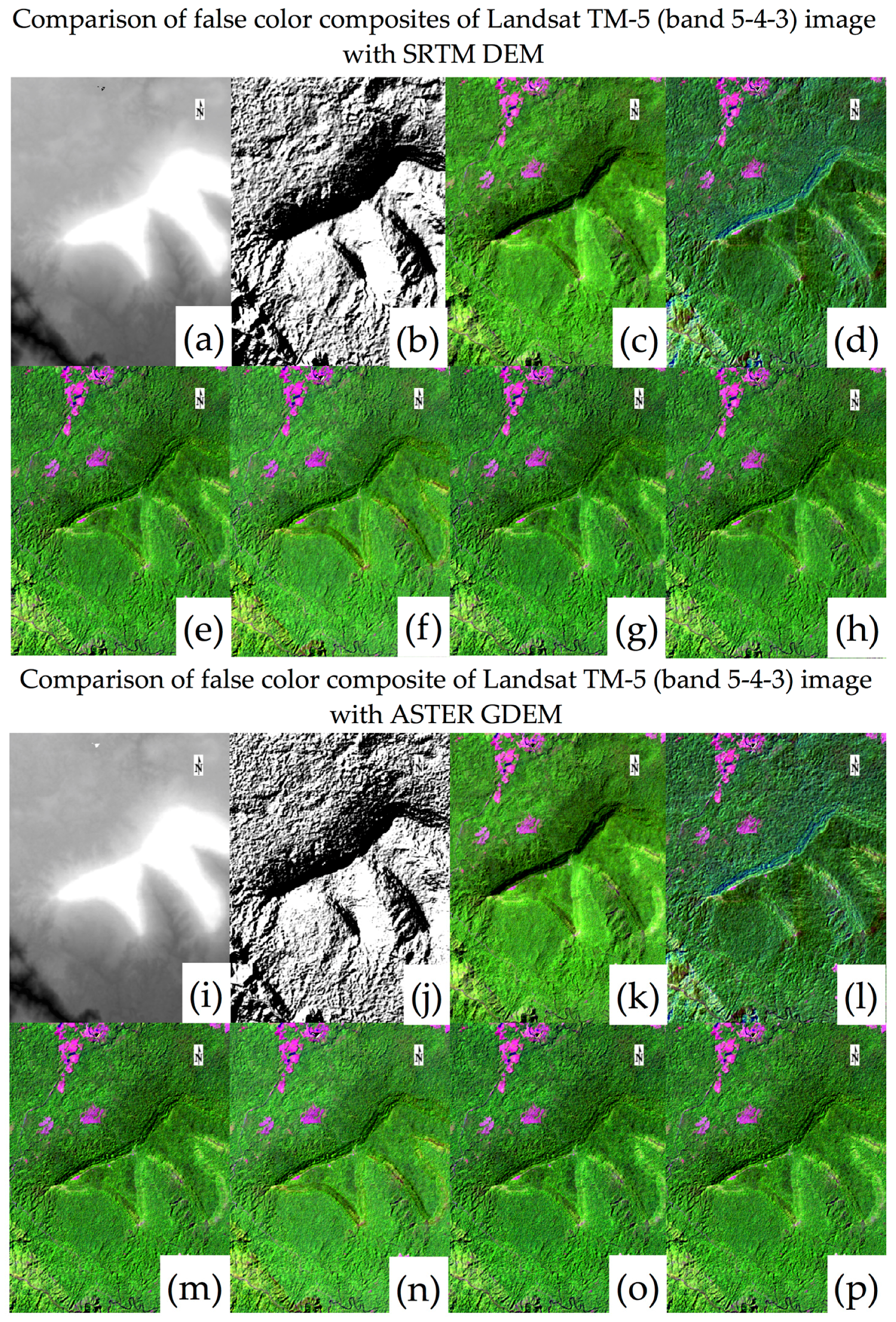
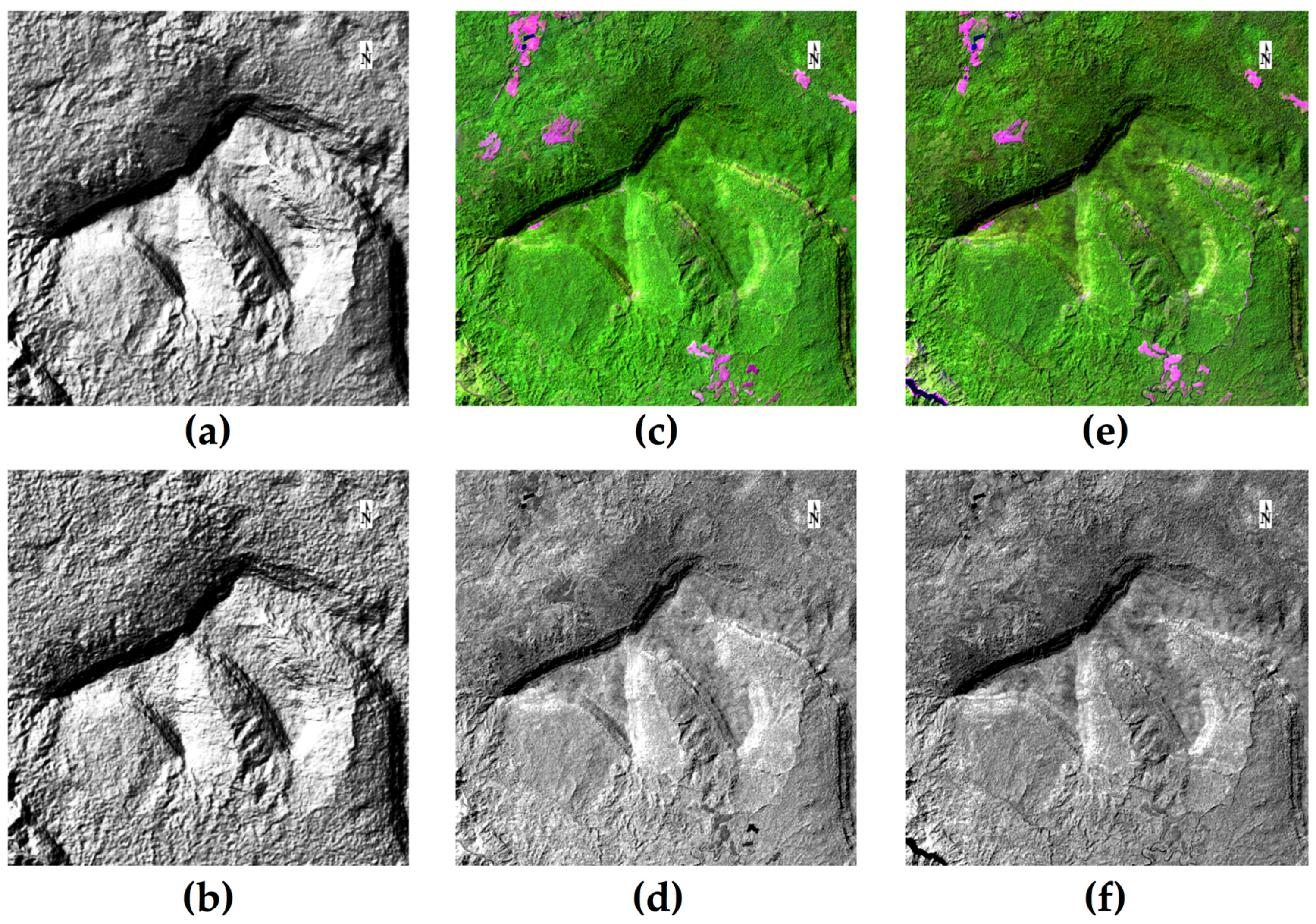
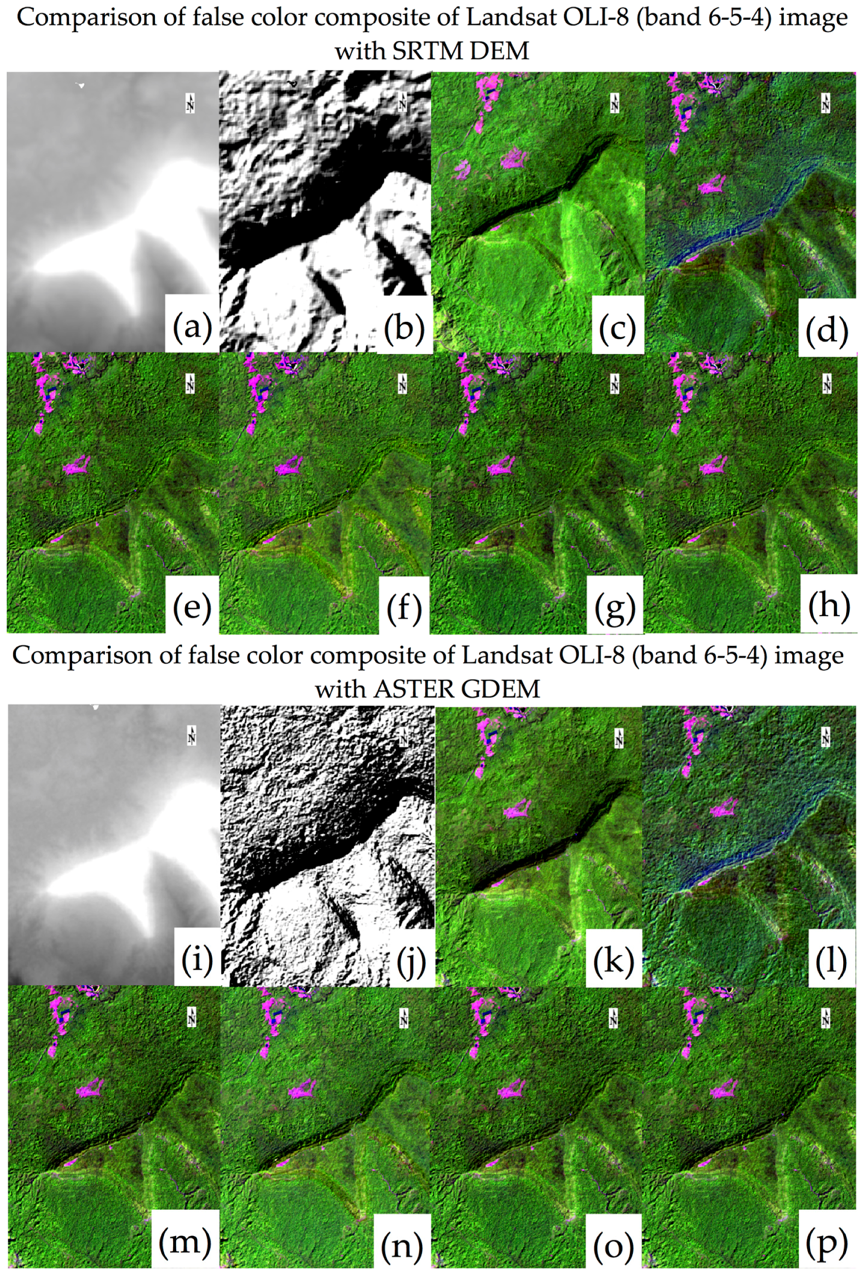
3.3.1. Visual Interpretation

Firstly, the quality of topographic correction was assessed by visual interpretation of corrected and uncorrected imagery. The visual assessment of uncorrected and corrected images gives an indication of the correction effect. In most of the cases, noticeable or minor differences could be observed in the true color, false color, and pseudo natural color composites. However, the interpretation of results depends heavily on the skill of the image analyst or observer. In order to obtain a better understanding, the visual evaluation of corrected imagery must be combined with a quantitative statistical assessment [21,28,29].

3.3.2. Statistical Interpretation

The performances of the topographic corrections were further examined using mean and standard deviation (SD) of individual Landsat TM-5 and OLI-8 bands. The correction methods were evaluated based on analyses that test the homogeneity of reflectance values within a given forest area. Spectral characteristics of the selected forest pixels before and after the correction were extracted and compared. A successful correction should decrease the variability (SD) within each band, while the mean value of each image band should be very close to each other [10]. The relative variability (SD) should show a reduction compared to the uncorrected image bands. This change in SD value indicates the removal of topographic shadow effects. The quality of topographic correction can therefore be estimated using the relative variability of reflectance within each forest type. In previous works, the reduction of the SD of the reflectance from the forest cover was calculated by the coefficient of variation (CV) [9,15,17,21,28,33]. The CV is simply the ratio of the SD to the mean reflectance, expressed as a percentage (Equation (11)).

$$\mathrm{CV}(\%)=\frac{\mathrm{SD}}{\mathsf{\mu } }\times 100 .$$

(11)

where CV is the coefficient of variance for reflectance values of selected forest pixels, SD is the standard deviation of reflectance values, and $\mathsf{\mu }$ is the mean of the reflectance values. The CV is expected to decrease after a successful topographic correction. For a better evaluation of the changes before and after correction, CV values of all bands and the CV differences were calculated using Equation (12) [33]. In this, positive values of CV_Difference indicate a decrease in CV.

$${\mathrm{CV}}_{\mathrm{Difference}}={\mathrm{CV}}_{\mathrm{Before}-\mathrm{correction}}-{\mathrm{CV}}_{\mathrm{After}-\mathrm{correction}}$$

(12)

3.3.3. Evaluation of Shadow and Non-Shadow Area

The most suitable DEM and best performing correction methods were selected based on ${\mathrm{CV}}_{\mathrm{Difference}}$ values (see Section 3.2.2). In order to evaluate performance of a topographic correction method in shadow and non-shadow areas, the reflectance values of uncorrected and corrected images in both areas were compared. The average and CV for each band of Landsat TM-5 and OLI-8 uncorrected and corrected images were compared. The best method should decrease the variability within each band of the shadow areas, while the average value of each image band should be increased. On the other hand, in the non-shadow areas, the average and CV should not vary from the uncorrected image reflectance. This behavior of reflectance in shadow and non-shadow areas indicates that the best topographic correction has only been applied on topographic shadows, while preserving the original reflectance values of the image [31].

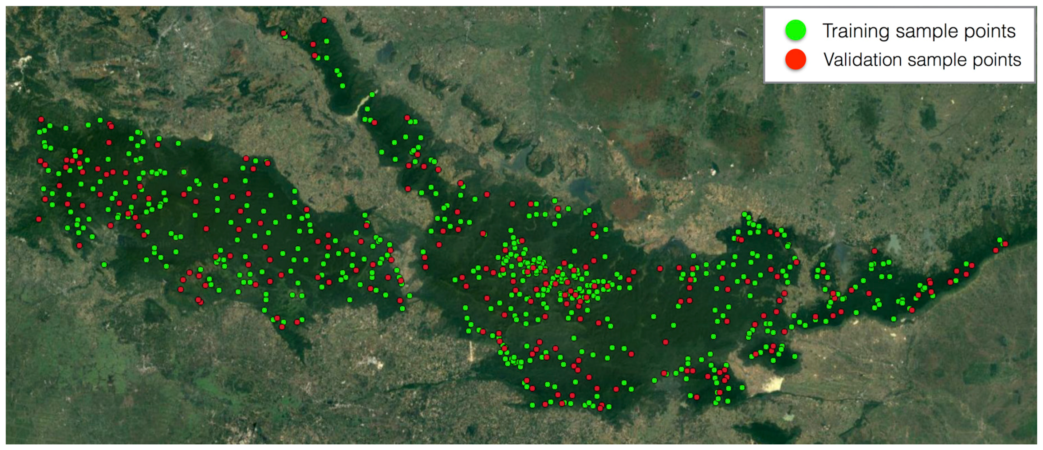
3.4. Training and Validation Data

The selection of a systematic training and validation dataset across a forest landscape ensures a sample that has the proportions of the forest classes, and which represents the actual area occupied by different forest types. It must be assumed that the sample should be a good representative of forest pixels, and is sufficiently large to provide reliable estimates. For the present study, we used a stratified random sampling approach to estimate the total sample size per class [50,51]. In total, 767 sample locations were selected for all forest and non-forest classes. Among these, 667 locations were collected for the three major forest types: Class 1, Evergreen forest (EF); Class 2, Deciduous forest (DF); and Class 3, Bamboo forest (BB). For the non-forest (NF) Class 4, around one hundred sample locations were created, using the existing land use map and interpretations of the high-resolution imagery. For each forest type, the numbers of training sample points were: 237 for EF; 108 for DF; 100 for BF; and 70 for NF. We manually collected many training and validation samples, 152 of which were from a field survey conducted in March, 2015, and around 100 were derived from previous field surveys by the Royal Forest Department, Thailand during 2008 and 2009. We have carefully selected these forest locations to ensure that the sample is taken from an undisturbed forest area. The dominant forest type and topographic data, such as slope, elevation, and forest conditions, was recorded for each individual sample location. A combination of Google Earth images, high-resolution satellite imagery, aerial photographs, and prior knowledge were used to sample the remaining locations in remote areas that were difficult or impossible to access. Among these sample locations, 252 were randomly selected to be set aside as validation data samples, and to avoid spatial autocorrelation, the selected training and validation pixels were chosen to not be close to one another [32]. The size of training sample for each class was greater than 50 pixels (Figure 4).

3.5. Forest Classification

Prior to forest classification, the satellite imagery was pre-processed and topographically corrected. Pre-processing incorporates atmospheric correction, geometric correction, image normalization, topographic correction, the segmentation of forest and non-forest areas, and construction of a mosaic of Landsat images for path/row: 128/50 and 129/50. The performance of each topographic correction method was tested against the SRTM DEM and ASTER GDEM, and the topographic correction method that performs the worst with both DEMs is not considered in further classifications. We performed a series of supervised pixel-based classifications of topographically uncorrected and corrected imagery with the RF classifier. The classification scheme included the four classes mentioned in Section 3.4: Class 1, EF; Class 2, DF; Class 3, BF; and Class 4, NF. It should be noted that the same training and testing data samples were used for the supervised classification of the corrected and uncorrected imagery. A 3 × 3 majority filter was applied to the classified imagery to remove salt-and-pepper effects and to minimize the omission errors [52].

Random Forest (RF) Classifier

The RF classifier was used for forest classification [53,54]. It is a widely used non-parametric machine learning classifier consisting of an ensemble of decision trees and bootstrapping with replacements [55,56]. RF is based on a tree classifier and grows many classification trees. In order to classify a new vector, the input vector is classified alongside each of the trees in the forest. Each tree gives a classification, and the tree votes for that class. The forest then chooses the classification with maximum votes from all of the classification trees in the forest [57]. The advantages of using RF is its potential to determine the importance of variables, its robustness to data reduction, no tendency to over fit, the production of an unbiased accuracy estimate, and a higher accuracy than decision trees with lower sensitivity to tuning parameters [58].

In this study, we used the RF implementation in R packages Random Forest [53,54,59] and RStoolbox [60], as well as the Quantum GIS open source GIS software package [61].

3.6. Accuracy Assessment

During the classification process, around 70% of the sample points were used to train the classifier, while the remaining 30% of sample points used to test the accuracy and validate the classifier (Figure 4). The accuracies of the RF classifier were considered through assessments of the overall accuracy and Kappa statistics (KHAT) [11,17,55,62]. In this study, the kappa coefficients of Landsat TM-5 and OLI-8 imagery are derived as a second measure of classification accuracy. The Kappa values indicate a fair level of agreement between the RF classifier prediction of forest class and the actual field survey data [18]. The accuracy of classified topographically uncorrected imagery was assessed and compared with the following scenario: RF with four classes—classified topographically corrected imagery using the SRTM DEM.

4. Results

4.1. Evaluation of Topographic Correction Methods

The performances all topographic correction algorithms were evaluated by comparing topographically corrected and uncorrected Landsat TM-5 and OLI-8 images, using visual interpretation and statistical assessment based on the two DEMs (SRTM and ASTER GDEM).

4.1.1. Visual Interpretation with SRTM and ASTER GDEM Based Topographic Correction

Figure 5 and Figure 6 show false color composites (Landsat TM-5: Band 5-4-2 and Landsat OLI-8: band 6-5-4) of selected sites in the study area, both uncorrected and topographically corrected using the SRTM DEM and ASTER GDEM. The illumination (Figure 5b,j) shows the cosine of the solar incident angle calculated using these DEMs. Figure 5b,j and Figure 6b,j clearly show that those forest areas facing the Sun receive more light and appear brighter, while forest areas in the mountain shadows appear darker. The uncorrected Landsat TM-5 and OLI-8 images also reveal the visible effect of topographic shadows. A comparison of the topographically uncorrected and corrected imagery shows the significant effect of mountain shadows on reflectance values (Figure 5 and Figure 6). After topographic correction, however, a significant reduction in the topographic relief effect have been observed. The Landsat TM-5 and OLI-8 images show noticeable differences after correction with both the SRTM DEM and ASTER GDEM, especially in those areas that are shaded by steep slopes (Figure 5 and Figure 6).

The C-correction, Minnaert, SEC and VECA topographic corrections all seem to show a greater reduction in the topographic effect than the improved cosine correction. The selected site pictured in Figure 5 and Figure 6 has an extremely uneven mountain topography covered mainly by evergreen forest. The improved cosine correction shows a small overcorrection in Figure 5d,l, and Figure 6d,l, which is caused by the Lambertian reflectance assumptions. Many studies have reported similar behavior in the cosine correction method [10,13,14,63]. Among the five methods investigated here, the C-correction, SEC, and VECA appear to perform the best, because their corrected images are more homogenous and have a darker appearance than the images produced by other topographic correction methods. The overcorrection of the improved cosine correction is not apparent in any of the other corrected images. Additionally, it should be noted that in the very dark shadows the SRTM DEM produces a greater decrease in the relief effect than the ASTER GDEM. All of the topographic correction methods were capable of producing an image in which all the pixels of the same forest type appeared the same, regardless of terrain slope and mountain shadows.

4.1.2. Statistical Interpretation of SRTM DEM and ASTER GDEM-Based Topographic Corrections

A coarse classification of the Landsat OLI-8 data from 2015 is conducted, based on SEC corrected imagery employing the four major classes mentioned in Section 3.4 [28]. We applied this coarse classification to maintain homogeneity when selecting the forest pixels, so that the performance of topographic corrections can be evaluated with respect to individual forest types.

Table 3. CVs and CV differences in the reflectances of forest types in topographically uncorrected and corrected Landsat TM-5 images, based on the: (a) SRTM DEM; and (b) ASTER GDEM. Class 1: Evergreen forest (EF), Class 2: Deciduous forest (DF), Class 3: Bamboo forest (BF).

(a) Landsat TM-5 Using STRM DEM
	Original			Improved Cosine			C-Correction			Minnaert			SEC			VECA
CV	Evergreen Forest	Deciduous Forest	Bamboo Forest	Evergreen Forest	Deciduous Forest	Bamboo Forest	Evergreen Forest	Deciduous Forest	Bamboo Forest	Evergreen Forest	Deciduous Forest	Bamboo Forest	Evergreen Forest	Deciduous Forest	Bamboo Forest	Evergreen Forest	Deciduous Forest	Bamboo Forest
Band 1	2.85	3.55	2.10	12.91	26.87	25.93	2.59	3.23	3.92	8.73	4.31	3.66	2.50	3.23	3.61	2.59	3.23	4.05
Band 2	7.11	8.99	5.40	11.54	24.05	23.67	5.78	7.36	4.63	9.81	7.67	4.71	5.21	7.50	4.86	5.78	7.36	4.78
Band 3	7.37	13.75	8.05	12.12	22.97	22.50	6.17	11.71	6.25	9.48	11.84	5.97	5.56	12.07	5.87	6.17	11.71	6.42
Band 4	21.18	18.98	15.34	13.43	26.15	20.76	14.02	17.77	12.37	14.94	17.28	11.80	9.95	19.07	10.91	14.02	17.77	12.35
Band 5	26.66	34.18	26.94	17.49	26.10	18.66	18.35	26.83	18.21	19.39	27.35	17.92	11.74	28.35	16.75	18.35	26.83	18.33
Band 6	30.38	44.20	31.51	24.14	30.14	20.81	24.76	35.78	22.31	25.54	36.69	22.01	15.90	38.20	19.71	24.76	35.78	22.50
Average	15.93	20.61	14.89	15.27	26.05	22.06	11.94	17.11	11.28	14.65	17.52	11.01	8.48	18.07	10.28	11.94	17.11	11.40
Difference of average CVs	-	-	-	0.65	−5.43	−7.16	3.98	3.49	3.60	1.27	−2.63	3.87	7.44	2.54	4.60	3.98	3.49	3.48
(b) Landsat TM-5 Using ASTER GDEM
	Original			Improved Cosine			C-Correction			Minnaert			SEC			VECA
CV	Evergreen Forest	Deciduous Forest	Bamboo Forest	Evergreen Forest	Deciduous Forest	Bamboo Forest	Evergreen Forest	Deciduous Forest	Bamboo Forest	Evergreen Forest	Deciduous Forest	Bamboo Forest	Evergreen Forest	Deciduous Forest	Bamboo Forest	Evergreen Forest	Deciduous Forest	Bamboo Forest
Band 1	2.85	3.55	2.10	15.08	23.71	26.26	2.64	3.24	3.41	9.09	4.00	4.09	2.55	3.24	3.83	2.64	3.24	3.58
Band 2	7.11	8.99	5.40	14.21	20.72	24.11	6.18	7.36	4.46	9.76	7.11	5.13	5.67	7.50	4.76	6.18	7.36	4.64
Band 3	7.37	13.75	8.05	14.65	19.92	23.23	6.59	11.77	6.41	9.39	11.00	6.40	6.10	12.11	6.67	6.59	11.77	6.63
Band 4	21.18	18.98	15.34	16.68	23.75	19.91	16.89	16.96	11.43	20.33	16.65	11.23	12.59	17.90	10.78	16.89	16.96	11.40
Band 5	26.66	34.18	26.94	20.46	25.19	19.41	21.19	27.49	19.22	24.14	27.55	19.02	14.86	28.59	20.02	21.19	27.49	19.39
Band 6	30.38	44.20	31.51	26.69	30.39	21.93	26.89	36.77	23.63	28.27	36.84	23.36	18.80	38.85	25.41	26.89	36.77	23.90
Average	15.93	20.61	14.89	17.96	23.95	22.47	13.40	17.26	11.43	16.83	17.19	11.54	10.09	18.03	11.91	13.40	17.26	11.59
Difference of average CVs	-	-	-	−2.03	−3.33	−7.58	2.52	3.34	3.46	−0.90	3.41	3.35	5.83	2.57	2.97	2.52	3.34	3.30

and

Table 4. CVs and CV differences in the reflectances of forest types in topographically uncorrected and corrected Landsat OLI-8 images, based on the: (a) SRTM DEM; and (b) ASTER GDEM. Class 1: Evergreen forest (EF), Class 2: Deciduous forest (DF), Class 3: Bamboo forest (BF).

(a) Landsat OLI-8 Using SRTM DEM
	Original			Improved Cosine			C-Correction			Minnaert			SEC			VECA
CV	Evergreen Forest	Deciduous Forest	Bamboo Forest	Evergreen Forest	Deciduous Forest	Bamboo Forest	Evergreen Forest	Deciduous Forest	Bamboo Forest	Evergreen Forest	Deciduous Forest	Bamboo Forest	Evergreen Forest	Deciduous Forest	Bamboo Forest	Evergreen Forest	Deciduous Forest	Bamboo Forest
Band 2	1.95	3.08	2.43	12.11	23.02	10.52	1.40	2.57	3.56	8.29	3.84	3.87	1.34	2.58	3.86	1.40	2.57	3.70
Band 3	6.14	8.94	7.72	10.03	20.22	10.04	4.09	7.13	6.67	8.47	7.53	7.25	3.67	7.22	6.70	4.09	7.13	6.72
Band 4	7.16	14.73	10.58	10.14	18.52	11.90	5.25	12.57	9.57	9.70	12.81	10.08	4.72	12.80	9.95	5.25	12.57	9.66
Band 5	22.21	21.78	9.49	13.49	22.75	8.88	14.29	18.53	7.39	15.20	18.44	7.12	9.75	19.02	7.37	14.29	18.53	7.52
Band 6	25.06	32.40	13.84	17.55	23.84	11.40	18.21	25.62	11.10	19.06	26.10	11.52	12.44	26.55	11.30	18.21	25.62	11.20
Band 7	24.66	36.98	15.64	18.47	25.74	13.14	19.11	29.98	13.14	20.07	30.61	13.88	13.43	31.22	13.64	19.11	29.98	13.27
Average	14.53	19.65	9.95	13.63	22.35	10.98	10.39	16.07	8.57	13.46	16.56	8.95	7.56	16.57	8.80	10.39	16.07	8.68
Difference of average CVs	-	-	-	0.89	−2.69	−1.02	4.13	3.58	1.38	1.06	3.09	0.99	6.97	3.08	1.14	4.13	3.58	1.27
(b) Landsat OLI-8 Using ASTER GDEM
	Original			Improved Cosine			C-Correction			Minnaert			SEC			VECA
CV	Evergreen Forest	Deciduous Forest	Bamboo Forest	Evergreen Forest	Deciduous Forest	Bamboo Forest	Evergreen Forest	Deciduous Forest	Bamboo Forest	Evergreen Forest	Deciduous Forest	Bamboo Forest	Evergreen Forest	Deciduous Forest	Bamboo Forest	Evergreen Forest	Deciduous Forest	Bamboo Forest
Band 2	1.95	3.08	2.43	14.13	20.03	10.92	1.56	2.63	3.24	8.66	3.62	4.44	1.51	2.64	3.54	1.56	2.63	3.42
Band 3	6.14	8.94	7.72	12.85	17.60	10.56	4.87	7.39	6.79	8.49	7.15	7.56	4.50	7.45	6.85	4.87	7.39	6.85
Band 4	7.16	14.73	10.58	13.12	16.56	12.09	5.98	12.91	9.59	9.51	11.91	10.16	5.51	13.10	9.99	5.98	12.91	9.68
Band 5	22.21	21.78	9.49	16.47	21.67	9.85	17.04	18.79	7.87	19.04	18.71	7.84	12.53	19.11	7.86	17.04	18.79	7.99
Band 6	25.06	32.40	13.84	20.14	24.51	11.99	20.62	26.89	11.55	22.18	26.83	12.00	15.03	27.55	11.79	20.62	26.89	11.66
Band 7	24.66	36.98	15.64	21.03	26.94	13.66	21.15	31.29	13.56	22.42	31.18	14.32	15.73	32.28	14.10	21.15	31.29	13.70
Average	14.53	19.65	9.95	16.29	21.22	11.51	11.87	16.65	8.77	15.05	16.57	9.39	9.14	17.02	9.02	11.87	16.65	8.88
Difference of average CVs	-	-	-	−1.76	−1.56	−1.55	2.65	3.00	1.18	−0.52	3.08	0.56	5.39	2.62	0.93	2.65	3.00	1.06

show the selected homogenous forest pixels for each forest type and each band of the Landsat TM-5 and OLI-8 data. The number and locations of pixels used to calculate the CV from each band of the image are the same. Furthermore, Table 3 and Table 4 also show the mean CV and CV_Difference values for the selected pixels in the corrected and uncorrected spectral bands of the Landsat TM-5 and OLI-8 data. The results after topographic correction show the effectiveness of the topographic correction methods. The difference between the results from the two DEMs can be evaluated using the average CV_Difference values (Table 3 and Table 4), which indicated that the CV values were lowered compared with the uncorrected imagery. However, in most cases, the SRTM DEM better maintained the mean and reduced CV, compared to the ASTER GDEM. The positive CV_Diffrence values in most of these cases indicate an increase in performance.

The improved cosine correction method shows lower CV_Difference values than the other topographic correction methods for all three forest types: EF, DF, and BF. It can be seen from Figure 5 and Figure 6 and Table 3 and 4 that the improved cosine correction appears to be able to reduce the topographic relief effect but results in lower CV_Difference values. In contrast, after correction by SEC, VECA, and C-correction, the CV_Difference values are increased dramatically compared with the uncorrected imagery, indicating that there is no overcorrection by these methods.

Table 3 presents the changes in the reflectance characteristics of the Landsat TM-5 images, corrected using the SRTM DEM and ASTER GDEM in the study area. With the SRTM DEM, SEC ranks highest overall, with the greatest CV_Difference values for EF, DF, and BF of 7.44, 2.54, and 4.60, respectively. A reduction in CV values can be observed in the vegetation-sensitive bands such as NIR and SWIR, and in individual forest classes. The improved cosine and Minnaert correction methods resulted in a decrease in CV_Difference values. Thus, SEC ranks first, followed by VECA, the C-correction, Minnaert and the improved cosine correction (Table 3a). Additionally, the CV_Difference values presented here for the SEC correction are higher for EF than for DF and BF, because the mean reflectance values are lower for EF after correction, especially in the NIR and SWIR spectral bands.

Table 3b shows the CV and CV_Difference values for the Landsat TM-5 imagery topographically corrected using the ASTER GDEM. Results for EF, DF, and BF reveal that almost all of the methods are able to increase the CV_Difference values, with the exception of the improved cosine and Minnaert corrections. It can be seen that the results with the ASTER GDEM are little more inconsistent than with the previous DEM. For EF, SEC is able to increase the CV_Difference values better than the other methods, whereas the C-correction, Minnaert, and VECA increase the CV_Difference values for DF and BF more than the SEC correction. Moreover, the comparison between multisource DEMs reveals that the SRTM DEM-corrected Landsat TM-5 imagery is able to maintain a higher rate of CV_Difference values than that corrected with the ASTER GDEM.

Table 4 presents the reflectance values of the Landsat OLI-8 data, corrected using the SRTM DEM and ASTER GDEM in the study area. With the SRTM DEM, SEC produces an increase in CV_Difference values in EF, while the C-correction, VECA and Minnaert are better able to maintain CV_Difference values in the DF and BF classes, compared to SEC (Table 4a). It should be noted that EF occupies the majority of the study area, and is located particularly in regions with uneven mountainous terrain. In contrast, DF and BF together occupy a smaller area than the EF, and tend to be located in less sloping and flatter terrain. The corrections utilizing the ASTER GDEM follow similar trends, and are able to maintain higher CV_Difference values, with the exception of the improved cosine and Minnaert corrections.

The results presented here indicate that most of the topographic correction methods produce an increase in CV_Difference values. However, the obtained CV_Difference values are highly influenced by the DEM used for the topographic correction, such that the SRTM DEM-based SEC of Landsat TM-5 resulted in higher CV_Difference values than with the ASTER DEM (Table 3). Decreases in CV_Difference values are rarely observed with the SRTM DEM-based topographic corrections, and are slightly more common with the ASTER GDEM. An overall comparison of CV_Difference values for different topographic correction methods suggests that the SEC method performs best, followed by VECA and the C-correction, while the improved cosine and Minnaert corrections perform the worst, especially with the ASTER GDEM. Consequently, the SRTM DEM-based SEC, VECA and C-correction imagery are used for subsequent classifications, with the uncorrected imagery for comparison.

4.2. Performance Evaluation of Topographic Correction Methods in Shadow and Non-Shadow Area

From the previous analysis, we can state that the SRTM DEM produced slightly better results than the ASTER GDEM. In this section, we used only SRTM DEM based topographically corrected images to identify the best performing method in topographic shadow and non-shadow areas. In the above results, the improved cosine and Minnaert correction methods performed the worst on the SRTM DEM, so we only used the SEC, VECA, and C-corrected images for comparing shadow and non-shadow areas. Mean reflectance and CV values of the selected homogeneous shadow and non-shadow test pixels for each band of Landsat TM-5 and OLI-8 (uncorrected and corrected) were calculated and presented in

Table 5. Comparison of Landsat TM-5 reflectance in shadow and non-shadow area (unit percentage).

Shadow Area (a)	Original		C-Correction		SEC		VECA
Statistics	Average	CV	Average	CV	Average	CV	Average	CV
Band 1	7.43	2.26	7.58	2.21	7.69	2.13	7.67	2.21
Band 2	4.77	5.61	5.25	5.66	5.40	5.03	5.28	5.66
Band 3	3.16	6.05	3.53	5.74	3.66	4.88	3.55	5.74
Band 4	10.59	20.62	16.44	20.00	18.16	11.50	16.18	20.00
Band 5	3.90	23.77	6.14	22.99	7.39	11.72	6.04	22.99
Band 6	1.51	30.31	2.28	29.16	2.84	14.76	2.24	29.16
Average		14.77		14.29		8.34		14.29
Difference of average CV		-		0.48		6.43		0.48
Non-Shadow Area (b)	Original		C-Correction		SEC		VECA
Statistics	Average	CV	Average	CV	Average	CV	Average	CV
Band 1	7.84	2.63	7.86	2.65	7.95	2.61	7.95	2.65
Band 2	5.91	3.70	5.98	3.84	6.02	3.78	6.01	3.84
Band 3	3.91	5.82	3.97	5.75	4.00	5.62	3.99	5.75
Band 4	19.40	4.30	20.41	5.37	20.14	5.21	20.09	5.37
Band 5	7.63	5.47	8.04	6.44	7.96	6.43	7.90	6.44
Band 6	2.79	9.32	2.93	10.29	2.92	10.16	2.88	10.29
Average		5.21		5.72		5.64		5.72
Difference of average CV		-		−0.51		−0.43		−0.51

and

Table 6. Comparison of Landsat OLI-8 reflectance in shadow and non-shadow area (unit percentage).

Shadow Area (a)	Original		C-Correction		SEC		VECA
Statistics	Average	CV	Average	CV	Average	CV	Average	CV
Band 1	7.55	1.31	7.75	1.24	7.86	1.18	7.84	1.24
Band 2	5.12	4.29	5.74	4.01	5.85	3.48	5.76	4.01
Band 3	3.18	5.13	3.55	4.91	3.65	4.24	3.57	4.91
Band 4	12.50	21.42	19.12	20.83	21.18	12.01	18.82	20.83
Band 5	4.98	24.49	7.65	23.74	8.72	13.08	7.52	23.74
Band 6	2.08	24.34	3.06	23.69	3.47	13.79	3.02	23.69
Average		13.50		13.07		7.96		13.07
Difference of average CV		-		0.43		5.54		0.43
Non-Shadow Area (b)	Original		C-Correction		SEC		VECA
Statistics	Average	CV	Average	CV	Average	CV	Average	CV
Band 1	7.84	0.64	7.86	0.64	7.95	0.63	7.95	0.64
Band 2	5.91	1.77	5.99	1.92	6.02	1.90	6.01	1.92
Band 3	3.75	2.44	3.80	2.49	3.83	2.45	3.82	2.49
Band 4	23.21	5.21	24.21	5.36	23.88	5.27	23.83	5.36
Band 5	8.98	6.04	9.37	6.40	9.27	6.35	9.22	6.40
Band 6	3.46	7.08	3.60	7.26	3.57	7.16	3.55	7.26
Average		3.86		4.01		3.96		4.01
Difference of average CV		-		−0.15		−0.1		−0.15

.

Table 5a presents the changes in reflectance characteristics of the Landsat TM-5 images in the shadow areas. A reduction in CV values and an increase in average values can be observed in shadow affected areas. Additionally, the CV_Difference values suggest that SEC ranks first (6.43), followed by VECA and C-correction. On the other hand, Table 5b presents the changes in reflectance characteristics of the Landsat TM-5 images in non-shadow areas. The results for C-correction, SEC and VECA indicate that all of the methods are able to maintain the original reflectance in non-shadow areas after topographic correction. SEC is able to maintain the closest reflectance to the original image compared to VECA and C-correction, especially in the NIR and SWIR bands (Table 5b).

Table 6a presents the changes in reflectance characteristics of the Landsat OLI-8 images in the shadow areas. The Landsat OLI-8 images exhibit similar behavior to those of the Landsat TM-5 for shadow areas, after correction by SEC, which ranks first (CV_Difference 5.54), followed by VECA and C-correction. In the non-shadow areas (Table 6b), C-correction, SEC and VECA are all able to maintain reflectance values, but SEC performed slightly better in NIR and SWIR bands. The comparison of shadow and non-shadow areas indicates that the evaluated methods are able to maintain reflectance values after correction of both Landsat TM-5 and OLI-8 images.

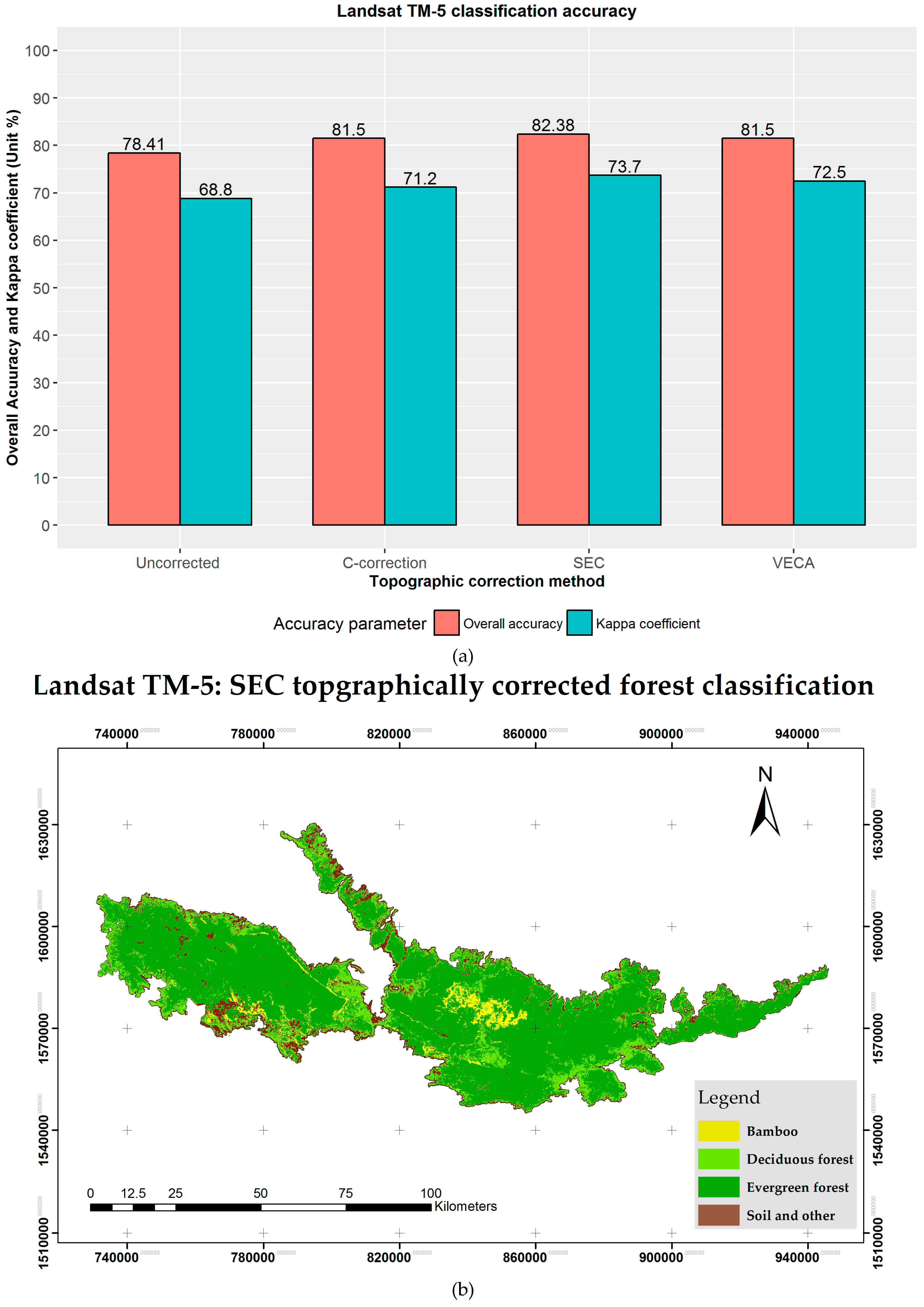
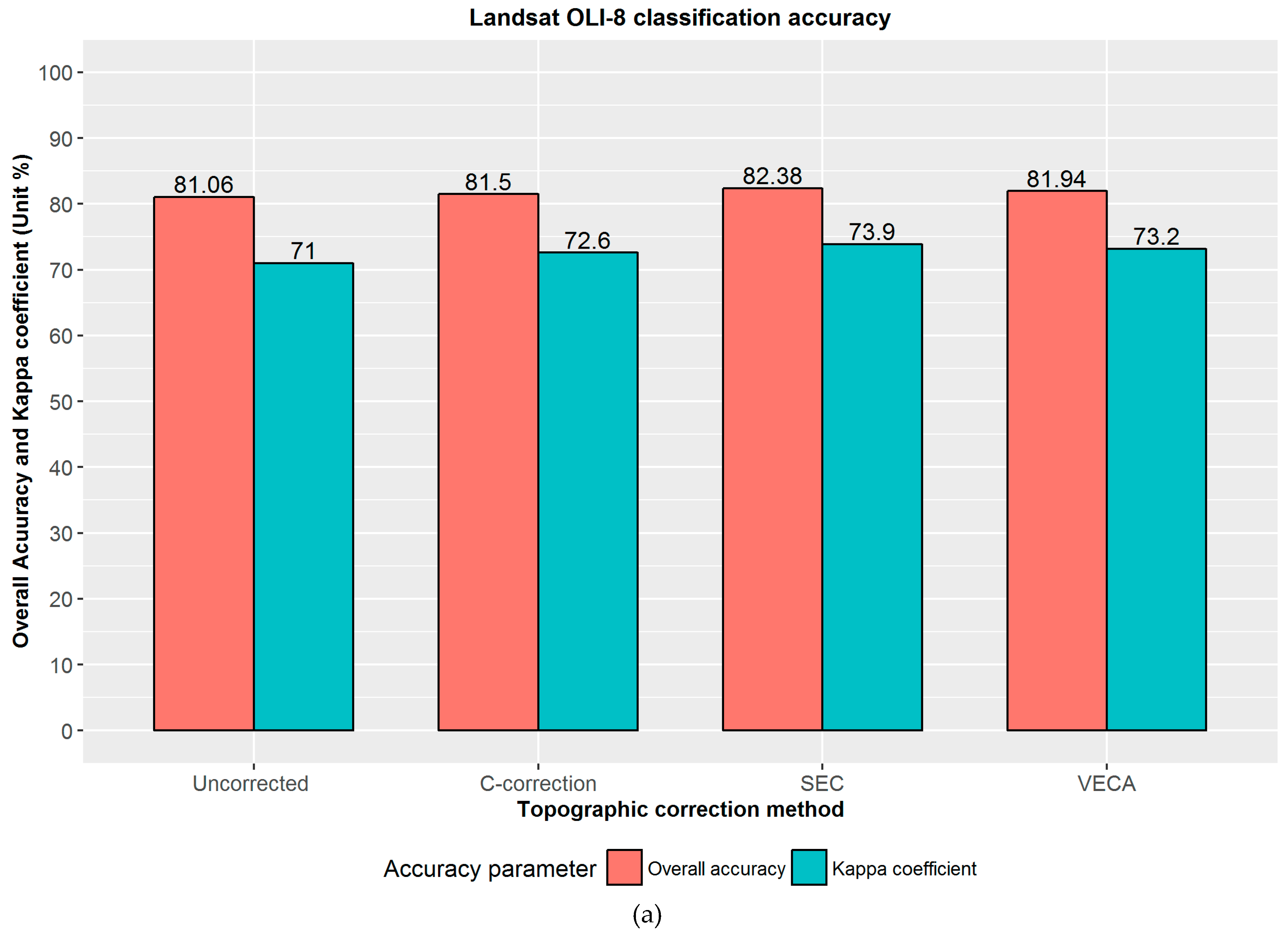
4.3. Evaluation of Topographically Corrected and Uncorrected Forest Classification Accuracies

An overview of RF classifications for various topographically corrected and uncorrected data from Landsat TM-5 and OLI-8 is presented in Figure 7 and Figure 8. In the above results, the improved cosine and Minnaert correction methods performed the worst with both DEMs, so we only used the results of SEC, VECA, and C-corrections for classification. Since visual interpretation and statistical evaluation suggest that the SRTM DEM is able to perform better than the ASTER GDEM, the results obtained from the C-correction, SEC and VECA topographic corrections using the SRTM DEM are used in the RF classification. The forest classifications presented here are based on the following scenarios: (a) Landsat TM-5 with the SRTM DEM; and (b) Landsat OLI-8 with the SRTM DEM. Figure 7 and Figure 8 shows the overall accuracy and Kappa coefficient of the RF machine learning classifier for the topographically uncorrected and C-correction, SEC, and VECA-corrected Landsat TM-5 and OLI-imagery.

Considering the overall accuracy, significant differences can be observed between the topographically corrected and uncorrected data from Landsat TM-5 and OLI-8. Forest classification based on the topographically uncorrected imagery shows an overall accuracy of 78.41% and a Kappa coefficient of 68.8%. After correction, the C-correction, SEC, and VECA-corrected data resulted an increase in overall accuracy, to 81.50 %, 82.38%, and 81.50%, respectively, as well as Kappa values of 71.2%, 73.7%, and 72.5%, respectively. Comparison of the uncorrected and corrected results reveals increases in overall accuracy of 3.09%, 3.97%, and 3.09%, and an increase in Kappa coefficient of 2.4%, 4.9% and 3.7%, respectively. Thus, for Landsat TM-5 imagery, the SEC-corrected imagery ranks highest for improved forest classification, with a 3.97% increase in overall accuracy and an increase in Kappa coefficient of 4.9% (Figure 7a). Figure 7b presents the forest classification of Landsat TM-5 obtained after SEC correction.

Similarly, Figure 8 shows the overall accuracy and Kappa coefficients of topographically corrected and uncorrected data from Landsat OLI-8. The overall accuracy of the uncorrected imagery was 81.06% with a Kappa coefficient of 71%. An increase in overall accuracy and Kappa coefficient similar to that described above can be seen in the Landsat OLI-8 imagery. Correction by the C-correction, SEC and VECA methods resulted in overall accuracies of 81.50%, 82.38%, and 81.94%, and Kappa values of 72.6%, 73.9%, and 73.2%, respectively. Thus, the topographic corrections result in increases in overall accuracy of 0.44%, 1.32%, and 0.88%, and an increases in Kappa values of 1.6 %, 2.9%, and 2.2%, respectively. Thus, for Landsat OLI-8 data, the SEC-corrected imagery ranks highest for improved forest classification, increasing the overall accuracy by 1.32% and the Kappa coefficient by 2.9% (Figure 8a). Figure 8b presents the forest classification of Landsat OLI-8 obtained after SEC.

In summary, the classification accuracies for topographically corrected imagery are higher than for uncorrected imagery. The results indicate that the Landsat TM-5 data are subject to a greater change in overall accuracy than the Landsat OLI-8 images. Thus, the results from this study suggest that the topographic effects within Landsat TM-5 and OLI-8 sensor imagery can be effectively reduced, with an increase in the overall accuracy of the RF classifier.

5. Discussion

5.1. Topographic Correction and DEMs

A major limitation of many topographic correction methods is the availability of a DEM of sufficient quality [10,21,26]. The recommended DEM resolution for effective removal of the topographic effect is one third the pixel size of Landsat images [26]. Owing to the limited availability of high-resolution DEMs and the poor accessibility to mountainous forest terrain, an evaluation of the full potential of freely available DEMs is essential. In this study, we have evaluated various topographic correction methods based on freely available multisource DEMs. We focused on Landsat TM-5 and OLI-8 imagery, which has a 30 m × 30 m resolution, as well as the freely available SRTM DEM and ASTER GDEM, both of which have a similar resolution. The recent availability of the SRTM DEM with 30 m × 30 m resolution allows for its direct comparison with the ASTER GDEM in the analysis of topographic correction methods. We showed that both DEMs are able to improve the topographic correction of satellite imagery, and it can therefore be concluded that both DEMs are suitable for removing the topographic effect from Landsat series imagery.

We found, however, that the performance of the topographic correction methods is greatly affected by the chosen DEM. In general, the SRTM DEM produced slightly superior results compared to the ASTER GDM for individual forest classes. The accuracies of corrections based on the ASTER GDEM may vary as a result of lower absolute vertical and horizontal errors and data noise in hilly areas [21,64,65]. On a larger scale, especially in forest regions with mountainous terrain, the quality of the ASTER GDEM-corrected imagery greatly varies from region to region, due to the presence of frequent cloud cover or low optical contrast in the source images [21,65]. However, it should be noted that the ability of radar (C-band) to penetrate clouds and dense vegetation gives the SRTM DEM an advantage over optical observations. The superior performance of the SRTM DEM in comparison with the ASTER GDEM is in line with previous studies [8,21,32,33,65,66,67].

In this study, the topographic correction performance varied, depending on the method and DEM used. Our results indicate that the C-correction, SEC, and VECA methods show the best performance with both DEMs. The improved cosine correction consistently overcorrects the imagery, as a result of the Lambertian reflectance assumptions [10,13,14,63]. Additionally, the algorithm for this method considers the mean illumination for forest strata instead of regression parameters calculated from the illumination and uncorrected reflectance [5]. The Minnaert correction method did not perform well either, especially in evergreen forests, which cover the majority of the study area. The Minnaert corrected image, which provides good visual appearance compared to the improved cosine correction, shows a decrease in the topographic effect. However, the Minnaert correction method with the slope included is unable to give good results, which was reported by Riaño et al. [10] and Hantson et al. [26]. The negative CV_Difference values within the heterogeneous deciduous forest shows the poorer performance in less sloping or flat terrain. Overall, we observed that the SEC method was able to correct the Landsat TM-5 and OLI-8 imagery better than the other correction methods. This is due consideration of a prior specification of forested pixels [48] and non-Lambertian assumption for forest class [5]. The C-correction and VECA also produces acceptable results, but the statistical evaluation suggests that SEC is superior. In addition, the comparison of shadow and non-shadow area proved the effectives of SEC correction method. The topographic correction results were seen to vary within heterogeneous forest types, primarily deciduous forests, occupying flatter terrain. In the deciduous forest, the C-correction and VECA perform slightly better than SEC. This implies that the regression parameters may be affected by the heterogeneity of forest types, and that further stratification and the creation of sub-forest strata could improve the correction of heterogeneous forest pixels [68].

5.2. Forest Classification Results and Accuracies

Our results showed that forest classification accuracy increased after topographic correction. For Landsat TM-5 and OLI-8 data, the increases in overall accuracy varied between 3% and 3.97%, and 0.44% and 1.34%, with increases in Kappa coefficient of 2.4% – 4.9% and 1.6% – 2.9%, respectively [32]. Further, in addition to the topographic correction methods, the performance of forest classification varies between forest cover types [69]. The classification of evergreen forests, bamboo, and non-forest areas was completed with the highest accuracy, but the greatest variation was found in the deciduous forest class. It is likely that the heterogeneous nature of this forest type makes it difficult to classify. As a result, the obtained accuracies were lower in this DF compared with the EF and BF classes. The highest misclassification rate was also found within the DF, as a result of its heterogeneous nature and highly fragmented distribution. The total area of deciduous forest accounts for only a small percentage of the total forest area in our study region, and are mostly located in less sloping terrain. The used Landsat imagery and field surveys from March, during which the deciduous forests drop their leaves, could be reason for the lower accuracy among deciduous forest types. An improved approach is therefore required to address this interclass variability in spectral response, since the phenological changes of a forest could affect the topographic correction as well as the accuracy of the classifiers. The spatial and temporal variations of specific forest types, such as deciduous forest, must be considered when applying topographic corrections.

Topographic corrections also lead to a small but significant improvement in the overall accuracy of the RF classifier. This approach is very useful for the detection and analysis of long term change using multiple sensors and multitemporal images from the Landsat series.

6. Conclusions

In this study, five topographic correction methods were evaluated by comparing their impact on the overall accuracy of forest classification algorithms. The topographic correction was performed using two DEMs: SRTM and ASTER GDEM DEMs. The results of the topographic correction indicate that a stratified approach using C-correction, SEC, and VECA correction methods was able to reduce the topographic effect within mountainous forest terrain, while preserving original reflectance values of an image. Among these, the SEC performs best with the SRTM 30 m × 30 m DEM, while the C-correction and VECA also produce acceptable corrections. It is expected that further sub-stratification of forest types and higher resolution DEMs could improve the results.

Compared with original Landsat series images (Landsat TM-5 and OLI-8), the topographically corrected images produce better forest classifications, which can be seen from the increase in overall accuracies and Kappa coefficient in the RF classifier. For Landsat TM-5, the SEC method improved classification accuracy by around 3.97%, while for Landsat OLI-8 the accuracy improvement was around 1.32%.

On the basis of this study, it is expected that advanced topographic corrections and machine learning RF classifier can be implemented within the sustainable mapping and monitoring of forest species in complex mountainous terrain. The main finding of the present study is that the newly available SRTM 30 m × 30 m DEM can be effectively used for the topographic correction of Landsat TM-5 and OLI-8 data for forest mapping studies in mountainous terrain.

Future research should focus on the application of topographic correction and classification to multitemporal imagery. The forest classification could also be further improved within heterogeneous forest types. The forest classification approach presented here can be used to improve accuracy across a variety of forestry applications such as forest type classification, forest species-based biomass or carbon estimation, and the monitoring of changes in forest species composition on larger scales. The application of newly available (ALOS) World 3D DEM is also recommended for future work [70].

References

1. Gu, D.; Gillespie, A. Topographic normalization of Landsat TM images of forest based on subpixel Sun-canopy-sensor geometry. Remote Sens. Environ. 1998, 64, 166–175. [Google Scholar] [CrossRef]
2. Roy, D.P.; Wulder, M.A.; Loveland, T.R.; Woodcock, C.E.; Allen, R.G.; Anderson, M.C.; Helder, D.; Irons, J.R.; Johnson, D.M.; Kennedy, R.; et al. Landsat-8: Science and product vision for terrestrial global change research. Remote Sens. Environ. 2014, 145, 154–172. [Google Scholar] [CrossRef]
3. Stibig, H.J.; Achard, F.; Carboni, S.; Raši, R.; Miettinen, J. Change in tropical forest cover of Southeast Asia from 1990 to 2010. Biogeosciences 2014, 11, 247–258. [Google Scholar] [CrossRef] [Green Version]
4. Li, M.; Im, J.; Beier, C. Machine learning approaches for forest classification and change analysis using multi-temporal Landsat TM images over Huntington Wildlife Forest. GISci. Remote Sens. 2013, 50, 361–384. [Google Scholar]
5. Szantoi, Z.; Simonetti, D. Fast and robust topographic correction method for medium resolution satellite imagery using a stratified approach. IEEE J. Sel. Top. Appl. Earth Obs. Remote Sens. 2013, 6, 1921–1933. [Google Scholar] [CrossRef]
6. Bruce, C.M.; Hilbert, D.W. Pre-processing Methodology for Application to Landsat TM/ETM+ Imagery of the Wettropics; Rainforest CRC: Cairns, Australia, 2004; p. 44. [Google Scholar]
7. Bodart, C.; Eva, H.; Beuchle, R.; Raši, R.; Simonetti, D.; Stibig, H.J.; Brink, A.; Lindquist, E.; Achard, F. Pre-processing of a sample of multi-scene and multi-date Landsat imagery used to monitor forest cover changes over the tropics. ISPRS J. Photogramm. Remote Sens. 2011, 66, 555–563. [Google Scholar] [CrossRef]
8. Adhikari, H.; Heiskanen, J.; Maeda, E.E.; Pellikka, P.K.E. Does topographic normalization of Landsat images improve fractional tree cover mapping in tropical mountains? ISPRS Int. Arch. Photogramm. Remote Sens. Spat. Inf. Sci. 2015, XL-7/W3, 261–267. [Google Scholar] [CrossRef]
9. Shepherd, J.D.; Dymond, J.R. Correcting satellite imagery for the variance of reflectance and illumination with topography. Int. J. Remote Sens. 2003, 24, 3503–3514. [Google Scholar] [CrossRef]
10. Riaño, D.; Chuvieco, E.; Salas, J.; Aguado, I. Assessment of different topographic corrections in Landsat-TM data for mapping vegetation types. IEEE Trans. Geosci. Remote Sens. 2003, 41, 1056–1061. [Google Scholar]
11. Dorren, L.K.; Maier, A.B.; Seijmonsbergen, A.C. Improved Landsat-based forest mapping in steep mountains terrain using object based classification. Forest Ecol. Manag. 2003, 183, 31–46. [Google Scholar] [CrossRef]
12. Hale, S.R.; Rock, B.N. Impact of topographic normalization on land-cover classification accuracy. Photogramm. Eng. Remote Sens. 2003, 69, 785–791. [Google Scholar] [CrossRef]
13. Huang, H.; Gongac, P.; Clintonc, N.; Huia, F. Reduction of atmospheric and topographic effect on Landsat TM data for forest classification. Int. J. Remote Sens. 2007, 29, 5623–5642. [Google Scholar] [CrossRef]
14. Tan, B.; Masek, J.G.; Wolfe, R.; Gao, F.; Huang, C.; Vermote, E.F.; Sexton, J.O.; Ederer, G. Improved forest change detection with terrain illumination corrected Landsat images. Remote Sens. Environ. 2013, 136, 469–483. [Google Scholar] [CrossRef]
15. Ke, L.; Tuong, T.; Van Hung, N. Correction of spectral radiance of optical satellite image for mountainous terrain for studying land surface cover changes. Geod. Cartogr. 2014, 63, 39–53. [Google Scholar] [CrossRef]
16. Cuo, L.; Vogler, J.B.; Fox, J.M. Topographic normalization for improving vegetation classification in a mountainous watershed in northern Thailand. Int. J. Remote Sens. 2010, 31, 3037–3050. [Google Scholar] [CrossRef]
17. Vanonckelen, S.; Lhermitte, S.; Rompaey, A.V. The effect of atmospheric and topographic corrections on pixel-based image composites: Improved forest cover detection in mountain environments. Int. J. Appl. Earth Obs. Geoinf. 2015, 35, 320–328. [Google Scholar] [CrossRef]
18. Tokola, T.; Sarkeala, J.; Van Der Linden, M. Use of topographic correction in Landsat TM-based forest interpretation in Nepal. Int. J. Remote Sens. 2001, 22, 551–563. [Google Scholar] [CrossRef]
19. Teillet, P.M.; Guindon, B.; Goodenough, D.G. On the slope-aspect correction of multispectral scanner data. Can. J. Remote Sens. 1982, 8, 84–106. [Google Scholar] [CrossRef]
20. Meyer, P.; Itten, K.I.; Kellenberger, T.; Sandmeier, S.; Sandmeier, R. Radiometric corrections of topographically induced effects on Landsat TM data in an alpine environment. ISPRS J. Photogram. Remote Sens. 1993, 48, 17–28. [Google Scholar] [CrossRef]
21. Wu, Q.; Jin, Y.; Fan, H. Evaluating and comparing performances of topographic correction methods based on multi-source DEMs and Landsat-8 OLI Data. Int. J. Remote Sens. 2016, 37, 4712–4730. [Google Scholar] [CrossRef]
22. Civco, D.L. Topographic normalization of landsat thematic mapper digital imagery. Photogram. Eng. Remote Sens. 1989, 55, 1303–1309. [Google Scholar]
23. Zakšek, K.; Čotar, K.; Veljanovski, T.; Pehani, P.; Oštir, K. Topographic correction module at storm (TC@Storm). ISPRS Int. Arch. Photogramm. Remote Sens. Spat. Inf. Sci. 2015, XL-7/W3, 721–728. [Google Scholar] [CrossRef]
24. Lu, D.; Ge, H.; He, S.; Xu, A.; Zhou, G.; Du, H. Pixel-based Minnaert correction method for reducing topographic effects on a Landsat 7 ETM+ image. Photogramm. Eng. Remote Sens. 2008, 74, 1343–1350. [Google Scholar]
25. Moreira, E.P.; Valeriano, M.M. Application and evaluation of topographic correction methods to improve land cover mapping using object-based classification. Int. J. Appl. Earth Obs. Geoinf. 2014, 32, 208–217. [Google Scholar] [CrossRef]
26. Hantson, S.; Chuvieco, E. Evaluation of different topographic correction methods for Landsat imagery. Int. J. Appl. Earth Obs. Geoinf. 2011, 13, 691–700. [Google Scholar] [CrossRef]
27. Kobayashi, S.; Sanga-Ngoie, K. The integrated radiometric correction of optical remote sensing imageries. Int. J. Remote Sens. 2008, 29, 5957–5985. [Google Scholar] [CrossRef]
28. Richter, R.; Kellenberger, T.; Kaufmann, H. Comparison of topographic correction methods. Remote Sens. 2009, 1, 184–196. [Google Scholar] [CrossRef] [Green Version]
29. Sola, I.; González-Audícana, M.; Álvarez-Mozos, J. The added value of stratified topographic correction of multispectral images. Remote Sens. 2016, 8, 131. [Google Scholar] [CrossRef]
30. Gao, Y.; Zhang, W. Variable empirical coefficient algorithm for removal of topographic effects on remotely sensed data from rugged terrain. Int. Geosci. Remote Sens. Symp. 2007, 1, 4733–4736. [Google Scholar]
31. Gao, Y.; Zhang, W. A simple empirical topographic correction method for ETM+ imagery. Int. J. Remote Sens. 2009, 30, 2259–2275. [Google Scholar] [CrossRef]
32. Vanonckelen, S.; Lhermitte, S.; Van Rompaey, A. The effect of atmospheric and topographic correction methods on land cover classification accuracy. Int. J. Appl. Earth Obs. Geoinf. 2013, 24, 9–21. [Google Scholar] [CrossRef]
33. Vanonckelen, S.; Lhermitte, S. Performance of atmospheric and topographic correction methods on Landsat imagery in mountain areas. Int. J. Remote Sens. 2014, 35, 4952–4972. [Google Scholar] [CrossRef]
34. Blesius, L.; Weirich, F. The use of the Minnaert correction for land-cover classification in mountainous terrain. Int. J. Remote Sens. 2005, 26, 3831–3851. [Google Scholar] [CrossRef]
35. Gitas, I.Z.; Devereux, B.J. The role of topographic correction in mapping recently burned Mediterranean forest areas from Landsat TM images. Int. J. Remote Sens. 2006, 27, 41–54. [Google Scholar] [CrossRef]
36. Soenen, S.A.; Peddle, D.R.; Coburn, C.A.; Hall, R.J.; Hall, F.G. Improved topographic correction of forest image data using a 3-D canopy reflectance model in multiple forward mode. Int. J. Remote Sens. 2008, 29, 1007–1027. [Google Scholar] [CrossRef]
37. She, X.; Zhang, L.; Cen, Y.; Wu, T.; Huang, C.; Baig, M.H.A. Comparison of the continuity of vegetation indices derived from Landsat 8 OLI and Landsat 7 ETM+ data among different vegetation types. Remote Sens. 2015, 7, 13485–13506. [Google Scholar] [CrossRef]
38. Thai National Parks. Available online: https://www.thainationalparks.com/khao-yai-national-park (accessed on 19 October 2015).
39. Khao Yai National Park. Available online: https://en.wikipedia.org/wiki/Khao_Yai_National_Park (accessed on 19 October 2015).
40. The Land Processes Distributed Active Archive Center. Available online: https://lpdaac.usgs.gov/data_access/glovis (accessed on 10 February 2016).
41. The Shuttle Radar Topographic Mission (SRTM). Available online: https://lta.cr.usgs.gov/SRTM (accessed on 30 July 2016).
42. Advanced Spaceborne Thermal Emission and Reflection Radiometer (ASTER) Global Digital Elevation Model (GDEM). Available online: http://earthexplorer.usgs.gov/ (accessed on 10 February 2016).
43. McDonald, E.R.; Wu, X.; Caccetta, P.A.; Campbell, N.A. Illumination correction of Landsat TM data in South East NSW. In Proceedings of the Tenth Australasian Remote Sensing Conference, Adelaide, Australia, 21–25 August 2000.
44. Machala, M. Forest mapping through object-based image analysis of multispectral and LiDAR aerial data. Eur. J. Remote Sens. 2014, 47, 117–131. [Google Scholar] [CrossRef]
45. Goslee, S.C. Analyzing remote sensing data in R: The Landsat Package. J. Stat. Softw. 2011, 43, 1–25. [Google Scholar] [CrossRef]
46. Smith, J.A.; Lin, T.L.; Ranson, K.J. The Lambertian assumption and Landsat data. Photogram. Eng. Remote Sens. 1980, 46, 1183–1189. [Google Scholar]
47. Ediriweera, S.; Pathirana, S.; Danaher, T.; Nichols, D.; Moffiet, T. Evaluation of different topographic corrections for Landsat TM data by Prediction of Foliage Projective Cover (FPC) in topographically complex landscapes. Remote Sens. 2013, 5, 6767–6789. [Google Scholar] [CrossRef]
48. Wulder, M.A.; Franklin, S.E. Remote Sensing of Forest Environments: Concepts and Case Studies; Springer: New York, NY, USA, 2003; p. 200. [Google Scholar]
49. Karathanassi, V.; Andronis, V.; Rokos, D. Evaluation of the topographic normalization methods for a Mediterranean forest area. Int. Arch. Photogramm. Remote Sens. 2000, 33, 654–661. [Google Scholar]
50. Olofsson, P.; Foody, G.M.; Herold, M.; Stehman, S.V.; Woodcock, C.E.; Wulder, M.A. Good practices for estimating area and assessing accuracy of land change. Remote Sens. Environ. 2014, 148, 42–57. [Google Scholar] [CrossRef]
51. FAO. Map Accuracy Assessment and Area Estimation Map Accuracy Assessment and Area Estimation: A Practical Guide; FAO: Rome, Italy, 2016; p. 12. [Google Scholar]
52. Liang, L.; Chen, Y.; Hawbaker, T.; Zhu, Z.; Gong, P. Mapping mountain Pine beetle mortality through growth trend analysis of time-series Landsat data. Remote Sens. 2014, 6, 5696–5716. [Google Scholar] [CrossRef]
53. Breiman, L. Random Forests. Mach. Learn. 2001, 45, 5–32. [Google Scholar] [CrossRef]
54. Liaw, A.; Wiener, M. Classification and Regression by randomForest. R News 2002, 2, 18–22. [Google Scholar]
55. Immitzer, M.; Vuolo, F.; Atzberger, C. First experience with Sentinel-2 data for crop and tree species classifications in central Europe. Remote Sens. 2016, 8, 166. [Google Scholar] [CrossRef]
56. Liu, J.; Heiskanen, J.; Aynekulu, E.; Maeda, E.E.; Pellikka, P.K.E. Land cover characterization in west Sudanian savannas using seasonal features from annual Landsat time series. Remote Sens. 2016, 8, 365. [Google Scholar] [CrossRef]
57. Lowe, B.; Kulkarni, A. Multispectral image analysis using random forest. Int. J. Soft Comput. 2015, 6, 1–14. [Google Scholar] [CrossRef]
58. Shen, W.; Li, M.; Huang, C.; Wei, A. Quantifying live aboveground biomass and forest disturbance of mountainous natural and plantation forests in Northern Guangdong, China, based on multi-temporal Landsat, PALSAR and field plot data. Remote Sens. 2016, 8, 595. [Google Scholar] [CrossRef]
59. R Core Team. R: A Language and Environment for Statistical Computing; R Foundation for Statistical Computing: Vienna, Austria, 2016. [Google Scholar]
60. Benjamin Leutner and Ned Horning. RStoolbox: Tools for Remote Sensing Data Analysis. R Package Version 0.1.4. 2016. Available online: https://CRAN.R-project.org/package=RStoolbox (accessed on 19 October 2016).
61. QGIS Development Team. QGIS Geographic Information System. Open Source Geospatial Foundation Project. 2016. Available online: http://www.qgis.org/ (accessed on 19 October 2016).
62. Foody, G.; Hill, R. Classification of tropical forest classes from Landsat TM data. Int. J. Remote Sens. 1996, 17, 2353–2367. [Google Scholar] [CrossRef]
63. Gao, M.L.; Zhao, W.J.; Gong, Z.N.; Gong, H.L.; Chen, Z.; Tang, X.M. Topographic correction of ZY-3 satellite images and its effects on estimation of shrub leaf biomass in mountainous areas. Remote Sens. 2014, 6, 2745–2764. [Google Scholar] [CrossRef]
64. Wang, L.; Chen, J.; Zhang, H.; Chen, L. Difference analysis of SRTM C-Band DEM and ASTER GDEM for global land cover mapping. In Proceedings of the 2011 International Symposium on Image and Data Fusion (ISIDF), Tengchong, Yunnan, China, 9–11 August 2011.
65. Hirt, C.; Filmer, M.S.; Featherstone, W.E. Comparison and validation of the recent freely available ASTER-GDEM ver1, SRTM ver4.1 and GEODATA DEM-9S ver3 digital elevation models over Australia. Aust. J. Earth Sci. 2010, 57, 337–347. [Google Scholar] [CrossRef]
66. Balthazar, V.; Vanacker, V.; Lambin, E.F. Evaluation and parameterization of ATCOR3 topographic correction method for forest cover mapping in mountain areas. Int. J. Appl. Earth Obs. Geoinf. 2012, 18, 436–450. [Google Scholar] [CrossRef]
67. Frey, H.; Paul, F. On the suitability of the SRTM DEM and ASTER GDEM for the compilation of: Topographic parameters in glacier inventories. Int. J. Appl. Earth Obs. Geoinf. 2012, 18, 480–490. [Google Scholar] [CrossRef]
68. Sandmeier, S.; Itten, K.I. A Physically-based model to correct atmospheric and illumination effects in optical satellite data of rugged terrain. IEEE Trans. Geosci. Remote Sens. 1997, 35, 708–717. [Google Scholar] [CrossRef]
69. Kachmar, M.; Sanchez-Azofeifa, G.A.; Rivard, B.; Kakubari, Y. Improved forest cover classification in an industrialized mountain area in Japan. Mt. Res. Dev. 2005, 25, 349–356. [Google Scholar] [CrossRef]
70. Santillan, J.R.; Makinano-Santillan, M. Vertical accuracy assessment of 30-M resolution ALOS, ASTER, and SRTM Global DEMS over northeastern Mindanao, Philippines. ISPRS Int. Arch. Photogramm. Remote Sens. Spat. Inf. Sci. 2016, XLI-B4, 149–156. [Google Scholar] [CrossRef]
Figure 1. Effect of irregular mountain terrain on the reflectance of Landsat Thematic Mapper (TM)-5 and Operational Land Imager (OLI)-8 images (Path/row: 129/050, TM-5: 9 February 1999, OLI-8: 2 February 2015): (a) Hillshade: the hypothetical illumination of a surface calculated using the Shuttle Radar Topography Mission (SRTM) Digital Elevation Model (DEM), the solar zenith, and azimuth angles; (b) Hillshade: the hypothetical illumination of a surface calculated using Advanced Spaceborne Thermal Emission and Reflection Radiometer (ASTER) Global Digital Elevation Model (GDEM), the solar zenith, and azimuth angles; (c) false color composite Landsat TM-5 bands 5, 4, and 3; (d) Landsat TM-5 near infrared (NIR) band 4; (e) false color composite Landsat OLI-8 bands 6, 5, and 4; and (f) Landsat OLI-8 NIR band 5.
Sustainability 09 00258 g001
Figure 2. Study area: The Dong Phayayen-Khao Yai Forest Complex.
Sustainability 09 00258 g002
Figure 3. Flow diagram showing the detailed research methodology of topographic correction, Random Forest (RF) supervised classification, and validation.
Sustainability 09 00258 g003
Figure 4. Locations of training and validation sample points in the study area. A total of 767 randomly sampled points were created, of which 252 were randomly set aside as validation points. Green points show the locations of training data, red points show the locations of validation sample points.
Sustainability 09 00258 g004
Figure 5. Comparison of false color composites of Landsat TM-5 (band 5-4-3) image with SRTM DEM: (a) SRTM DEM; (b) Illumination based on SRTM; (c) Original image; (d) Improved cosine correction; (e) C-correction; (f) Minnaert correction; (g) Statistical-empirical correction (SEC); and (h) Variable Empirical Coefficient Algorithm (VECA); and comparison of false color composite of Landsat TM-5 (band 5-4-3) image with ASTER GDEM: (i) ASTER GDEM; (j) Illumination based on ASTER GDEM; (k) Original image; (l) Improved cosine correction; (m) C-correction; (n) Minnaert correction; (o) Statistical-empirical correction; and (p) VECA.
Sustainability 09 00258 g005
Figure 6. Comparison of false color composite of Landsat OLI-8 (band 6-5-4) image with SRTM DEM: (a) SRTM DEM; (b) Illumination based on SRTM; (c) Original image; (d) Improved cosine correction; (e) C-correction; (f) Minnaert correction; (g) Statistical-empirical correction; and (h) Variable Empirical Coefficient Algorithm (VECA); and comparison of false color composite of Landsat OLI-8 (band 6-5-4) image with ASTER GDEM: (i) ASTER GDEM; (j) Illumination based on ASTER GDEM; (k) Original image; (l) Improved cosine correction; (m) C-correction; (n) Minnaert correction; (o) Statistical-empirical correction; and (p) VECA.
Sustainability 09 00258 g006
Figure 7. (a) Overall accuracy and Kappa coefficients of forest classifications obtained from the RF classifier for Landsat TM-5 data; (b) Forest classification map obtained after SEC topographic correction.
Sustainability 09 00258 g007
Figure 8. (a) Overall accuracy and Kappa coefficients of forest classifications obtained from the RF classifier for Landsat OLI-8 data; (b) Forest classification map obtained after SEC topographic correction.
Sustainability 09 00258 g008aSustainability 09 00258 g008b