The Emergency Vehicle Routing Problem with Uncertain Demand under Sustainability Environments

Abstract

The reasonable utilization of limited resources is critical to realize the sustainable developments. In the initial 72-h crucial rescue period after the disaster, emergency supplies have always been insufficient and the demands in the affected area have always been uncertain. In order to improve timeliness, utilization and sustainability of emergency service, the allocation of the emergency supplies and the emergency vehicle routes should be determined simultaneously. Assuming the uncertain demands follow normal distribution, an optimization model for the emergency vehicle routing, by considering the insufficient supplies and the uncertain demands, is developed. The objective function is applied to minimize the total costs, including the penalty costs induced by more or less supplies than the actual demands at all demand points, as well as the constraints of the time windows and vehicle load capacity taken into account. In more details, a solution method for the model, based on the genetic algorithm, is proposed, which solves the problem in two stages. A numerical example is presented to demonstrate the efficiency and validity of the proposed model and algorithm.

1. Introduction

In recent years, around the world, natural disasters, such as earthquake, hurricane, volcanic eruption and flood, are occurring increasingly frequently. More than 500 disasters are estimated to strike our planet every year, killing around 75,000 people and impacting more than 200 million others [1]. For example, the Wenchuan Earthquake in China left more than 110,000 casualties in 2008, including 69,197 confirmed dead and 374,176 injured, with 18,222 listed as missing. The Haiti earthquake in 2010 caused 230,000 death and more than 300,000 injuries.

The enormous scale of these disasters has called attention to the need for effective and sustainable management of the relief activities after disasters. To mitigate damage and loss in disasters, issues in pre-disaster, during-disaster and post-disaster have been widely studied in the past few years. For relief activities in post-disaster, to transport sufficient emergency supplies to affected areas in order to support basic needs for those trapped in disaster-affected areas is a critical challenge [2]. Emergency supplies that are essential for human survivals include water, food and medicines. After the disaster, the supplies must be delivered to the demand points immediately, especially in the initial rescue period, which is the optimal rescue period for the people in the affected areas. Unfortunately, emergency resources are always restricted in this period. Therefore, it is necessary to enhance the sustainability of the emergency service to make full use of the resources. Thus, the effectiveness and timeliness of the delivery are significant to the humanitarian response and the sustainability of the rescue operation, which provide the motivation for this work.

Disasters always result in massive demands that often outstrip available resources. The process of planning, managing, and controlling the flow of those resources to provide relief to affected people is called emergency logistics. Different from general business logistics, emergency logistics is unique in some aspects that may increase the relative complexity in solving the induced problems. First, the demand-related information, e.g., the density of demand in the affected points, is quite limited in the initial rescue period, and is intuitively unpredictable using historical data. The lack of relevant information will lead to difficulties to determine the actual demands of the areas. Second, relative to general business logistics, the emergency resources may be insufficient to decision makers in the initial rescue period, since the disaster is unpredictable. This fact adds more challenging issues to the management of emergency logistics. Consequently, in order to improve the utilization-efficiency and delivery-timeliness of the limited resources in the initial rescue period, the distribution of emergency supplies and emergency vehicles routing has to be determined synchronously under the uncertainty conditions. Emergency logistics has emerged as a worldwide noticeable theme as disasters, either artificial or natural, may occur anytime around the world with enormous consequences [3].

The crucial rescue period refers to the initial 72 h following the onset of a disaster, which is regarded as the most critical period to search and rescue the trapped survivals [4]. In the crucial rescue period, the available emergency resources, including vehicles and supplies, are always limited. How to establish an effective emergency logistics system after emergency events, and launch the emergency plan to distribute the limited resources to the affect areas with a good planning and scheduling transportation, has been a research hotspot in recent decades.

The operations of emergency logistics are based on the timely delivery services and supplies allocation. In most cases, the vehicles are the most frequently used tools to implement the delivery work. Therefore, how to assign the work to existed vehicles and how to select the vehicle routes, namely, the emergency vehicle routing problem (VRP), are the key to the entire emergency logistics operations. Thus far, there have been many relevant studies on the VRP. Lei et al. [5], Zhu et al. [6], Errico et al. [7] and Zhang et al. [8] considered the VRP with time windows and stochastic service times. Yin and Chuang [9] first addressed a previously studied problem, then proposed a new problem version for planning the least cost routing, in which the deployed green vehicles transport the final products from suppliers to customers through a cross-dock subject to a CO₂ intensity constraint, and developed an adaptive memory artificial bee colony algorithm to tackle both problems. In their recent study [10], they proposed a bi-objective mathematical formulation for the cross-docking with interrelated operations (vehicle routing and vehicle scheduling), and developed a cooperative coevolution approach consisting of hyper-heuristics and hybrid-heuristics for achieving continuous improvement in alternating objectives. Marinakis et al. [11] introduced a new hybrid algorithmic approach based on particle swarm optimization for the vehicle routing problem with stochastic demands that are known only when the vehicle arrives to the customers. This algorithm is a combination of the particle swarm optimization algorithm with the 2-opt and 3-opt local search algorithms and with the path relinking strategy. Euchi et al. [12] described hybrid iterated density estimation evolutionary algorithm with 2-opt local search to determine the specific assignment of each tour to a private vehicle (internal fleet) or an outside carrier (external fleet).

Furthermore, Parragh et al. [13,14] wrote a survey about pickup and delivery problems, which are distinguished by two problem classes: the first class deals with the transportation of goods from the depot to line haul customers and from backhaul customers to the depot, and the second class refers to all those problems where goods are transported between pickup and delivery locations. Berghida and Boukra [15] dealt with the vehicle routing problem with simultaneous pickup and delivery by a new technique based on a cooperative approach reaping the benefits of three metaheuristics. Maquera et al. [16] presented an application of scatter search to the problem of routing vehicles that are required to deliver and pickup goods, which generates all pairs of solutions that contain at least one new element.

However, as we mentioned above, the emergency VRP is different from general VRP in demand-related information and supply of emergency resources, which bring more complexity to the problem. Wohlgemuth et al. [17] considered the dynamic vehicle routing problem with anticipation in disaster relief. Pillac et al. [18] classified routing problems from the perspective of information quality and evolution, introduced the notion of degree of dynamism, and presented a comprehensive review of applications and solution methods for dynamic vehicle routing problems. While Cao et al. [19] proposed four robust strategies to cope with the uncertain demand of an open VRP, Moghaddama et al. [20] investigated a variant of an uncertain VRP that the customer’s demands are supposed to be uncertain with unknown distributions. In addition, an advanced particle swarm optimization (PSO) algorithm was proposed to solve such VRP with a novel decoding scheme.

Despite the critical importance of emergency logistics distribution, only a limited amount of related studies have been carried out. Sheu [21] presented relief-demand management model for emergency logistics operations under imperfect information conditions. Lin et al. [2] proposed a logistics model for delivery of prioritized items in disaster relief operations. Chang et al. [22] gave a novel algorithm capability of regulating the distribution of available resources and automatically generating a variety of feasible emergency logistics schedules for decision-makers. In addition, Wang et al. [23] constructed a nonlinear integer open location-routing model for relief distribution problem in emergency logistics, considering travel time, the total cost, and reliability with split delivery.

The VRP is a problem with NP-difficulty, and this nature makes the exact algorithms only for small problems. For larger instances, heuristics is a natural choice. Therefore, much attention has been focused on designing heuristics algorithms with good performance. Following the first heuristics algorithm presented by Hochbaum and Shmoys [24], there has been a long list of work on designing heuristics algorithms for this problem over the years. Several meta-heuristic approaches were reported, including Genetic Algorithm (GA) [25,26,27], Tabu Search (TS) [28,29,30], Particle Swarm Optimization (PSO) [11,20,31], hybrid algorithm [32,33,34,35], etc., which were used to solve VRP and its variant problems. With reference to Genetic Algorithm, Ombuki et al. [25] proposed an application of genetic algorithms approach for multi-depot vehicle routing problem(MDVRP) using the Pareto ranking technique. An advantage of this approach is that it is unnecessary to derive weights for a weighted sum scoring formula. Furthermore, Ursani et al. [26] introduced the Localized Optimization Framework (LOF) which is an iterative procedure between two phases, Optimization and De-optimization. They have also chosen a genetic algorithm as an optimization methodology. It was demonstrated that the LGA is, on average, able to produce better solutions than most of the other heuristics on small scale problems of VRPTW. Moreover, the LGA has attained several new best solutions on popular datasets.

In the existing research results, the goal is all about minimizing the number of vehicles, vehicle travel distance and some other economic factors. However, this approach does not work with a full consideration of the distinguishing features in the crucial rescue period of relief operation, which may be in short supply and with uncertain demands. The main research of this paper is to fully consider the supply/demand features in crucial rescue period, and the optimization model for the emergency vehicle routing problem is developed. As for the solution methods, the particularity and practicality of the emergency vehicle routing problem are taken into consideration. This fact divides the problem into two stages, in which the first stage is to determine the serviced demand point set of each center, and the second stage is to optimize the used vehicle number, the actual supplies and vehicle routes at each center.

This paper is organized as follows. The mathematical model for the problem and the solution methods for the model are proposed in Section 2. In Section 3, numerical examples are presented to demonstrate the benefit of our new logistics model. Finally, the conclusions and suggestions for future work are given in Section 4.

2. Mathematical model and Methods

2.1. Model Foundation and Notations

A well-known challenge to efficiently execute disaster relief operations is to obtain sufficient and accurate demand information from the disaster-affected area. Due to the chaotic situation in the critical period, the information is always incomplete and inaccurate. Therefore, it becomes very difficult to correctly estimate useful information to deliver the emergency supplies. As a result, the precise emergency demands are uncertain due to the unpredictability of the actual demands at the demand points. In this paper, we assume that the demand at each point is uncertain with a known probability distribution. For example, we could define the actual demand at demand point $k$ as $d_k$, which is a random variable with probability density function given by $f_k\left(x\right)$. The probability distribution of demand is assumed to be available, which could derive from population data and/or information gathered during the disaster prevention phase [36].

Similar to the general vehicle routing problem, we also assume that all the emergency vehicles are the same type. In the initial period of rescue, a variety of rescue facilities and resources are very limited, so it is necessary to take as many emergency demand points as possible into account in this period, provide some necessities for them to ensure that they could wait for the subsequent rescue. In this case, we assume that the delivery for each demand point can be only served by one vehicle one time, which should return back to the starting point (service central) after finishing the current rescue mission.

For the sake of simplicity, the service time of vehicles on the demand point is included in travel time. The affected points considered in this paper are connected by existing roads, which can be serviced by vehicles. Other isolated points could be serviced by other methods, such as helicopters.

In formulating the mathematical model, the following notations in

Table 1. Symbols and Notations.

Symbol	Description
$\mathit{D}\mathit{N}$	Set of emergency demand point (affected point).
$\mathit{S}\mathit{N}$	Set of emergency supply point (service central).
$\mathit{N}$	$N=DN{\displaystyle \cup }SN$.
$\mathit{V}$	Set of vehicle, $v\in V$.
${\mathit{d}}_{\mathit{k}}$	Actual (uncertain) demand for emergency supplies at demand point $k\in DN$, which is a random variable.
${\mathit{z}}_{\mathit{k}}$	Assigned amount of emergency supplies at demand point $k$.
${\mathit{f}}_{\mathit{k}}\left(\mathit{x}\right)$	Probability density function of demand at demand point $k$.
${\mathit{t}}_{\mathit{k}}^{\mathit{v}}$	The time that the vehicle $v$ arrives at the demand point $k$.
${\mathit{T}}_{\mathit{k}}$	The latest time that the affected point $k$ can receive the emergency supplies, $k\in DN$.
${\mathit{t}}_{\mathit{i}\mathit{j}}$	Travel time from point $i$ to point $j$.
${\mathit{l}}_{\mathit{i}\mathit{j}}$	Distance between point $i$ and point $j$.
${\mathit{c}}_{\mathit{i}\mathit{j}}$	Transportation cost per kilometer from point $i$ to point $j$.
${\mathit{\omega }}_{\mathit{v}}$	Fixed costs of vehicle $v$ for delivery one time.
${\mathit{\tau }}_{\mathit{k}}^{-}$	Penalty cost per unit supplies for shortage in any demand point $k$.
${\mathit{\tau }}_{\mathit{k}}^{+}$	Penalty cost per unit supplies for surplus in any demand point $k$.
${\mathit{\theta }}_{\mathit{i}}$	Maximum number of available vehicles at service center $i,i\in SN$.
$\mathit{Q}$	Maximum load capacity of a vehicle.
$\mathit{M}$	A large enough positive number.

are used in this paper.

The decision variable is defined as follows:

$$X_{ij}^v=\{\begin{array}{c}1\mathrm{if}\mathrm{node}j\mathrm{is}\mathrm{the}\mathrm{next}\mathrm{node}\mathrm{to}\mathrm{node}i\mathrm{on}\mathrm{the}\mathrm{route}\mathrm{of}\mathrm{vehicle}v;\\ 0\mathrm{otherwise};\end{array}i,j\in N,v\in V$$

2.2. Mathematical Model

In this section, the mathematical model for the emergency vehicle routing problem and insufficient supplies is constructed, based on the above assumptions and notations.

As mentioned previously, emergency supplies are often insufficient in the 72-h crucial rescue period after disasters. Due to the significance of the availability of emergency resource at the demand points, a relatively large penalty ${\tau }_k^{-}$ is associated with the shortage of a unit of supply at demand point $k$, and this penalty corresponds to the social cost of a death or a severe injury of a patient because of a supply shortage. On the contrary, since the total amount of emergency supplies are limited, some demand points may suffer from a shortage, while others are assigned even more supplies. Henceforth, the penalty ${\tau }_k^{+}$ is also assigned to a possible supply surplus, in terms of units. In other words, the amount of emergency supplies distributed to each demand point should be consistent with that of actual demands as soon as possible, and both the excessive and insufficient distribution could effect on rescue. Similar examples of penalty costs, due to excessive supplies, as well as shortages, can be found in the literature [37,38]. These penalties should be considered in the objective function of the model to measure the utilization efficiency of the limited supplies.

Specifically, for any point $k\in DN$, when the delivered emergency supply is not equal with its actual demand, the amount of shortage $∆d_k^{-}$ and surplus $∆d_k^{+}$ can be calculated, respectively, as follows:

$$∆d_k^{-}=max\left\{0,d_k-z_k\right\}$$

(1)

$$∆d_k^{+}=max\left\{0,z_k-d_k\right\}$$

(2)

According to the definition of notations, the probability of the supply shortage ($P_k^{-}\left(z_k\right)$) and supply surplus ($P_k^{+}\left(z_k\right)$) at demand point $k$ can be expressed, respectively, as:

$$P_k^{-}\left(z_k\right)=P_k\left(d_k\le z_k\right)={{\displaystyle \int }}_0^{z_k}{f}_k\left(x\right)d_x,\forall k\in DN$$

(3)

$$P_k^{+}\left(z_k\right)=P_k\left(d_k\ge z_k\right)={{\displaystyle \int }}_{z_k}^{+\infty }{f}_k\left(x\right)d_x,\forall k\in DN$$

(4)

Hence, the expected amount of the shortage ($E\left(∆d_k^{-}\right)$) or surplus ($E\left(∆d_k^{+}\right)$) at demand point $k$ can be calculated by:

$$E\left(∆d_k^{+}\right)={{\displaystyle \int }}_0^{z_k}\left(z_k-x\right)f_k\left(x\right)d_x$$

(5)

$$E\left(∆d_k^{-}\right)={{\displaystyle \int }}_{z_k}^{+\infty }\left(x-z_k\right)f_k\left(x\right)d_x$$

(6)

Based on the above quantities, the expected penalties incurred by the distribution decision due to the shortage and surplus of the relief supplies at each demand point can be easily calculated.

In addition, the available rescue vehicles are always limited in the 72-h crucial rescue period, so it is better to finish the rescue work with fewer vehicles. For this purpose, the operating costs of vehicles should be measured in the objective function of the model, which could be described as:

$${{\displaystyle \sum }}_{v\in V}{{\displaystyle \sum }}_{i\in SN}{{\displaystyle \sum }}_{j\in DN}{\omega }_v{X}_{ij}^v$$

(7)

According to the above analysis, the optimization model of the emergency vehicle route considering insufficient supplies can be established as follows:

$$\begin{array}{c}\min \phi ={\displaystyle {\displaystyle \sum }_{k\in DN}}\left({\tau }_k^{-}{{\displaystyle \int }}_{z_k}^{+\infty }\left(x-z_k\right)f_k\left(x\right)d_x+{\tau }_k^{+}{{\displaystyle \int }}_0^{z_k}\left(z_k-x\right)f_k\left(x\right)d_x\right)\\ +{{\displaystyle \sum }}_{v\in V}{{\displaystyle \sum }}_{i\in N}{{\displaystyle \sum }}_{j\in N}{c}_{ij}{l}_{ij}{X}_{ij}^v+{{\displaystyle \sum }}_{v\in V}{{\displaystyle \sum }}_{i\in SN}{{\displaystyle \sum }}_{j\in DN}{\omega }_v{X}_{ij}^v\end{array}$$

(8)

$$s.t.{{\displaystyle \sum }}_{i\in N}{{\displaystyle \sum }}_{k\in DN}{X}_{ik}^v{z}_k\le Q,\forall v\in V$$

(9)

$${{\displaystyle \sum }}_{j\in DN}{X}_{ij}^v\le {\vartheta }_i,\forall i\in \mathrm{S}N$$

(10)

$$t_i^v+t_{ij}-t_j^v\le (1-X_{ij}^v)\mathrm{M},\forall i,j\in DN,\forall v\in V$$

(11)

$$t_i^v+t_{ij}-t_j^v\le (1-X_{ij}^v)\mathrm{M},\forall i,j\in DN,\forall v\in V$$

(12)

$${{\displaystyle \sum }}_{j\in SN}{X}_{ji}^v={{\displaystyle \sum }}_{j\in SN}{X}_{ij}^v=0,\forall i\in SN,\forall v\in V$$

(13)

$${{\displaystyle \sum }}_{j\in DN}{X}_{ij}^v={{\displaystyle \sum }}_{j\in DN}{X}_{ji}^v\le 1,\forall i\in SN,\forall v\in V$$

(14)

$${{\displaystyle \sum }}_{v\in V}{{\displaystyle \sum }}_{j\in DN}{X}_{ij}^v=1,\forall i\in N$$

(15)

$$X_{ji}^v\in \left\{0,1\right\},\forall i,j\in N,\forall v\in V$$

(16)

In this model, the objective function (Equation (8)) is to minimize the total expected cost, in which ${{\displaystyle \sum }}_{k\in DN}\left({\tau }_k^{-}{{\displaystyle \int }}_{z_k}^{+\infty }\left(t-z_k\right)f_k\left(t\right)d_t\right)$ is the total expected shortage penalty incurred by the insufficient supply at demand points, ${{\displaystyle \sum }}_{k\in DN}\left({\tau }_k^{+}{{\displaystyle \int }}_0^{z_k}\left(z_k-t\right)f_k\left(t\right)d_t\right)$ is the total expected surplus penalty incurred by the excessive supply at demand points, ${{\displaystyle \sum }}_{i\in N}{{\displaystyle \sum }}_{j\in N}{{\displaystyle \sum }}_{v\in V}{c}_{ij}{l}_{ij}{X}_{ij}^v$ is the total transportation costs, and ${{\displaystyle \sum }}_{v\in V}{{\displaystyle \sum }}_{i\in SN}{{\displaystyle \sum }}_{j\in DN}{\omega }_v{X}_{ij}^v$ is the total operating costs of vehicles.

In addition to the objective, Constraint (9) represents the load capacity constraint of a vehicle. Constraint (10) ensures that the vehicles which depart from a service central are no more than the maximum available vehicles in the center. Constraint (11) determines the time that the vehicle arrives at the demand points. Constraint (12) gives the time that the vehicle arrives at the demand point, in which the service time window must be satisfied. Constraint (13) ensures the emergency vehicles cannot travel between the service centers. Constraint (14) indicates that all the vehicles should start the delivery work from a service center and return to the same center after these missions are finished. Constraint (15) ensures that one demand point can be serviced only by one vehicle. Constraint (16) represents the domain of the decision variable.

2.3. Solution Method

When implementing emergency rescue after the disaster, all kinds of emergency resources are required to arrive within a specified period of time to the emergency demand points. Considering the particular situation of the traffic organization after the disaster, it is reasonable to transform the time constraint into the distance constraint. In other words, in order to ensure a timely rescue, distance between emergency supply center and demand point should be inside a reasonable radius. In turn, we could determine the served demand point set of each supply center on the basis of time constraint of the problem, and multi-depot vehicle routing problem of emergency resources can be transformed into single depot vehicle routing problem of emergency resources.

2.3.1. A Combination with Nearest Assignment and Average Distance

According to the particularity and practicality of emergency rescue after disaster, the problem can be divided into two stages, in which the first stage is to determine the served demand point set of each center, and the second stage is to optimize the used vehicle number and vehicle routes at each center.

With the assumption that the speed of emergency vehicles is a constant, the delivery time could be calculated by the delivery distance. In addition, the constraint of service time windows can be transformed to the constraint of distance. Base on this assumption, the methods, including Nearest Assignment and Average Distance, are used to transform the above multi-depot (center) vehicle routing problem to multiple single-depot (center) vehicle routing problem, so that the service sets of each center are determined.

For the Nearest Assignment method, the ratios and differences between the distance from the demand point to the nearest center (depot) and that from the one to the second-nearest center (depot) are calculated in the first step. The half of the distance between the two nearest centers is selected as metric (or determined by many experimental results) for the above differences, which is used to allocate the demand points to the centers. The other demand points (not including the boundary points) are serviced by the nearest center, respectively. Based on the initial assignment results of the Nearest Assignment, the Average Distance method is used to assign the boundary points into the service set of service center.

2.3.2. The Improved Genetic Algorithm of the Proposed Problem

To determine the used vehicle numbers and vehicle routes at each center, the heuristics algorithm is used. In general, all the heuristics algorithms are based on the local search method, while with different characteristics. TS method traverses the solution space and finds the optimal solution by neighborhood search, which leads to a relatively faster computation, while the quality of solution depends heavily on the starting point or the given initial solution. SA is similar to TS; it traverses the search space by testing random mutations on an individual solution, which has the advantage of robustness on the initial solution, while the searching efficiency is low. GA is a related global optimization technique based on the stochastic search, which is easy to handle arbitrary kinds of constraints and objectives. Because of these strengths, GA always ensures both solution quality and computational efficiency. As a result, the solution method is developed based on the GA in this work.

GA, a highly parallel, random and adaptive optimization algorithm, was proposed initially by Holland in 1975. The idea was derived from the nature of biological genetics “survival of the fittest”, opened and enlightened by biological evolutionism. The detailed GA steps can be found in References [25,26,27]. Here, we focus on the designing of the key parameters.

(1)  Coding and decoding of the solution

The encoding method of chromosome is a very significant work, which directly determines the degree of difficulty and the algorithm performance. The emergency vehicle routing problem, which was proposed in Section 2, is no longer a simple vehicle routing problem, for its uncertain demands/supplies. Therefore, the chromosome contains two parts of information, the driving path of the vehicle and the actual supplies. The more difficult part is how to represent the actual supplies.

The chromosome encoding of vehicle path is a random arrangement of natural number from 1 to L, its length. Each gene corresponds to a natural number, the gene value represents demand point, and the chromosome sequence represents the order of demand points which it is served. The actual number of emergency supplies uses binary 0–1 coding, and the decoding method of this encoding is described as follows: according to the capacity constraints of the vehicle, following the emergency service order, combined with the distribution of the number and the actual arrival time windows, put the demand point into the distribution path successively. For example, if the supplies exceed the capacity requirement of the vehicle or the time window at the demand point l is not satisfied, then we end the vehicle path, and a new vehicle routing from the demand point l is established. Repeat the above operation, until the distribution of all demand points is achieved; finally, we get a complete distribution plan.

A.  Chromosome coding method

This paper encodes vehicle routes with natural numbers (the number of the demand points), while adopting binary 0–1 code for the actual supplies in each demand point. The coding of vehicle routes is similar to the present study [25], and the following will focus on the coding of the actual supplies.

For the point $i$, we assume that its uncertain demand is distributed in the interval ($a_i,b_i$), then the coding for the quantity of actual supplies (setting accuracy to be 0.1) could be obtained by the following steps.

In turn, we determine the number of binary digits through the following formula,

$$A=\raisebox{1ex}{$\left(b_i-a_i\right)$}\!\left/ \!\raisebox{-1ex}{$0.1$}\right.+1$$

(17)

If $2^{n-1}<A<2^n$, then the actual supplies adopts n-bit binary encoding.

B.  Chromosome decoding method

Denoting $B$ as the decimal numeral of the above n-bit binary code, the decoding formula therefore becomes:

$$B\times \frac{1}{2^n-1}\left(b_i-a_i\right)+a_i$$

(18)

For example, we assume there are 5 demand points in the problem, and it is determined to adopt 5, 4, 4, 5, 5 bit binary code to indicate the actual supplies, respectively. In turn, using the above decoding formula, the chromosome could be 43251|01011011001111010111010, which implies that the vehicle route is 4→3→2→5→1, and the actual supplies equal 6.7, 5.4, 4.5, 6.4 and 5.7, respectively.

The specific steps of this decoding method are outlined as follows:

Step 1. Regard the first emergency demand point on the chromosome as the first service object to be added to the distribution path, with the two constraints, namely capacity constraint and time window constraint, to determine whether the hybrid algorithm actual supplies of the demand point do not exceed the vehicle capacity and meets the request of time windows. If both of them meet the requirements, then enter Step 2; otherwise, at least one does not meet the requirements, then enter Step 3.

Step 2. Add its next demand point into the path, continue to implement the above operation, namely to determine whether the sum of the actual supplies of the new demand point and the previous demand point exceeds the vehicle capacity, as well as whether the time window is satisfied. If both of them meet the requirements, then repeat this step; otherwise, at least one does not meet the requirements, then enter Step 3.

Step 3. From this demand point, reopen a new path, and regard the demand point as the first demand point on the new path, repeat Step 1.

Step 4. Repeat Step 1 to Step 3, until the last demand point is added to the path. A feasible solution to vehicle routing problem is obtained.

(2)  Initial population

In order to maintain the diversity of individuals in the initial population and prevent the GA into the local optimum, this paper generates the initial population by random methods.

(3)  Selection, crossover and mutation strategy

The function for individual fitness measurement is called the fitness function, which is the standard quantity to measure the quality of individual in population, and is the only basis to determine the further search direction and search range. Similar to the previous work, the reciprocal of the objective function value is used as the fitness function in this paper, as follow:

$$f_i=\frac{1}{{\xi }_i}$$

(19)

where $f_i$ is the fitness value of chromosome $i$, and ${\xi }_i$ is its objective function value.

In the genetic operation, the selection probability determines the probability of individual inheritance to the next generation. The calculation formula proposed by Michalewicz [39] is used here:

$$p_i=c\times {\left(1-c\right)}^{i-1}$$

(20)

where $c$ is the selection probability of the individual which sort first in the population, $c=\frac{0.1}{1-{0.9}^s}$, $s$ denotes the population size, and $p_i$ is the selection probability of chromosome $i$.

We use the method based on the combination of the roulette wheel selection mechanism and the best individual preservation strategy to implement the selection operation.

The type of crossover we choose relies heavily on the type of genotype representation at hand; according to the actual situation of the problem itself, we use partially matched crossover for crossover operation. Specific operations are similar to the one as follows:

As far as mutation operation is concerned, this paper adopts inversion mutation, combined with the characteristics of practical problems, to operate chromosomes.

The crossover probability $p_c$ and the mutation probability $p_m$ have a direct effect on the performance of GA. The parametric adaptation mechanism is introduced in this paper. In other words, $p_c$ and $p_m$ are shifted with the variation of individual fitness and the operation procedure, which are listed as follows:

$$p_c=\{\begin{array}{c}{k}_1\left(f_0-f^{\prime }\right)/\left(f_0-\overline{f}\right)f^{\prime }\ge \overline{f}\\ k_3{f}^{\prime }<\overline{f}\end{array}$$

(21)

$$p_m=\{\begin{array}{c}{k}_2\left(f_0-f^{″}\right)/\left(f_0-\overline{f}\right)f^{″}\ge \overline{f}\\ k_4{f}^{″}<\overline{f}\end{array}$$

(22)

where $k_1,k_2,k_3,k_4$ are the initial parameters (in this paper, $k_1=0.5$, $k_2=0.05$, $k_3=1$, and $k_4=0.1$); $f_0$ is the fitness value of best individual in current population; $\overline{f}$ is the averaged fitness value of the population; $f^{\prime }$ is the larger fitness value of the two individuals participating in intersection; and $f^{″}$ is the fitness value of varied individuals. It is observed that higher individual fitness values lead to lower $p_c$ and $p_m$ values, and, when the fitness value comes close to $f_0$, the value of $p_c$ and $p_m$ are close to zero.

3. Results

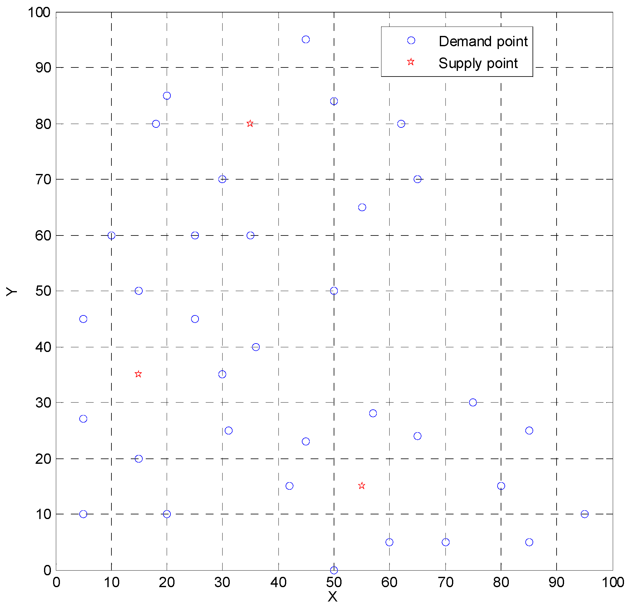
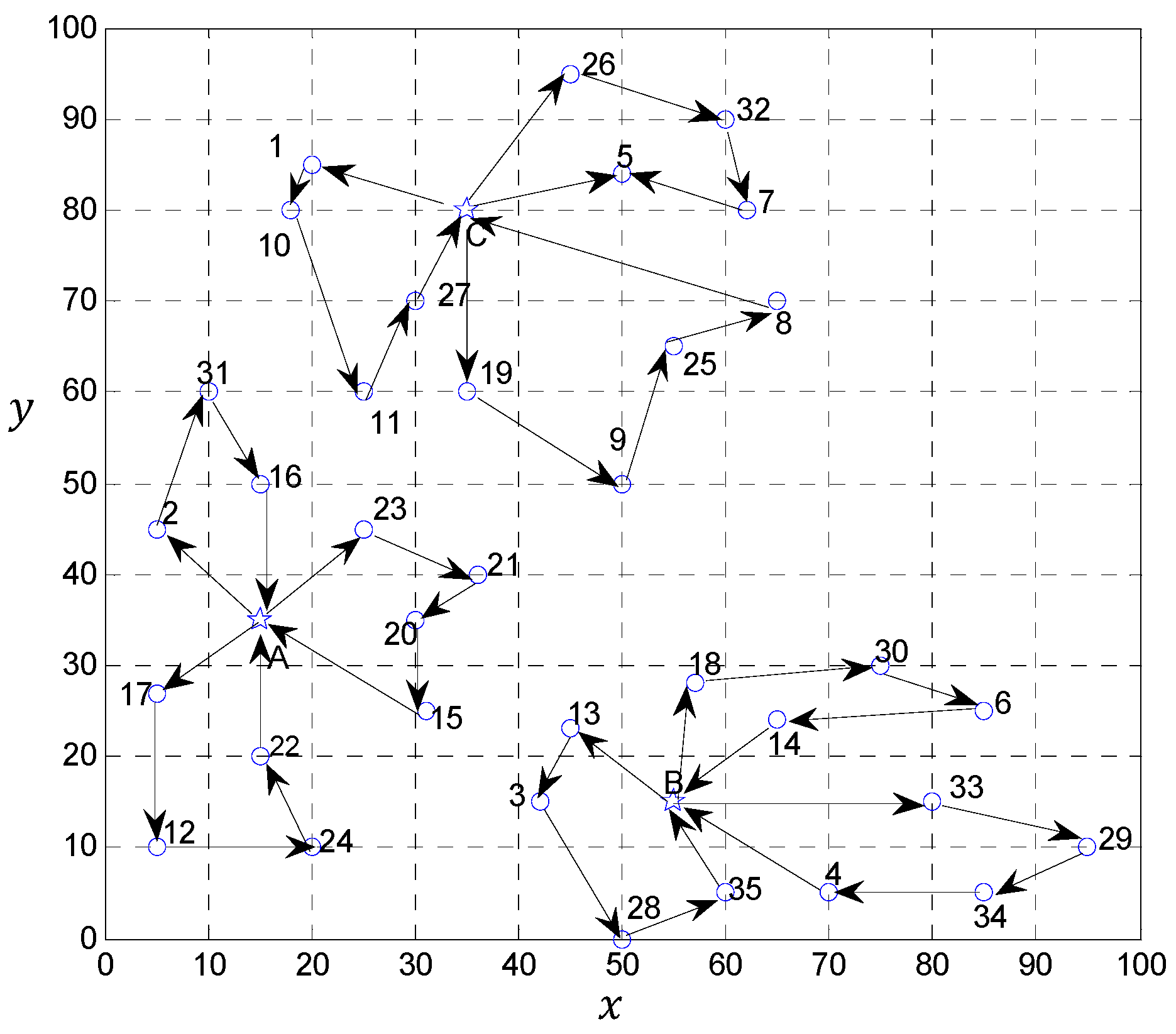
3.1. Numerical Example 1

A numerical example is presented in this section. The demand points and service centers are shown in Figure 1, in which there are three service centers (A, B, and C) and 35 demand points. The positions (represented as two-dimensional coordinate) of centers and the number of available vehicles in each center are given in

Table 2. Information of service centers.

Service Center	Coordinate (x, y)	Number of Available Vehicles
A	(15, 35)	5
B	(55, 15)	5
C	(35, 80)	5

.

In this example, we set the size of the population and maximum generation to be 50 and 1000, respectively. In addition, we assume that the emergency demand at each demand point follows normal distribution $N\left(\mu ,{\sigma }^2\right)$ within the given value interval, in which $\mu$ is the mean or expectation of the distribution, and $\sigma$ is its standard deviation with its variance as ${\sigma }^2$. Then, we know that:

$$f_k\left(x\right)=\frac{1}{\sqrt{2\pi }\sigma }exp\left(-\frac{{\left(x-\mu \right)}^2}{2{\sigma }^2}\right)$$

(23)

These parameters, including $\mu$, ${\sigma }^2$ and value interval, are shown in

Table 3. Information of demand points.

Demand Point	Coordinate (x, y)	Parameters ($\mathit{\mu },{\mathit{\sigma }}^2$)	Demand Interval (ton)	Time-Window (min)
1	(20, 85)	(5, 1.72)	[4, 6]	[0, 40]
2	(5, 45)	(5, 1.52)	[5, 7]	[0, 40]
3	(42, 15)	(8, 22)	[7, 10]	[0, 50]
4	(70, 5)	(7, 22)	[7, 9]	[0, 140]
5	(50, 84)	(6, 22)	[6, 8]	[0, 100]
6	(85, 25)	(9, 2.52)	[8, 11]	[0, 90]
7	(62, 80)	(6, 22)	[5, 7]	[0, 170]
8	(65, 70)	(4, 12)	[4, 5]	[0, 140]
9	(50, 50)	(11,3.52)	[10, 12]	[0, 85]
10	(18, 80)	(7, 22)	[7, 8]	[0, 50]
11	(25, 60)	(5, 1.52)	[4, 6]	[0, 90]
12	(5, 10)	(7, 22)	[7, 10]	[0, 105]
13	(45, 23)	(7, 22)	[5, 8]	[0, 50]
14	(65, 24)	(9, 32)	[8, 10]	[0, 130]
15	(31, 25)	(3, 12)	[3, 5]	[0, 90]
16	(15, 50)	(10, 32)	[10, 11]	[0, 85]
17	(5, 27)	(4, 12)	[4, 6]	[0, 70]
18	(57, 28)	(1, 0.32)	[1, 3]	[0, 40]
19	(35, 60)	(4, 12)	[4, 5]	[0, 45]
20	(30, 35)	(8, 22)	[8, 10]	[0, 100]
21	(36, 40)	(7, 22)	[7, 9]	[0, 90]
22	(15, 20)	(5, 1.62)	[5, 6]	[0, 165]
23	(25, 45)	(4, 1.32)	[4, 5]	[0, 110]
24	(20, 10)	(3, 12)	[3, 5]	[0, 135]
25	(55, 65)	(3, 12)	[3, 5]	[0, 115]
26	(45, 95)	(5, 1.52)	[5, 6]	[0, 45]
27	(30, 70)	(6, 22)	[6, 7]	[0, 115]
28	(50, 0)	(3, 0.92)	[2, 4]	[0, 85]
29	(95, 10)	(3, 0.92)	[2, 5]	[0, 90]
30	(75, 30)	(4, 1.32)	[4, 5]	[0, 80]
31	(10, 60)	(6, 1.92)	[6, 7]	[0, 90]
32	(60, 90)	(4, 1.32)	[4, 5]	[0, 80]
33	(80, 15)	(8, 2.52)	[8, 10]	[0, 60]
34	(85, 5)	(5, 1.62)	[5, 7]	[0, 115]
35	(60, 5)	(6, 22)	[6, 8]	[0, 120]

. The positions and the time windows that must be serviced for 35 demand points are also given in Table 3.

The number of available vehicles in centers is given by ${\vartheta }_1={\vartheta }_2={\vartheta }_3=5$, with the maximum load $Q=27$ ton and the average speed as 30 km/h. The fixed cost of vehicle per delivery is ${\omega }_v=200$ Yuan, $\forall v$. The transportation cost per kilometer is $c_{ij}=5$ Yuan/km, $\forall i,j$. When the delivered supplies do not meet the demand at the demand points, the penalty cost per supply unit for shortage at demand point is set as ${\phi }_k^{-}=500\mathrm{Yuan},\forall k$, and the penalty cost per supply unit for surplus at demand point is given by ${\phi }_k^{+}=300\mathrm{Yuan},\forall k$.

To transform the multi-depot problem into single-depot problem, the metrics of ratios and differences are valued as 0.65 and 22, respectively, in the Nearest Assignment method. The demand points with ratios less than 0.65 and differences more than 22 are chosen as boundary points. The results of the allocation according to the Nearest Allocation method are reported in

Table 4. Initial allocation of the demand points to service centers.

Set 1	Demand point	1	2	3	4	5	6	7	8	10	12
	Service Center	C	A	B	B	C	B	C	C	C	A
Set 2	Demand points	13	14	16	17	18	19	20	22	23	25
	Service Center	B	B	A	A	B	C	A	A	A	C
Set 3	Demand points	26	27	28	29	30	32	33	34	35
	Service Center	C	C	B	B	B	C	B	B	B

.

Based on the initial demand allocation results in Table 4, the Average Distance method is used to reallocate the boundary points, including demand points 9, 11, 15, 21, 24 and 31. The average distance between the each boundary point and the demand points in each set is calculated. The point should be inserted into the set in which the average distance is shortest. As a result, the final allocation is captured.

The initial solution is captured from random generation of initial population within each allocation set. Since the solution quality depends on the initial population in heuristic algorithm, ten computation tests are performed with different initial solutions. The proposed algorithm has been implemented in MATLAB and all the experimental tests were carried out on an Intel Pentium 3.20 GHz processor with 8GB of RAM (the same below). The maximum running time was limited to 12 s. The objective function values (OFV) of the corresponding ten optimal solutions are shown in Figure 2, where $\phi$ represents the OFV.

As demonstrated in Figure 2, the OFVs of the ten optimal solutions with different initial solutions are very close. In particular, the deviation between the maximum value (9789) and minimum value (9393) is only 4.21% different. Consequently, the solution method can be viewed to be convergent.

The convergence rate of the method is further described in Figure 3. We select the computation test with minimal OFV (9393) for the analysis. It can be found that the OFV decreases quickly with respect to the iteration of genetic algorithm. The optimal solution ($\phi =9393$) can be obtained at the 197th iteration, in which there are nine vehicles in three centers for the emergency supply delivery. The optimal allocation scheme and vehicle routes are reported/described in

Table 5. Vehicle routings and the actual service quantity.

Parking Lot	Route|Actual Amount	Route|Actual Amount	Route|Actual Amount
A	17-12-24-22|4.3-7.6-3.3-5.5	2-31-16|5.5-6.6-11.0	23-21-20-15|4.4-7.6-8.6-3.3
B	13-3-28-35|7.6-8.6-3.3-6.6	18-30-6-14|2.0-4.4-9.8-8.0	33-29-34-4|8.8-3.3-5.5-7.6
C	19-9-25-8|4.3-11.1-3.3-4.3	1-10-11-27|5.5-7.4-5.5-6.6	26-32-7-5|5.5-4.4-6.6-6.6

and Figure 4.

It is observed in the optimal solution that the number of used vehicles at each center and the serviced demand points of each center are almost equal respectively. For each center, there are 11 or 12 demand points which should be served and three vehicles are used to deliver supplies. For each vehicle, there are three or four demand points which should be delivered. In addition, the demand points with bigger time window, which have more flexibility, are always in the back of the vehicle routes. These features demonstrate that the results are rational.

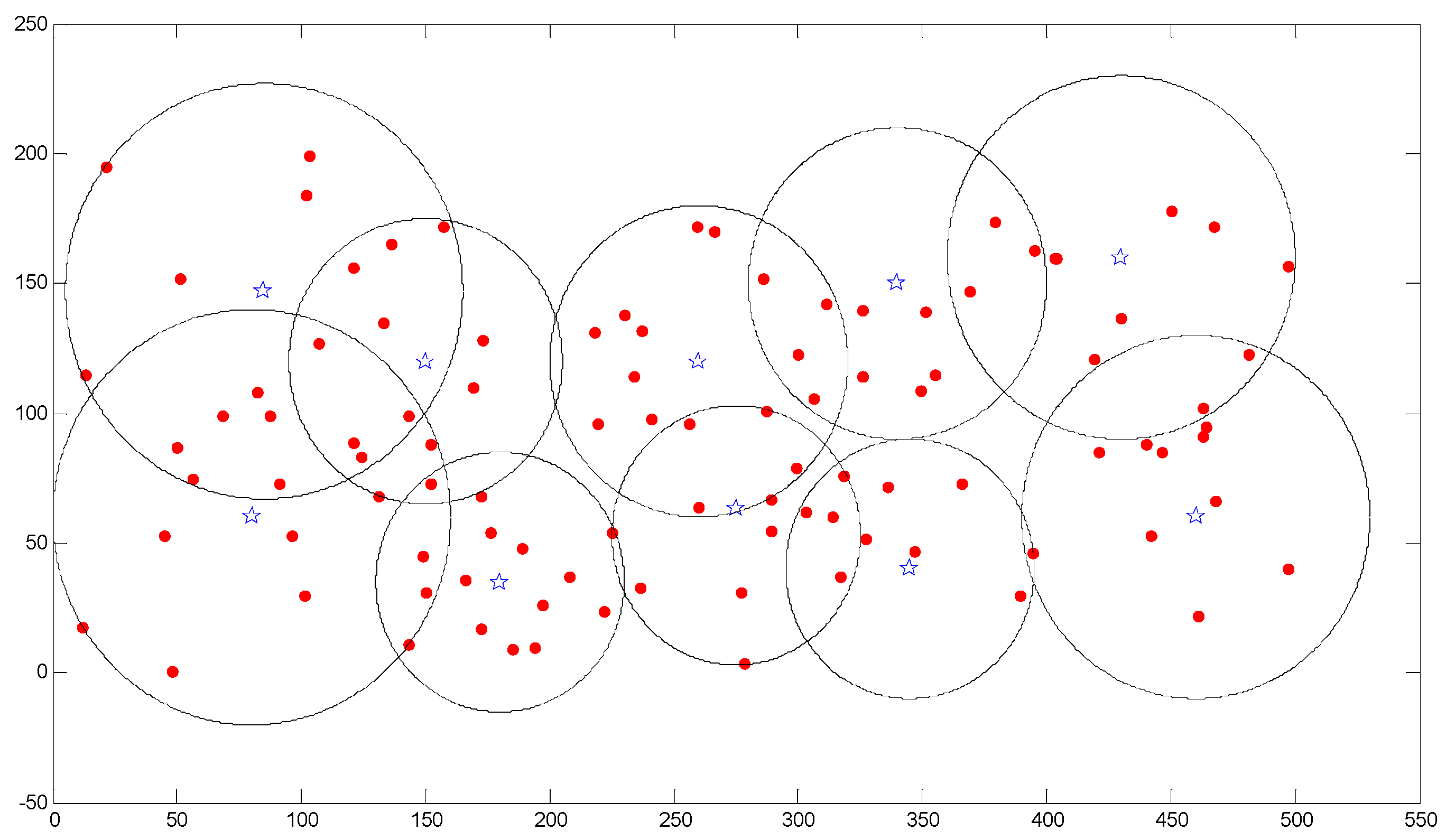
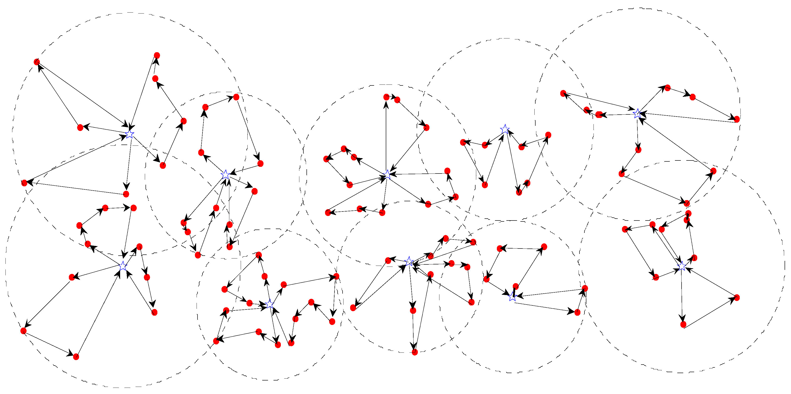
3.2. Numerical Example 2

Taking the waterlogging disaster in Changsha City of Hunan Province as an example, in Figure 5, the red dots and the blue dots represent the demand points and the supply points, respectively. The demand points and supply points in urban area are marked into coordinate axes. The specific data can be found in the Appendix A

Table A1. Information of service centers.

Service Center	Coordinate (x, y)	Number of Available Vehicles
1	(180, 35)	5
2	(275, 63)	6
3	(80, 60)	5
4	(85, 147)	6
5	(460, 60)	5
6	(430, 160)	5
7	(260, 120)	6
8	(345, 40)	4
9	(150, 120)	6
10	(340, 150)	4

and

Table A2. Information of demand points.

Demand Point	Coordinate (x, y)	Parameters ($\mathit{\mu },{\mathit{\sigma }}^2$)	Demand Interval (ton)	Time-Window (min)
1	(237, 132)	(7, 1.52)	[7, 9]	[0, 40]
2	(103, 199)	(6, 1.32)	[5, 7]	[0, 180]
3	(421, 85)	(11, 22)	[10, 12]	[0, 100]
4	(303, 62)	(7, 22)	[7, 9]	[0, 50]
5	(166, 36)	(9, 22)	[8, 12]	[0, 125]
6	(351, 139)	(6, 1.52)	[6, 8]	[0, 170]
7	(314, 60)	(8, 22)	[7, 9]	[0, 65]
8	(121, 89)	(7, 12)	[6, 9]	[0, 70]
9	(299, 79)	(11,2.52)	[10, 12]	[0, 55]
10	(450, 178)	(10, 22)	[9, 12]	[0, 40]
11	(366, 73)	(5, 1.52)	[4, 6]	[0, 50]
12	(317, 37)	(10, 22)	[9, 11]	[0, 110]
13	(102, 184)	(7, 22)	[5, 8]	[0, 160]
14	(48, 1)	(9, 32)	[8, 10]	[0, 200]
15	(287, 101)	(8, 12)	[7, 9]	[0, 60]
16	(157, 172)	(4, 12)	[4, 5]	[0, 125]
17	(442, 53)	(9, 12)	[8, 11]	[0, 160]
18	(241, 98)	(11, 1.32)	[10, 13]	[0, 65]
19	(169, 110)	(11, 22)	[10, 13]	[0, 45]
20	(197, 26)	(5, 1.42)	[5, 6]	[0, 200]
21	(327, 52)	(9, 22)	[8, 10]	[0, 140]
22	(131, 68)	(8, 1.22)	[7, 9]	[0, 120]
23	(481, 123)	(7, 1.32)	[6, 8]	[0, 180]
24	(395, 163)	(6, 12)	[5, 7]	[0, 65]
25	(50, 87)	(7, 1.42)	[6, 9]	[0, 70]
26	(278, 4)	(9, 1.52)	[8, 10]	[0, 85]
27	(208, 37)	(5, 1.22)	[5, 7]	[0, 125]
28	(133, 135)	(6, 0.92)	[5, 7]	[0, 40]
29	(230, 138)	(5, 0.92)	[4, 6]	[0, 60]
30	(101, 30)	(8, 1.32)	[6, 9]	[0, 85]
31	(349, 109)	(8, 1.92)	[7, 9]	[0, 60]
32	(12, 18)	(9, 1.32)	[8, 11]	[0, 120]
33	(87, 99)	(8, 2.52)	[8, 10]	[0, 130]
34	(318, 76)	(11, 1.62)	[10, 13]	[0, 90]
35	(326, 140)	(6, 22)	[5, 7]	[0, 40]
36	(369, 147)	(7, 1.32)	[7, 10]	[0, 130]
37	(336, 72)	(6, 1.22)	[5, 8]	[0, 100]
38	(21, 195)	(13, 2.52)	[12, 15]	[0, 130]
39	(497, 40)	(12, 1.62)	[11, 14]	[0, 120]
40	(149, 45)	(6, 22)	[5, 8]	[0, 100]
41	(403, 160)	(5, 1.22)	[5, 7]	[0, 45]
42	(91, 73)	(10, 22)	[9, 11]	[0, 40]
43	(236, 33)	(14, 2.52)	[13, 15]	[0, 80]
44	(256, 96)	(9, 1.92)	[8, 11]	[0, 45]
45	(464, 95)	(10, 1.32)	[9, 12]	[0, 50]
46	(277, 31)	(8, 22)	[8, 10]	[0, 45]
47	(260, 64)	(11, 22)	[10, 13]	[0, 35]
48	(194, 10)	(5, 1.22)	[4, 6]	[0, 230]
49	(96, 53)	(8, 22)	[7, 10]	[0, 70]
50	(218, 131)	(8, 1.52)	[8, 10]	[0, 90]
51	(124, 83)	(8, 1.92)	[8, 10]	[0, 85]
52	(225, 54)	(4, 1.12)	[3, 5]	[0, 80]
53	(463, 102)	(5, 22)	[5, 7]	[0, 140]
54	(176, 54)	(5, 0.92)	[4, 6]	[0, 30]
55	(497, 157)	(8, 1.72)	[7, 9]	[0, 120]
56	(389, 30)	(15, 2.32)	[14, 17]	[0, 70]
57	(440, 88)	(7, 1.92)	[6, 8]	[0, 50]
58	(300, 123)	(10, 1.32)	[9, 12]	[0, 115]
59	(51, 152)	(12, 22)	[10,15]	[0, 60]
60	(463, 91)	(6, 1.62)	[5, 7]	[0, 40]
61	(143, 99)	(6, 22)	[5, 7]	[0, 170]
62	(152, 88)	(10, 1.32)	[9, 12]	[0, 130]
63	(219, 96)	(6, 1.22)	[6, 8]	[0, 110]
64	(446, 85)	(5, 1.62)	[5, 7]	[0, 85]
65	(289, 55)	(9, 22)	[9, 11]	[0, 160]
66	(152, 73)	(6, 22)	[5, 7]	[0, 100]
67	(13, 115)	(15, 32)	[14, 17]	[0, 160]
68	(430, 137)	(6, 1.62)	[6, 7]	[0, 40]
69	(467, 172)	(9, 22)	[8, 10]	[0, 70]
70	(289, 67)	(6, 1.22)	[6, 8]	[0, 35]
71	(172, 17)	(7, 1.22)	[6, 8]	[0, 70]
72	(121, 156)	(7, 1.22)	[6, 8]	[0, 90]
73	(82, 108)	(9, 1.52)	[8, 10]	[0, 60]
74	(326, 114)	(12, 1.92)	[10, 14]	[0, 120]
75	(107, 127)	(7, 1.32)	[6, 8]	[0, 45]
76	(189, 48)	(3, 0.82)	[3, 4]	[0, 30]
77	(355, 115)	(7, 1.62)	[6, 8]	[0, 80]
78	(286, 152)	(10, 22)	[9, 12]	[0, 140]
79	(306, 106)	(7, 1.32)	[7, 8]	[0, 90]
80	(185, 9)	(8, 1.42)	[7, 10]	[0, 45]
81	(45, 53)	(10, 22)	[10, 12]	[0, 60]
82	(468, 66)	(6, 1.52)	[6, 8]	[0, 30]
83	(419, 121)	(7, 1.92)	[6, 8]	[0, 70]
84	(461, 22)	(14, 2.32)	[12, 16]	[0, 60]
85	(172, 68)	(7, 22)	[6, 9]	[0, 60]
86	(173, 128)	(7, 1.62)	[8, 10]	[0, 185]
87	(150, 31)	(9, 22)	[9, 11]	[0, 145]
88	(347, 47)	(7, 1.62)	[6, 8]	[0, 30]
89	(379, 174)	(7, 1.42)	[7, 10]	[0, 100]
90	(56, 75)	(7, 1.32)	[5, 8]	[0, 50]
91	(394, 46)	(12, 22)	[11, 14]	[0, 100]
92	(136, 165)	(8, 1.52)	[7, 9]	[0, 85]
93	(259, 172)	(7, 1.92)	[6, 9]	[0, 80]
94	(143, 11)	(3, 0.82)	[3, 4]	[0, 115]
95	(68, 99)	(6, 1.92)	[5, 8]	[0, 100]
96	(311, 142)	(8, 1.32)	[8, 10]	[0, 70]
97	(234, 114)	(7, 2.52)	[7, 8]	[0, 130]
98	(266, 170)	(8, 1.62)	[8, 11]	[0, 100]
99	(222, 24)	(3, 12)	[3, 4]	[0, 120]
100	(404, 160)	(8, 22)	[7, 10]	[0, 50]

. The maximum load of vehicles is $Q=30$ ton and the average speed as 40 km/h. The fixed cost of vehicle per delivery is ${\omega }_v=200$ Yuan, $\forall v$. The transportation cost per kilometer is $c_{ij}=3$ Yuan/km, $\forall i,j$. When the delivered supplies do not meet the demand at the demand points, the penalty cost per supply unit for shortage at demand point is set as ${\phi }_k^{-}=100\mathrm{Yuan},\forall k$, and the penalty cost per supply unit for surplus at demand point is given by ${\phi }_k^{+}=60\mathrm{Yuan},\forall k$.

According to the method described in Section 2.3, we obtain the radius of the emergency service of each supply point. Then we determine the served demand point set of each supply center, as shown in Figure 6, which depicts the covered demand point within the scope of the emergency service by each demand point. The results of the allocation according to the Nearest Allocation method are reported as Appendix A

Table A3. Allocation of the demand points to service centers.

Service Center	Demand Points
1	5,20,27,40,48,52,54,71,76,80,85,87,94,99
2	4,7,9,12,26,34,43,46,47,65,70
3	14,25,30,32,33,42,49,81,90,95
4	2,13,38,59,67,72,73,75
5	3,17,39,45,57,60,64,82,84
6	10,23,24,41,53,55,68,69,83,89,100
7	1,15,18,29,44,50,58,63,78,79,93,97,98
8	11,21,37,56,88,91
9	8,16,19,22,28,51,61,62,66,86,92
10	6,31,35,36,74,77,96

.

In this example, ten computation tests are performed with different initial solutions. The computation of the proposed algorithm is implemented in MATLAB. The maximum running time was less than 18 s. The optimal allocation scheme and vehicle routes are described in Figure 7. It is observed that the total traveled distance is 3713.9, and the total cost equals 18,217.7.

From the data in

Table 6. The initial solutions vs. the optimal solutions.

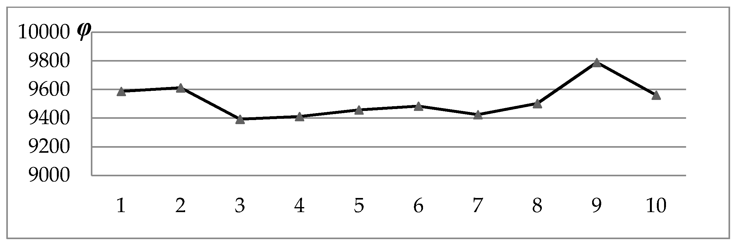
Number	OFV of Initial Solution	OFV of Optimal Solution	Relative Cost Savings/%	Operation Time/s
1	23,077.8	18,736.2	18.78	22.73
2	22,978.3	19,010.8	17.27	21.64
3	22,621.5	18,708.2	17.30	21.77
4	23,103.7	19,087.6	17.38	21.34
5	21,785.5	18,217.7	16.38	22.19
6	21,952.6	18,438.0	16.01	21.69
7	22,372.4	18,217.7	18.57	23.73
8	23,189.2	19,128.4	17.12	21.80
9	22,478.3	18,394.1	18.17	21.87
10	23,296.7	18,747.5	19.52	23.05

, we can see, in the premise of different initial solutions, the total costs of 10 calculation optimal solutions is very close through MRGA algorithm, the relative deviation is only 4.7% to the maximum value (19,128.4) and the minimum value (18,217.7); in comparison with the initial solution, the use of MRGA algorithm to solve the problem has saved 16.01%–19.52%, and the computation time, mostly being within 24 s, also proved the efficiency of the proposed optimization model and MRGA algorithm.

Similar to example 1, the number of used vehicles at each center and the serviced demand points of each center are almost equal respectively. In most cases, there are 8–14 demand points which should be delivered by three vehicles. For each vehicle, there are almost three or four demand points which should be delivered except for a few vehicles services for two demand points and only one vehicle service for six demand points. In demand intensive areas, one vehicle could serve for more demand points, while a vehicle could provide emergency resources for two demand points at most in the remote area, where the demand is not concentrated. In general, the demand points with bigger time window are always behind the vehicle routes. The instance indicates that the proposed algorithm for the emergency vehicle routing problem is reasonable and efficient.

In

Table 7. Total cost and Distance vs. The penalty costs.

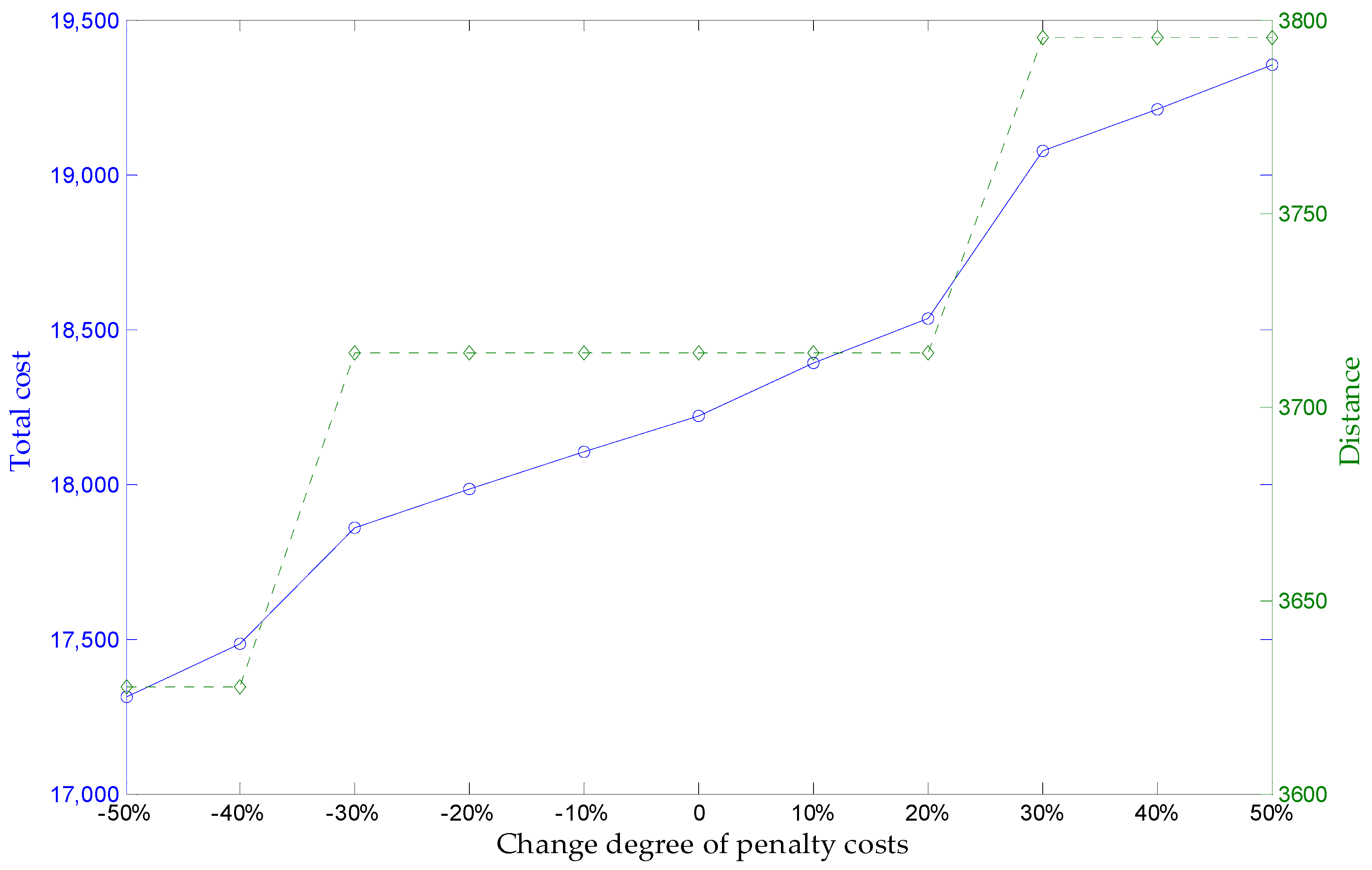
Variation Range	Number of Used Vehicles on Each Demands Points (in Order of Service Center)	Total Cost	Distance
−50%	[3,3,2,2,3,3,3,2,3,2]	17,314.6	3627.5
−40%	[3,3,2,2,3,3,4,2,3,2]	17,482.7	3627.5
−30%	[3,4,3,3,3,3,4,2,3,2]	17,859.2	3713.9
−20%	[3,4,3,3,3,3,4,2,3,2]	17,985.5	3713.9
−10%	[3,4,3,3,3,3,4,2,3,2]	18,102.4	3713.9
0	[3,4,3,3,3,3,4,2,3,2]	18,217.7	3713.9
10%	[3,4,3,3,3,3,4,2,3,2]	18,391.5	3713.9
20%	[3,4,3,3,3,3,4,2,3,2]	18,533.9	3713.9
30%	[4,4,3,3,3,3,4,2,3,3]	19,074.2	3795.4
40%	[4,4,3,3,3,3,4,2,3,3]	19,208.6	3795.4
50%	[4,4,3,3,3,3,4,2,3,3]	19,352.3	3795.4

, we change the penalty costs ${\phi }_k^{-}$ and ${\phi }_k^{+}$, and keep other parameters unchanged; five experiments are carried out for each degree and we take the average as a result. With the increase of penalty cost, the total cost of the system increases, on the contrary; the total cost of the system decreases with the decrease of penalty cost. In the range of more than 20% increase, the number of used vehicles on several demands points increase as well; on the other hand, the results remain unchanged in the case of reducing the penalty costs in the range of 30%; with the increase rate up to 40%, the number of used vehicles on several demands points decrease. As depicted in the Figure 8, the evolution trend between total cost and distance is very closely. In the range [−30%, 20%], the distance remain unchanged, as the total cost close to linear change and change slowly; while the change degree reaches −40% and 30%, the distance present a variation with a jump, as does the total cost.

Next, we change the time windows while keeping other parameters unchanged (it is assumed that all time windows in the system are changed at the same rate). With the increase of time windows, the results remain unchanged; on the contrary, the total cost and distance of the system increase with the decrease of time windows. In the range of more than 10% decrease, the number of used vehicles on several demands points increase; on the other hand, the results remain unchanged in the case of raising the time windows; when the change rate runs up to 50%, there are no feasible solutions in several demands points. The specific data are in

Table 8. Total cost and Distance vs. The time windows.

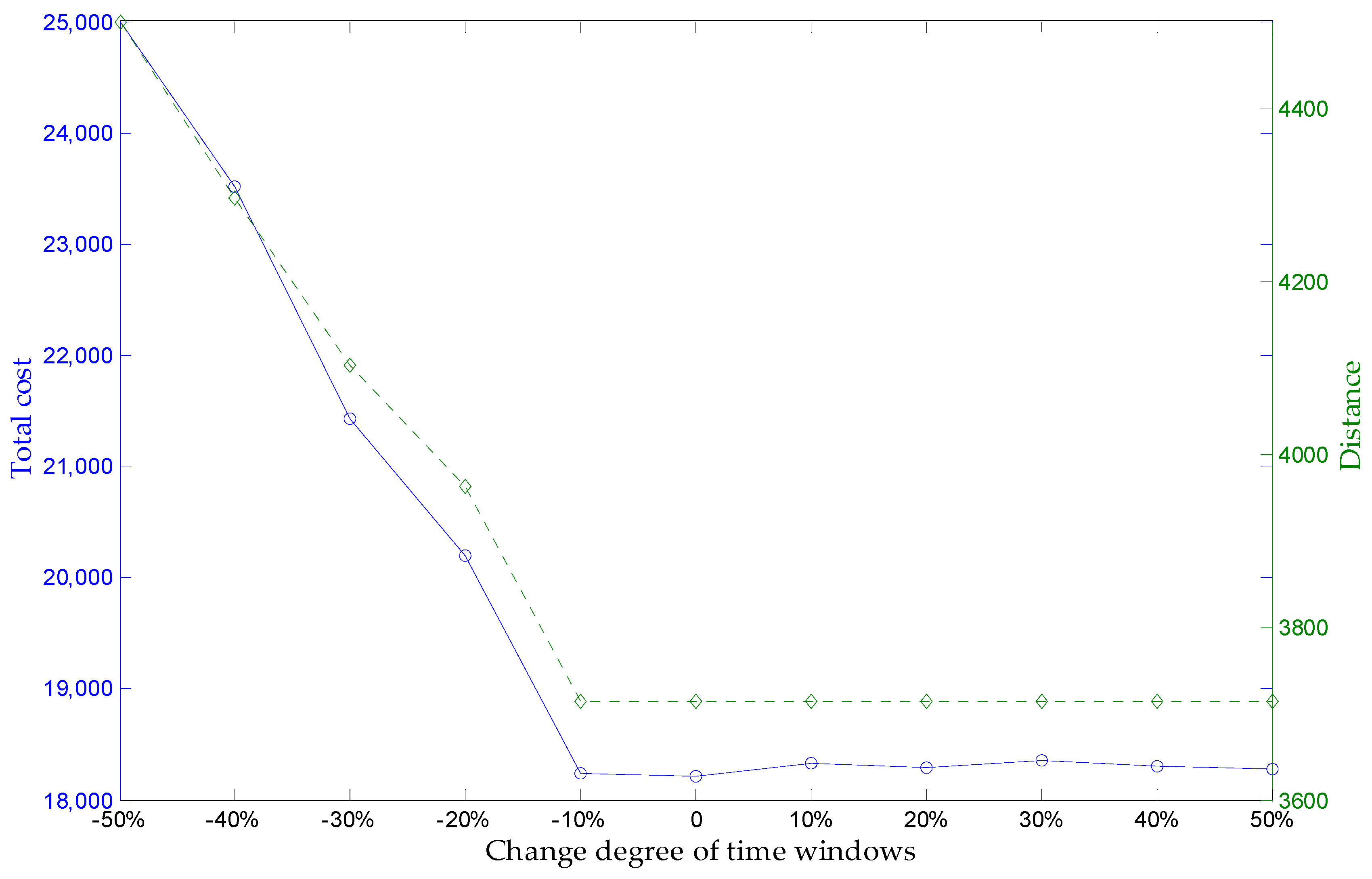
Variation Range	Number of Used Vehicles on Each Demands Points(in Order of Service Center)	Total Cost	Distance
−50%	[-,6,5,5,5,5,-,4,-,4]
−40%	[5,5,4,4,4,5,6,3,5,4]	23,509.7	4296.5
−30%	[4,5,3,4,3,4,5,3,4,3]	21,430.2	4101.9
−20%	[4,4,3,4,3,4,4,2,4,3]	20,193.6	3962.9
−10%	[3,4,3,3,3,3,4,2,3,2]	18,241.4	3713.9
0	[3,4,3,3,3,3,4,2,3,2]	18,217.7	3713.9
10%	[3,4,3,3,3,3,4,2,3,2]	18,330.5	3713.9
20%	[3,4,3,3,3,3,4,2,3,2]	18,293.1	3713.9
30%	[3,4,3,3,3,3,4,2,3,2]	18,351.2	3713.9
40%	[3,4,3,3,3,3,4,2,3,2]	18,308.6	3713.9
50%	[3,4,3,3,3,3,4,2,3,2]	18,276.3	3713.9

. In addition, we can see from Figure 9 that the trend of change in cost and distance are consistent.

3.3. Comparison with Other Metaheuristics

A computational experiment has been conducted to compare the performance of the proposed algorithm with some of the best techniques designed recently for VRPTW. The improved Genetic Algorithm of the proposed problem has been tested with 56 VRPTW benchmark problems of Solomon. Each problem is involved with 100 customers, randomly distributed over a geographical area except for different the demands, while the emergency demand at each demand point follows normal distribution $N\left(\mu ,{\sigma }^2\right)$ (see Formula (23)), within the given data as the center to set up the demand interval. In this article, the value of $\mu$ is set to be the demand amount at each demand point in the VRPTW benchmark problems, with the value of ${\sigma }^2$ as 2²; by setting $\mu$ as the center, we pick two nearest integers, one to the left, one to the right of $\mu$, and establish a demand interval by taking these two integers as the boundary points. For example, if the demand amount value is 10 at one demand point, we take $\mu$ as 10, and the corresponding demand interval turns out to be (9,11).

The parameter values for the problems are described below: In fitness and objective functions, the maximum load $Q=200$; the average speed is 30 and the fixed cost of vehicle per delivery is ${\omega }_v=300$, $\forall v$. The transportation cost per unit is $c_{ij}=5$, $\forall i,j$. When the delivered supplies do not meet the demand at the demand points, the penalty cost per supply unit for shortage at demand point is ${\phi }_k^{-}=100,$ and the penalty cost per supply unit for surplus at demand point is ${\phi }_k^{+}=50,\forall k$.

The probabilities and parameter values for the proposed genetic operators are defined as follows: The population size and maximum generation size are equal to 20 and 1000, respectively. The parameter values of selection, crossover and mutation operators can be calculated through the above Equations (20)–(22), respectively.

The proposed algorithm has been implemented in MATLAB and the experimental tests were carried out on an Intel Pentium 3.20 GHz processor with 8 GB of RAM. The maximum running time was limited to 100 s and the experiment consisted of performing five simulation runs for each problem instance in a given data set.

This is justified by the fact that the sensitivity of the results with respect to changes in the parameter values, such as recombination and mutation rates, was found to be generally quite small. When we change the population size from 20 to 30 and 50, the corresponding difference of results is quite small but the running time becomes a little shorter; when the parameter values of selection, crossover and mutation operators are modified in a reasonable range, the results do not indicate obvious differences.

The results for the six problem data sets are summarized in

Table 9. The performance of the proposed method.

Problem		Average Performance	Best Performance
R1	Cost	15,697.13	14,746.00
	Distance	1239.53	1234.39
	Vehicles	13.08	13.08
R2	Cost	11,475.46	11,293.00
	Distance	911.99	907.51
	Vehicles	4.45	4.45
C1	Cost	12,904.28	12,859.00
	Distance	829.29	828.50
	Vehicles	10.00	10.00
C2	Cost	9558.90	9426.00
	Distance	593.87	589.86
	Vehicles	3.25	3.25
RC1	Cost	16,257.74	15,948.00
	Distance	1384.44	1381.56
	Vehicles	12.75	12.75
RC2	Cost	12,632.35	12,315.00
	Distance	1041.74	1038.95
	Vehicles	5.25	5.25

, and the detailed data can be found in Appendix A

Table A4. The performance of the proposed method to the problem (Solomon Benchmarks with narrow time windows).

Instance Data	Distance	Vehicles	Instance Data	Distance	Vehicles	Instance Data	Distance	Vehicles
R101	1683.8	20	C101	828.94	10	RC101	1675.86	15
R102	1526.75	18	C102	828.94	10	RC102	1488.36	14
R103	1319.12	14	C103	828.06	10	RC103	1306.42	12
R104	1097.63	11	C104	825.65	10	RC104	1145.79	10
R105	1415.24	15	C105	828.94	10	RC105	1608.45	15
R106	1275.58	13	C106	828.94	10	RC106	1408.70	13
R107	1104.76	11	C107	830.56	10	RC107	1254.26	12
R108	1008.9	10	C108	834.62	10	RC108	1187.53	11
R109	1187.3	13	C109	828.94	10
R110	1142.4	11
R111	1129.72	11
R112	982.14	10

and

Table A5. The performance of the proposed method to the problem (Solomon Benchmarks with wide time windows).

Instance Data	Distance	Vehicles	Instance Data	Distance	Vehicles	Instance Data	Distance	Vehicles
R201	1206.27	6	C201	591.56	3	RC201	1357.35	7
R202	1046.16	5	C202	608.39	4	RC202	1167.1	6
R203	890.50	5	C203	591.17	3	RC203	951.08	5
R204	767.92	3	C204	596.55	3	RC204	796.14	4
R205	975.83	5	C205	588.88	3	RC205	1209.83	6
R206	900.42	4	C206	588.49	3	RC206	1080.50	5
R207	847.57	3	C207	597.61	4	RC207	985.56	5
R208	738.41	5	C208	588.32	3	RC208	785.93	4
R209	885.64	5
R210	931.78	5
R211	841.39	3

. The results are expressed according to objective function, where the cost is considered as the primary factor and, for the particularity and practicality of emergency rescue after disaster, the total traveled distance or total duration of routes is also considered. In addition, the number of vehicles is demonstrated in the results, so that the sustainability of emergency service is satisfied.

The genetic algorithm described above is compared in

Table 10. Average performance comparison among other metaheuristics.

Problem		BBB	M	RT	JM	HG	BC	BD	QYC
R1	Distance	1251.40	1208	1208.50	1179.95	1212.73	1209.19	1220.14	1239.53
	Vehicles	12.17	12.00	12.25	13.25	11.92	12.08	12.00	13.08
R2	Distance	1056.59	954	961.72	878.41	955.03	963.62	977.57	911.99
	Vehicles	2.73	2.73	2.91	5.36	2.73	2.73	2.73	4.45
C1	Distance	828.50	829	828.38	828.38	828.38	828.38	828.38	829.29
	Vehicles	10.00	10.00	10.00	10.00	10.00	10.00	10.00	10.00
C2	Distance	590.06	590	589.86	589.86	589.86	589.86	589.86	593.87
	Vehicles	3.00	3.00	3.00	3.00	3.00	3.00	3.00	3.25
RC1	Distance	1414.86	1387	1377.39	1343.64	1386.44	1389.22	1397.44	1384.44
	Vehicles	11.88	11.50	11.88	13.00	11.50	11.50	11.50	12.75
RC2	Distance	1258.15	1119	1119.59	1004.21	1123.17	1143.70	1140.06	1041.74
	Vehicles	3.25	3.25	3.38	6.25	3.25	3.25	3.25	5.25
Time(min)		Pentium 400 MHz, 30 min	Pentium III 450 MHz, 150.2 min	Silicon Graphics 100 MHz	Pentium III 1 GHz, 0.8 min	Pentium 400 MHz, --	5 × Pentium 850 MHz, 12 min	AMD 700 Mz, 9.1 min	Pentium 3.20 GHz, 1.7 min

with some of the other classical metaheuristics [40,41] by Berger, Barkaoui, and Braysy (BBB,2003); Mester (M,2002); Rochat and Taillard (RT,1995); Jung and Moon (JM,2002); Homberger and Gehring (HG,2005); Bouthillier and Crainic (BC,2005); and Braysy and Dullaert (BD,2003). The rightmost column describes the results of our proposed method, including total traveled distance and the number of vehicles, the computer and the CPU time are also described as reported by the authors.

According to Table 10, the results of those experiments do not indicate any conclusive evidence to support a dominating heuristic over the others. Due to the difference and uncertainty of the emergency demand interval, the problem relative to the previous examples has increased its complexity, but, in general, the results by the proposed method prove to be competitive and effective, since it is the closest to the performance of best-known heuristic routing procedures. Moreover, it is demonstrated that the emergency vehicle routing problem can be tested through the VRPTW benchmark problems of Solomon in an acceptable way.

4. Conclusions

To improve sustainability of rescue operation after disaster, utilizing limited emergency resource reasonably was required. In this paper, the emergency VRP with insufficient supplies and uncertain demands during the crucial rescue period (the initial 72-h) after the disaster were investigated, hoping to enhance timeliness, utilization and sustainability of the emergency service. Combined with the characteristics of the crucial rescue period, such as the emergency resources are always limited, the uncertain emergence demands following the probability distribution is assumed at first. Based on this assumption, the expected penalty costs are incurred by the decision of resource distribution, due to the shortage and surplus of the relief supplies at each demand point. Then, the optimization model for emergency vehicles routing problem with insufficient supplies is proposed, in which the objective function was to minimize the transportation costs, vehicle operation costs and the penalty costs at all demand points.

The problem was divided into two steps. In first step, the Nearest Assignment method and Average Distance method were used to transform the multi-depot vehicle routing problem into multiple single-depot vehicle routing problem; meanwhile, the service point set of each service center was determined. Then, the heuristics algorithm, based on Genetic Algorithm (GA), was developed to solve the single-depot vehicle routing problems. In order to improve solution quality and efficiency, the hybrid encoding mode was used to construct genetic operator in the algorithm.

The numerical example demonstrated that the presented method would address the problem quickly and efficiently. The results illuminated that the model performed well in the disaster rescue operation, where appropriate amount delivery was momentous because only correct deliveries of supplies could make sure to keep the people in the affected area alive as long as possible and to wait for the subsequent rescue. In addition, our model was sensitive to the penalty cost settings, and this fact suggests that rational determinations of the penalty cost would make our model more efficient.

Many variants of the proposed model could be considered in the future research; for instance, a penalty for missing the time window could be introduced, different types of resources could be appropriately defined, etc. Further research could be carried out related to the proposed parameters and their performance. Moreover, applications of the proposed concept of penalty to other related problems are also possible in the sustainability environments.

References

- Caunhye, A.M.; Nie, X.F.; Pokharel, S. Optimization models in emergency logistics: A literature review. Socio-Econ. Plan. Sci. 2012, 46, 4–13. [Google Scholar] [CrossRef]
- Lin, Y.H.; Batta, R.; Rogerson, P.A.; Blatt, A.; Flanigan, M. A logistics model for emergency supply of critical items in the aftermath of a disaster. Socio-Econ. Plan. Sci. 2011, 45, 132–145. [Google Scholar] [CrossRef]
- Sheu, J.B. Challenges of emergency logistics management. Transp. Res. Part E Logist. Transp. Rev. 2007, 43, 655–659. [Google Scholar] [CrossRef]
- Sheu, J.B. An emergency logistics distribution approach for quick response to urgent relief demand in disasters. Transp. Res. Part E Logist. Transp. Rev. 2007, 43, 687–709. [Google Scholar] [CrossRef]
- Lei, H.T.; Laporte, G.; Guo, B. The capacitated vehicle routing problem with stochastic demands and time windows. Comput. Oper. Res. 2011, 38, 1775–1783. [Google Scholar] [CrossRef]
- Zhu, L.; Rousseau, L.M.; Rei, W.; Li, B. Paired cooperative reoptimization strategy for the vehicle routing problem with stochastic demands. Comput. Oper. Res. 2014, 50, 1–13. [Google Scholar] [CrossRef]
- Errico, F.; Desaulniers, G.; Gendreau, M.; Rei, W.; Rousseau, L.M. A priori optimization with recourse for the vehicle routing problem with hard time windows and stochastic service times. Eur. J. Oper. Res. 2016, 249, 55–66. [Google Scholar] [CrossRef]
- Zhang, J.L.; Lam, W.H.K.; Chen, B.Y. On-time delivery probabilistic models for the vehicle routing problem with stochastic demands and time windows. Eur. J. Oper. Res. 2016, 249, 144–154. [Google Scholar] [CrossRef]
- Yin, P.Y.; Chuang, Y.L. Adaptive Memory Artificial Bee Colony Algorithm for Green Vehicle Routing with Cross-Docking. Appl. Math. Model. 2016, 40, 9302–9315. [Google Scholar] [CrossRef]
- Yin, P.Y.; Lyu, S.R.; Chuang, Y.L. Cooperative Coevolutionary Approach for Integrated Vehicle Routing and Scheduling Using Cross-Dock Buffering. Eng. Appl. Artif. Intell. 2016, 52, 40–53. [Google Scholar] [CrossRef]
- Marinakis, Y.; Iordanidou, G.R.; Marinaki, M. Particle swarm optimization for the vehicle routing problem with stochastic demands. Appl. Soft Comput. 2013, 13, 1693–1704. [Google Scholar] [CrossRef]
- Euchi, J.; Chabchoub, H.; Yassine, A. New Evolutionary Algorithm Based on 2-Opt Local Search to Solve the Vehicle Routing Problem with Private Fleet and Common Carrier. Int. J. Appl. Metaheuristic Comput 2011, 2, 58–82. [Google Scholar] [CrossRef]
- Parragh, S.N.; Doerner, K.F.; Hartl, R.F. A survey on pickup and delivery problems: Part I: Transportation between customers and depot. J. Betriebswirtsch. 2008, 58, 21–51. [Google Scholar] [CrossRef]
- Parragh, S.N.; Doerner, K.F.; Hartl, R.F. A survey on pickup and delivery problems: Part II: Transportation between pickup and delivery locations. J. Betriebswirtsch. 2008, 58, 81–117. [Google Scholar] [CrossRef]
- Berghida, M.; Boukra, A.; Boumedienne, H. Resolution of a Vehicle Routing Problem with Simultaneous Pickup and Delivery: A Cooperative Approach. Int. J. Appl. Metaheuristic Comput. 2015, 6, 53–68. [Google Scholar] [CrossRef]
- Maquera, G.; Laguna, M.; Gandelman, D.; Sant’Anna, A. Scatter Search Applied to the Vehicle Routing Problem with Simultaneous Delivery and Pickup. Int. J. Appl. Metaheuristic Comput. 2011, 2, 1–20. [Google Scholar] [CrossRef]
- Wohlgemuth, S.; Oloruntoba, R.; Clausen, U. Dynamic vehicle routing with anticipation in disaster relief. Socio-Econ. Plan. Sci. 2012, 46, 261–271. [Google Scholar] [CrossRef]
- Pillac, V.; Gendreau, M.; Guéret, C.; Medaglia, A.L. A review of dynamic vehicle routing problems. Eur. J. Oper. Res. 2013, 225, 1–11. [Google Scholar] [CrossRef] [Green Version]
- Cao, E.; Lai, M.Y.; Yang, H.M. Open vehicle routing problem with demand uncertainty and its robust strategies. Expert Syst. Appl. 2014, 41, 3569–3575. [Google Scholar] [CrossRef]
- Moghaddama, B.F.; Ruiz, R.; Sadjadi, S.J. Vehicle routing problem with uncertain demands: An advanced particle swarm algorithm. Comput. Ind. Eng. 2012, 62, 306–317. [Google Scholar] [CrossRef]
- Sheu, J.B. Dynamic relief-demand management for emergency logistics operations under large-scale disasters. Transp. Res. Part E Logist. Transp. Rev. 2010, 46, 1–17. [Google Scholar] [CrossRef]
- Chang, F.S.; Wu, J.S.; Lee, C.N.; Shen, H.C. Greedy-search-based multi-objective genetic algorithm for emergency logistics scheduling. Expert Syst. Appl. 2014, 41, 2947–2956. [Google Scholar] [CrossRef]
- Wang, H.J.; Du, L.J.; Ma, S.H. Multi-objective open location-routing model with split delivery for optimized relief distribution in post-earthquake. Transp. Res. Part E Logist. Transp. Rev. 2014, 69, 160–179. [Google Scholar] [CrossRef]
- Hochbaum, D.S.; Shmoys, D.B. Best possible heuristics for the bottleneck wandering salesperson and bottleneck vehicle routing problem. Eur. J. Oper. Res. 1986, 26, 380–384. [Google Scholar] [CrossRef]
- Ombuki, B.; Ross, B.J.; Hanshar, F. Multi-objective genetic algorithms for vehicle routing problem with time windows. Appl. Intell. 2006, 24, 17–30. [Google Scholar] [CrossRef]
- Ursani, Z.; Essam, D.; Cornforth, D.; Stocker, R. Localized genetic algorithm for vehicle routing problem with time windows. Appl. Soft Comput. 2011, 11, 5375–5390. [Google Scholar] [CrossRef]
- Karakatič, S.; Podgorelec, V. A survey of genetic algorithms for solving multi depot vehicle routing problem. Appl. Soft Comput. 2015, 27, 519–532. [Google Scholar] [CrossRef]
- Cordeau, J.F.; Maischberger, M. A parallel iterated tabu search heuristic for vehicle routing problems. Comput. Oper. Res. 2012, 39, 2033–2050. [Google Scholar] [CrossRef]
- Belhaiza, S.; Hansen, P.; Laporte, G. A hybrid variable neighborhood tabu search heuristic for the vehicle routing problem with multiple time windows. Comput. Oper. Res. 2014, 52, 269–281. [Google Scholar] [CrossRef]
- Lai, D.S.W.; Demirag, O.C.; Leung, J.M.Y. A tabu search heuristic for the heterogeneous vehicle routing problem on a multigraph. Transp. Res. Part E Logist. Transp. Rev. 2016, 86, 32–52. [Google Scholar] [CrossRef]
- Kuoa, R.J.; Zulvia, F.E.; Suryadi, K. Hybrid particle swarm optimization with genetic algorithm for solving capacitated vehicle routing problem with fuzzy demand—A case study on garbage collection system. Appl. Math. Comput. 2012, 219, 2574–2588. [Google Scholar] [CrossRef]
- Novoa, C.; Storer, R. An approximate dynamic programming approach for the vehicle routing problem with stochastic demands. Eur. J. Oper. Res. 2009, 196, 509–515. [Google Scholar] [CrossRef]
- Allahyari, S.; Salari, M.; Vigo, D. A hybrid metaheuristic algorithm for the multi-depot covering tour vehicle routing problem. Eur. J. Oper. Res. 2015, 242, 756–768. [Google Scholar] [CrossRef]
- Luo, J.P.; Li, X.; Chen, M.R.; Liu, H.W. A novel hybrid shuffled frog leaping algorithm for vehicle routing problem with time windows. Inf. Sci. 2015, 316, 266–292. [Google Scholar] [CrossRef]
- Küçükoğlu, İ.; Öztürk, N. An advanced hybrid meta-heuristic algorithm for the vehicle routing problem with backhauls and time windows. Comput. Ind. Eng. 2015, 86, 60–68. [Google Scholar] [CrossRef]
- Nagurney, A.; Masoumi, A.H.; Yu, M. Supply Chain Network Operations Management of a Blood Banking System with Cost and Risk Minimization. Comput. Manag. Sci. 2012, 9, 205–231. [Google Scholar] [CrossRef]
- Dong, J.; Zhang, D.; Nagurney, A. A Supply Chain Network Equilibrium Model with Random Demands. Eur. J. Oper. Res. 2004, 156, 194–212. [Google Scholar]
- Nagurney, A.; Yu, M.; Qiang, Q. Supply Chain Network Design for Critical Needs with Outsourcing. Reg. Sci. 2011, 90, 123–142. [Google Scholar] [CrossRef]
- Michalewicz, Z.; Janikow, C.Z.; Krawczyk, J.B. A modified genetic algorithm for optimal control problems. Comput. Math. Appl. 1992, 23, 83–94. [Google Scholar] [CrossRef]
- Bräysy, O.; Dullaert, W.; Gendreau, M. Evolutionary Algorithms for the Vehicle Routing Problem with Time Windows. J. Heuristics 2004, 10, 587–611. [Google Scholar] [CrossRef]
- Berger, J.; Barkaoui, M. A Hybrid Genetic Algorithm for the Capacitated Vehicle Routing Problem. In Proceedings of the Gecco03 International Conference on Genetic & Evolutionary Computation, Chicago, IL, USA, 12–16 July 2003; Volume 2723, Part I. pp. 646–656.