
Performance Evaluation of Borehole Heat Exchanger in Multilayered Subsurface

Abstract
:1. Introduction
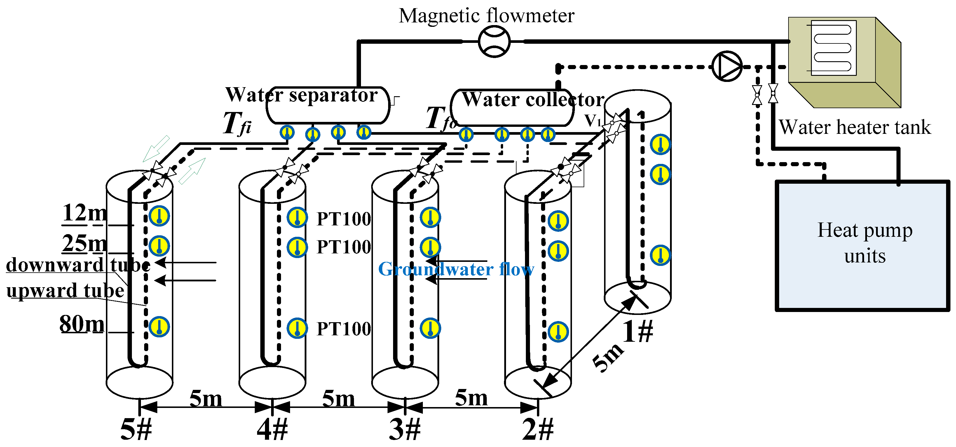
2. Experimental Investigations
3. Numerical Multilayered Model for BHE
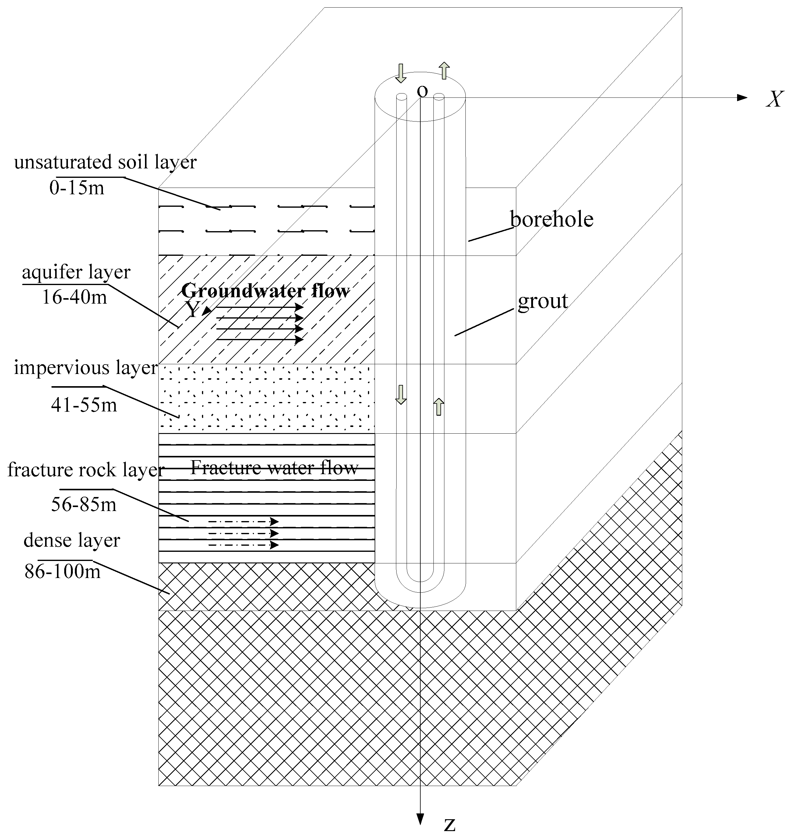
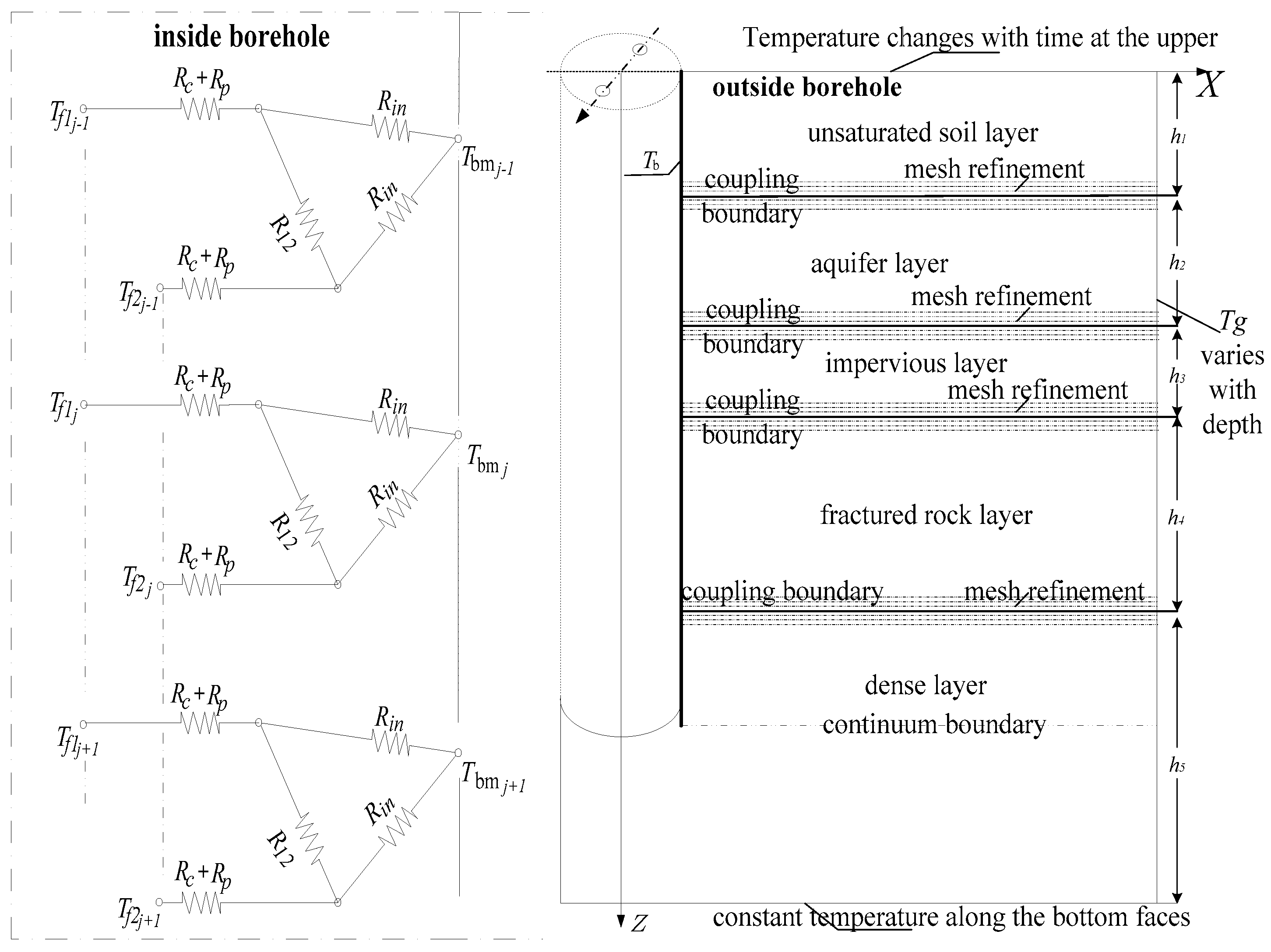
3.1. Model Description
3.2. Governing Equations
3.3. Initial and Boundary Conditions
4. Numerical Verification
4.1. Input Parameters of the Numerical Model
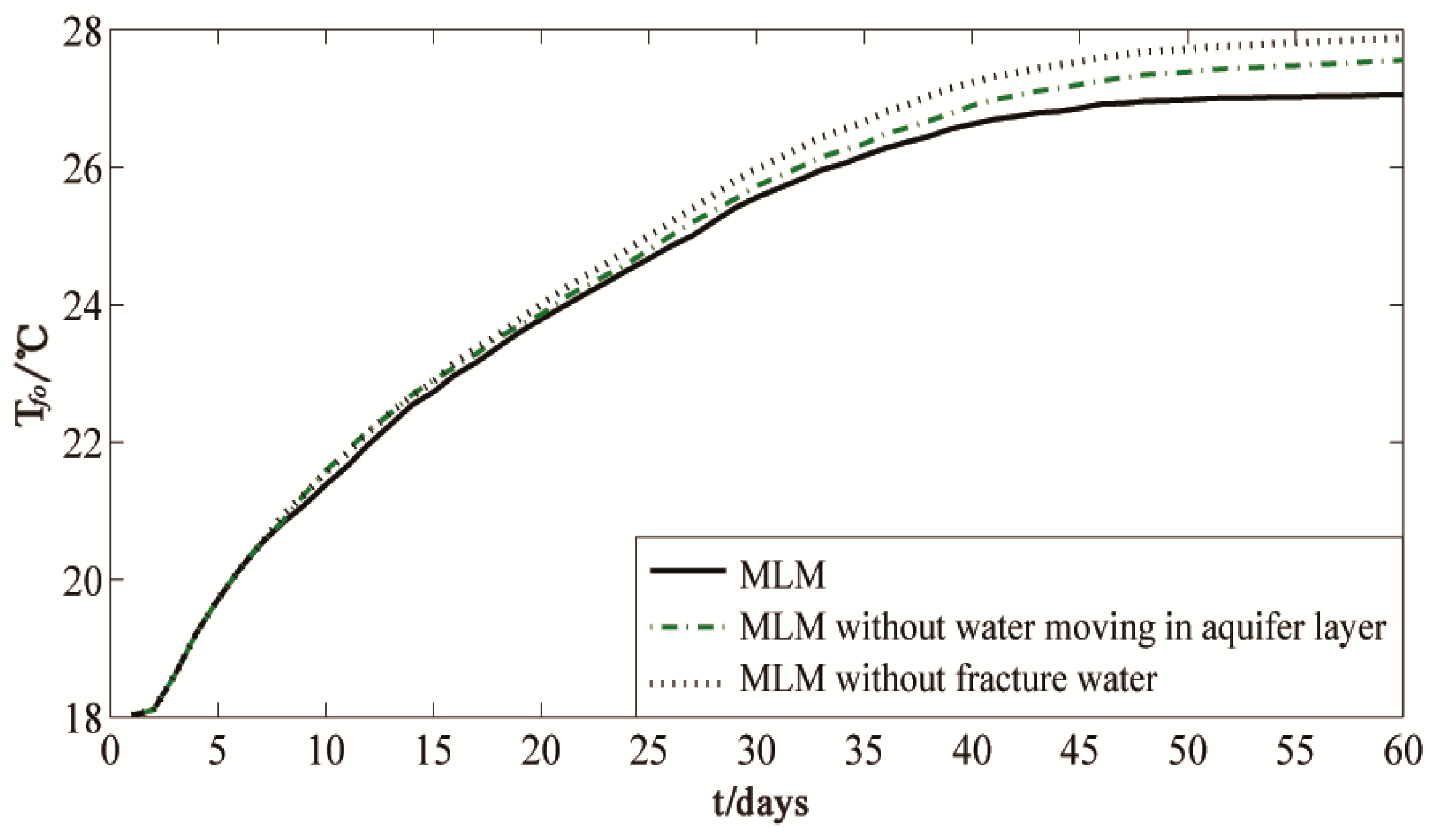
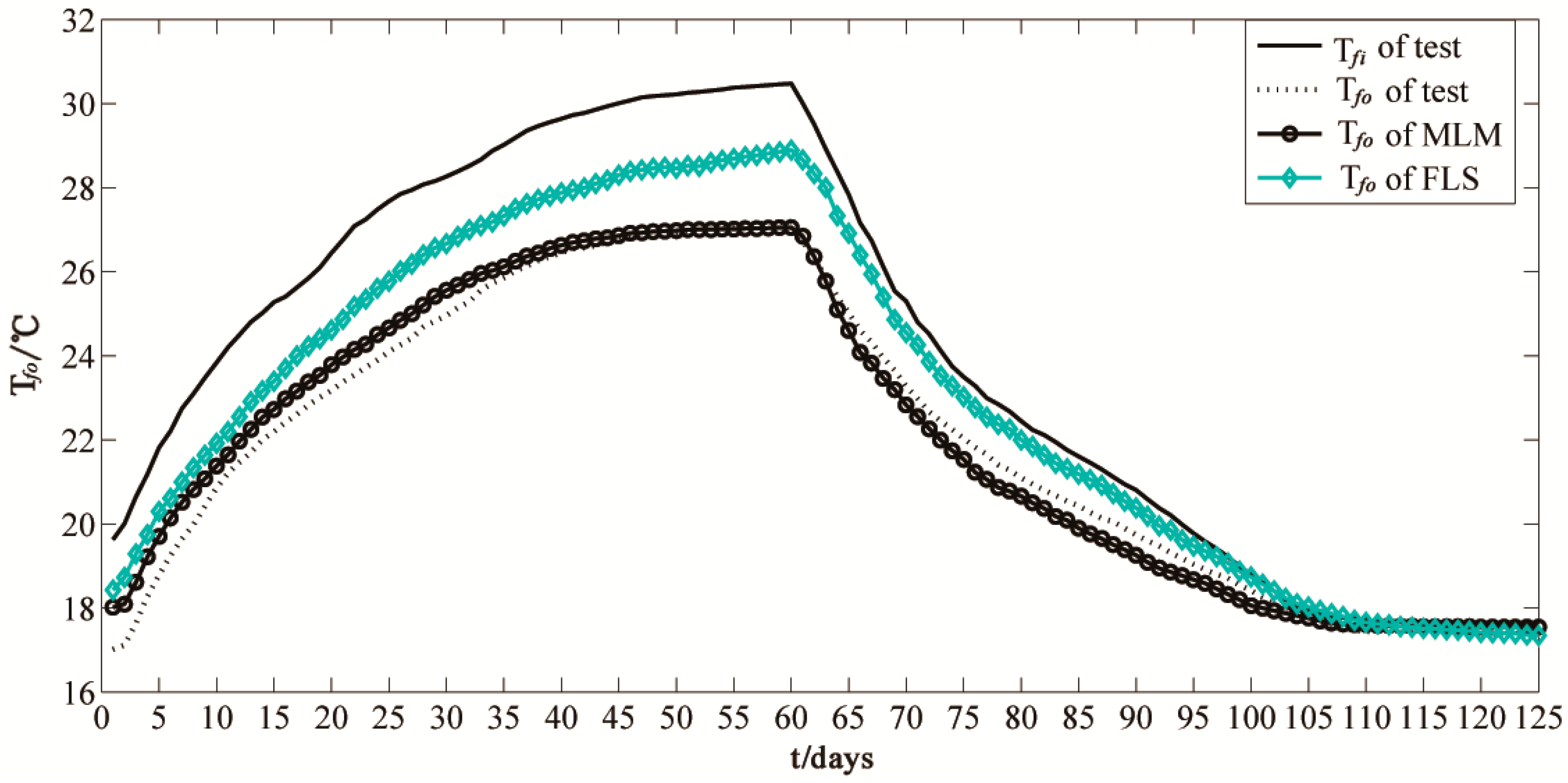
4.2. Numerical Verification
5. Results and Discussion
5.1. Comparison with FLS Model
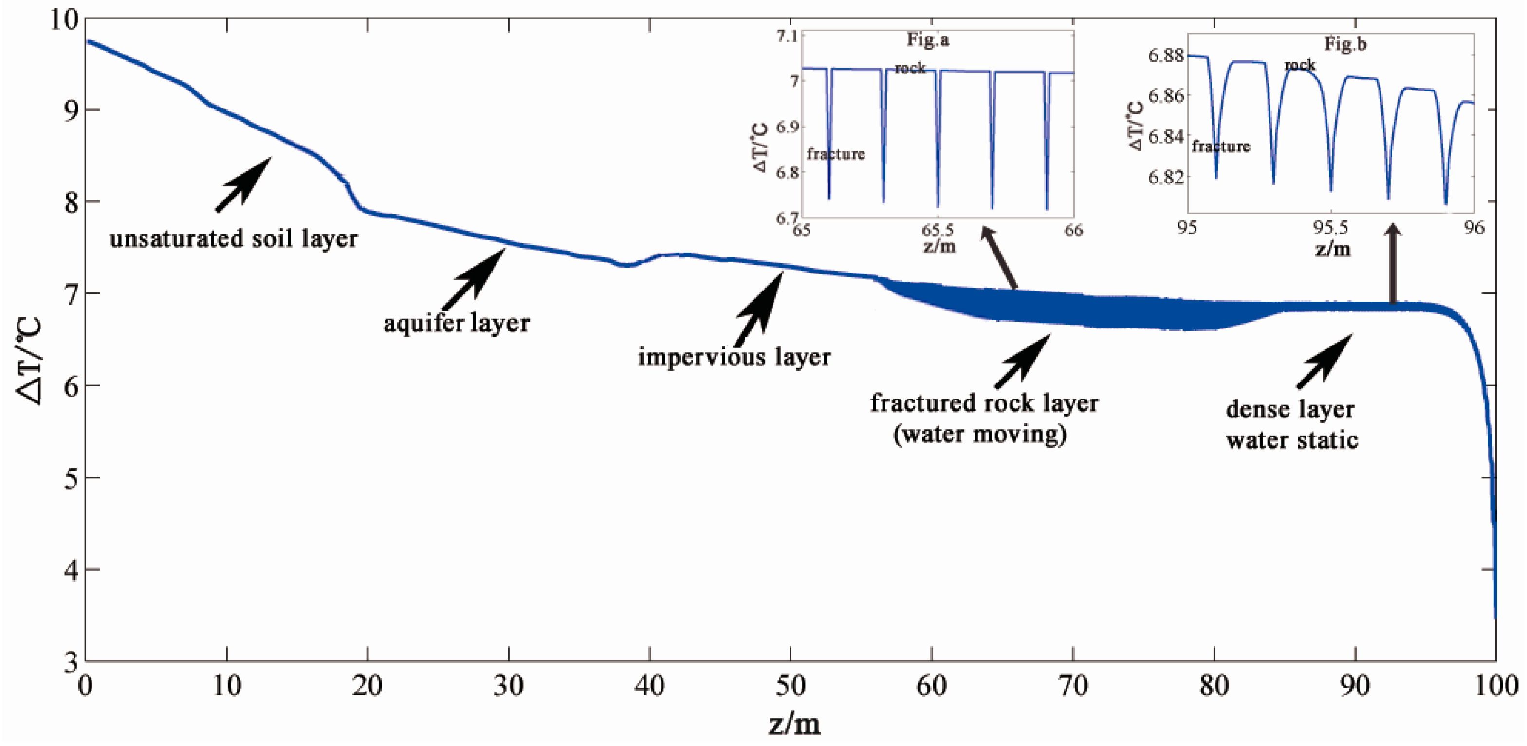
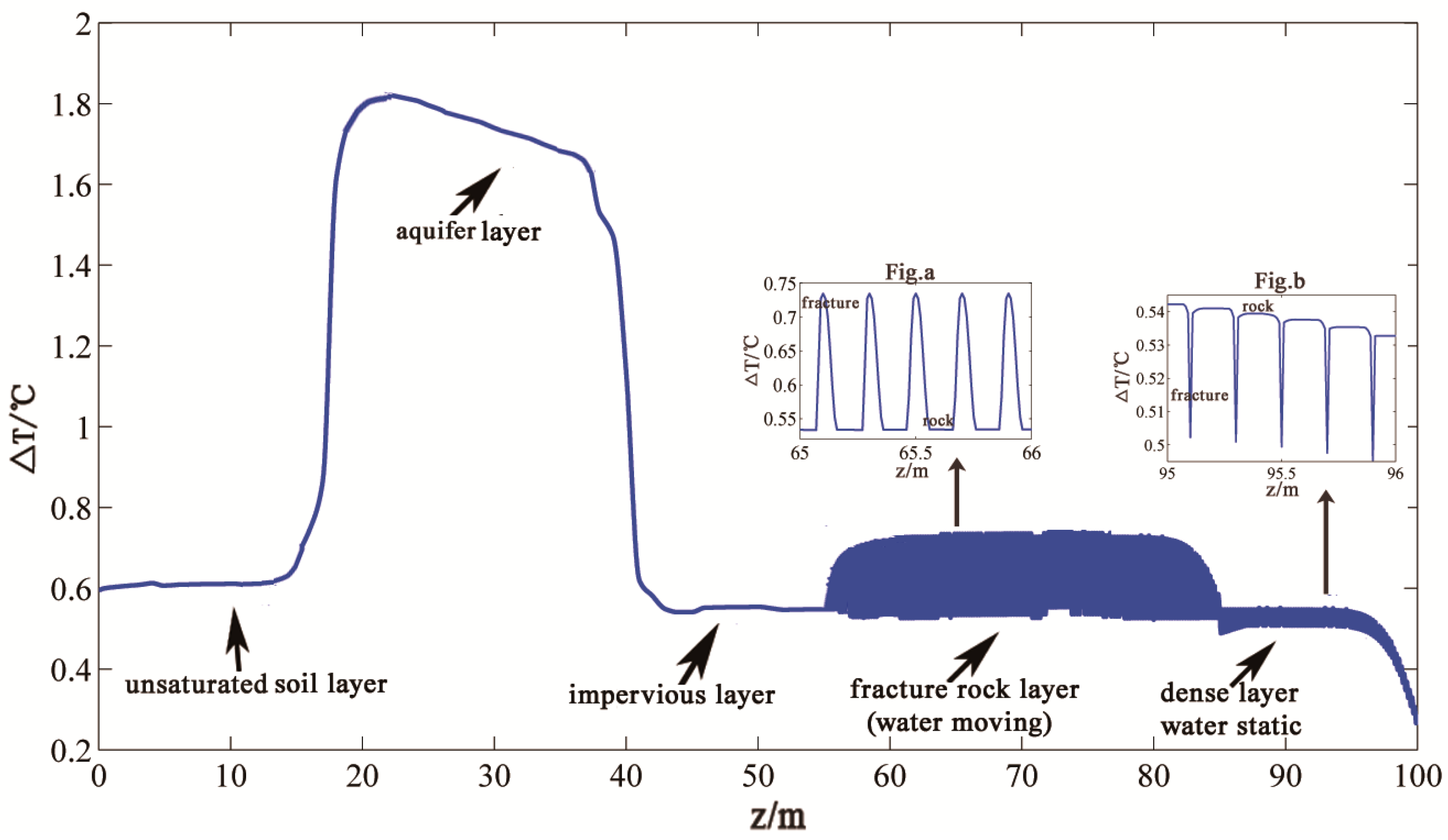
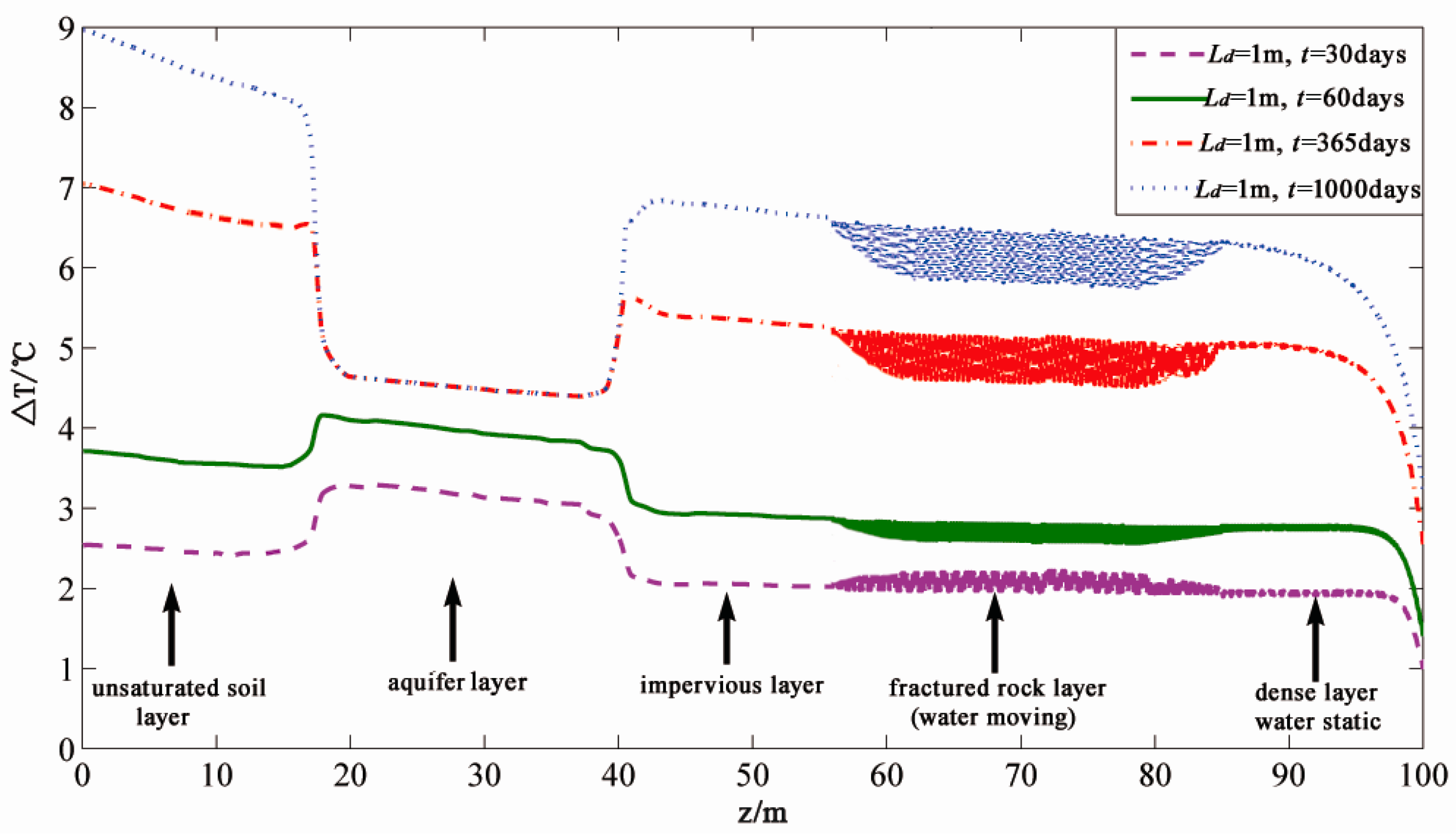
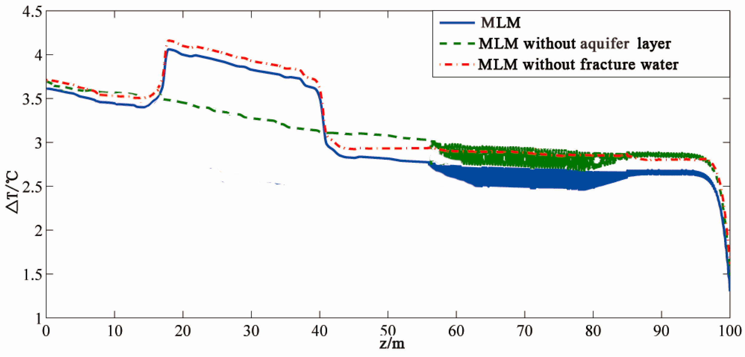
5.2. Different Multi-Layers Characteristics
6. Conclusions
Acknowledgments
Author Contributions
Conflicts of Interest
Nomenclature
| Tg | undisturbed subsurface temperature (°C) |
| Tb | borehole temperature (°C) |
| Tfi | inlet temperature of BHE (°C) |
| Tfo | outlet temperature of BHE (°C) |
| Tf1 | fluid temperature in downward tube (°C) |
| Tf2 | fluid temperature in upward tube (°C) |
| H | borehole depth (m) |
| db | borehole diameter (m) |
| dp | branch pipe diameter (m) |
| d∞ | far-field diameter (m) |
| XC | shank spacing between the center of the legs (m) |
| Af | cross-sectional area of branch pipe (m2) |
| λ | thermal conductivity (W/(m·K)) |
| a | thermal diffusivity (m2/s) |
| ρc | vol. heat capacity (J/(m3/K)) |
| φ | porosity of the medium |
| arithmetic average of the fluid temperature (°C) | |
| uf | flow velocity in tube (m/s) |
| hair | convective heat transfer coefficient between subsurface and air |
| Rfb | the borehole resistance including pipe resistance(m2 K/W) |
| R12 | thermal short-circuiting resistance between tubes (m2 K/W) |
| Rb | effective pipe-to-borehole thermal resistance (m2 K/W) |
| Re | Reynolds number |
| Subscripts | |
| s | subsurface |
| g | grout |
| j | indicate the different layer |
| f | fluid in tube |
| w | fluid in the aquifer or fracture |
| p | pipe |
| b | borehole |
| ∞ | far-field |
| Acronyms | |
| FLS | finite line source model |
| MLM | multilayered model |
References
- Nguyen, H.V.; Law, Y.L.E.; Alavy, M.; Walsh, P.R.; Leong, W.H.; Dworkin, S.B. An analysis of the factors affecting hybrid ground-source heat pump installation potential in North America. Appl. Energy 2014, 125, 28–38. [Google Scholar] [CrossRef]
- Blum, P.; Campillo, G.; Kolbel, T. Techno-economic and spatial analysis of vertical ground source heat pump systems in Germany. Energy 2011, 36, 3002–3011. [Google Scholar] [CrossRef]
- Eskilson, P.; Claesson, J. Simulation model for thermally interacting heat extraction boreholes. Number Heat Transf. 1988, 13, 149–165. [Google Scholar] [CrossRef]
- Zeng, H.Y.; Diao, N.R.; Fang, Z.H. A finite line-source model for boreholes in geothermal heat exchangers. Heat Transf. Asian Res. 2002, 31, 558–567. [Google Scholar] [CrossRef]
- Lamarche, L. A fast algorithm for the hourly simulations of ground-source heat pumps using arbitrary response factors. Renew. Energy 2009, 34, 2252–2258. [Google Scholar] [CrossRef]
- Bandos, T.V.; Montero, Á.; Fernández, E.; Santander, J.L.G.; Isidro, J.M.; Pérez, J.; de Córdoba, P.J.F.; Urchueguía, J.F. Finite line-source model for borehole heat exchangers: effect of vertical temperature variations. Geothermics 2009, 38, 263–270. [Google Scholar] [CrossRef]
- Sandler, S.; Zajaczkowski, B.; Bialko, B.; Malecha, Z.M. Evaluation of the impact of the thermal shunt effect on the U-pipe ground borehole heat exchanger performance. Geothermics 2017, 65, 244–254. [Google Scholar] [CrossRef]
- Li, M.; Li, P.; Chan, V.; Lai, A.C.K. Full-scale temperature response function (G-function) for heat transfer by borehole ground heat exchangers (GHEs) from sub-hour to decades. Appl. Energy 2014, 136, 197–205. [Google Scholar] [CrossRef]
- Li, M.; Lai, A.C.K. Analytical model for short-time responses of borehole ground heat exchangers: Model development and validation. Appl. Energy 2013, 104, 510–516. [Google Scholar] [CrossRef]
- Yang, Y.; Li, M. Short-time performance of composite-medium line-source model for predicting responses of ground heat exchangers with single U-shaped tube. Int. J. Therm. Sci. 2014, 82, 130–137. [Google Scholar] [CrossRef]
- Hu, P.; Zha, J.; Lei, F.; Zhu, N.; Wu, T. A composite cylindrical model and its application in analysis of thermal response and performance for energy pile. Energy Build. 2014, 84, 324–332. [Google Scholar] [CrossRef]
- Lei, F.; Hu, P.F.; Zhu, N.; Wu, T.H. Periodic heat flux composite model for borehole heat exchanger and its application. Appl. Energy 2015, 151, 132–142. [Google Scholar] [CrossRef]
- Carlslaw, H.S.; Jaeger, J.C. Conduction of Heat in Solids; Oxford University Press: Oxford, UK, 1959. [Google Scholar]
- Bernier, M.A.; Pinel, P.; Labib, R.; Paillot, R. A multiple load aggregation algorithm for annual hourly simulations of GCHP systems. HVAC&R Res. 2004, 10, 471–487. [Google Scholar]
- Fossa, M.; Minchio, F. The effect of borefield geometry and ground thermal load profile on hourly thermal response of geothermal heat pump systems. Energy 2013, 51, 323–329. [Google Scholar] [CrossRef]
- Colangelo, G.; Congedo, P.M.; Starace, G. Simulations of horizontal ground heat exchangers: A comparison among different configurations. Appl. Therm. Eng. 2012, 33–34, 24–32. [Google Scholar]
- Diao, N.; Li, Q.; Fang, Z. Heat transfer in ground heat exchangers with groundwater advection. Int. J. Therm. Sci. 2004, 43, 1203–1211. [Google Scholar] [CrossRef]
- Molina-Giraldo, N.; Blum, P.; Zhu, K.; Bayer, P.; Fang, Z. A moving finite line source model to simulate borehole heat exchangers with groundwater advection. Int. J. Therm. Sci. 2011, 50, 2506–25013. [Google Scholar] [CrossRef]
- Capozza, A.; De Carli, M.; Zarrella, A. Investigations on the influence of aquifers on the ground temperature in ground-source heat pump operation. Appl. Energy 2013, 107, 350–363. [Google Scholar] [CrossRef]
- Choi, J.C.; Park, J.; Lee, S.R. Numerical evaluation of the effects of groundwater flow on borehole heat exchanger arrays. Renew. Energy 2013, 52, 230–240. [Google Scholar] [CrossRef]
- Hecht-Mendez, J.; de Paly, M.; Beck, M.; Bayer, P. Optimisation of energy extraction for vertical closed-loop geothermal systems considering groundwater flow. Energy Convers. Manag. 2013, 66, 1–10. [Google Scholar] [CrossRef]
- Fujii, H.; Okubo, H.; Nishi, K.; Itoi, R.; Ohyama, K.; Shibata, K. An improved thermal response test for U-tube ground heat exchanger based on optical fiber thermometers. Geothermics 2009, 38, 399–406. [Google Scholar] [CrossRef]
- Raymond, J.; Therrien, R.; Gosselin, L.; Lefebvre, R. Numerical analysis of thermal response tests with a groundwater flow and heat transfer model. Renew. Energy 2011, 36, 315–324. [Google Scholar] [CrossRef]
- Olfman, Z.M.; Woodbury, A.D.; Bartley, J. Effects of depth and material property variations on the ground temperature response to heating by a deep vertical ground heat exchanger in purely conductive media. Geothermics 2014, 51, 9–30. [Google Scholar] [CrossRef]
- Luo, J.; Rohn, J.; Bayer, M.; Priess, A.; Xiang, W. Analysis on performance of borehole heat exchanger in a layered subsurface. Appl. Energy 2014, 123, 55–65. [Google Scholar] [CrossRef]
- Luo, J.; Rohn, J.; Xiang, W.; Bayer, M.; Priess, A.; Wilkmann, L.; Steger, H.; Zorn, R. Experimental investigation of a borehole field by enhanced geothermal response test and numerical analysis of performance of the borehole heat exchangers. Energy 2015, 84, 473–484. [Google Scholar] [CrossRef]
- Florides, G.A.; Christodoulides, P.; Pouloupatis, P. Single and double U-tube ground heat exchangers in multiple-layer substrates. Appl. Energy 2013, 102, 364–373. [Google Scholar] [CrossRef]
- Gao, Q.; Li, M.; Yu, M. Experiment and simulation of temperature characteristics of intermittently-controlled ground heat exchanges. Renew. Energy 2010, 35, 1169–1174. [Google Scholar] [CrossRef]
- Raymond, J.; Lamarche, L. Simulation of thermal response tests in a layered subsurface. Appl. Energy 2013, 109, 293–301. [Google Scholar] [CrossRef]
- Lee, C.K. Effects of multiple ground layers on thermal response test analysis and ground-source heat pump simulation. Appl. Energy 2011, 88, 4405–4410. [Google Scholar] [CrossRef]
- Doleck, A.O.; Tinjum, J.M.; Hart, D.J. Numerical modeling of ground temperature response in a ground source heat pump system (GSHP). Geotech. Spec. Publ. 2014, 234, 2755–2766. [Google Scholar]
- Lee, C.K.; Lam, H.N. A modified multi-ground-layer model for borehole ground heat exchangers with an inhomogeneous groundwater flow. Energy 2012, 47, 378–387. [Google Scholar] [CrossRef]
- Wang, Z.; Yan, A.; Guo, J. Heat transfer analysis of underground heat exchangers in multi-soil beds. Acta Energiae Sol. Sin. 2009, 30, 188–192. (In Chinese) [Google Scholar]
- Guan, C.; Zhao, W.; Hu, P. Numerical analysis on multilayer geotechnical temperature field of GSHP buried tube. J. Wuhan Inst. Technol. 2011, 33, 42–45. (In Chinese) [Google Scholar]
- Bauer, D.; Heidemann, W.; Diersch, H.J.G. Transient 3D analysis of borehole heat exchanger modeling. Geothermics 2011, 40, 250–260. [Google Scholar] [CrossRef]
- Li, Y.; Mao, J.; Geng, S.; Xu, H.; Zhang, H. Evaluation of thermal short-circuiting and influence on thermal response test for borehole heat exchanger. Geothermics 2014, 50, 136–147. [Google Scholar] [CrossRef]
- Sharqawy, M.H.; Mokheimer, E.M.; Badr, H.M. Effective pipe-to-borehole thermal resistance for vertical ground heat exchangers. Geothermics 2009, 38, 271–277. [Google Scholar] [CrossRef]
- Gehlin, S.E.A.; Hellstrom, G. Influence on thermal response test by groundwater flow in vertical fractures in hard rock. Renew. Energy 2003, 28, 2221–2238. [Google Scholar] [CrossRef]
- Cheng, A.H.D.; Ghassemi, A.; Detoumay, E. Integral equation solution of heat extraction from a fracture in hot dry rock. Int. J. Numer. Anal. Methods Geomech. 2001, 25, 1327–1338. [Google Scholar] [CrossRef]
- Chiasson, A.; O’Connell, A. New analytical solution for sizing vertical borehole ground heat exchangers in environments with significant groundwater flow: parameter estimation from thermal response test data. HVAC R Res. 2011, 17, 1000–1011. [Google Scholar]
- Koohi-Fayegh, S.; Rosen, M.A. An analytical approach to evaluating the effect of thermal interaction of geothermal heat exchangers on ground heat pump efficiency. Energy Convers. Manag. 2014, 78, 184–192. [Google Scholar] [CrossRef]


| Depth (m) | Lithology |
|---|---|
| 0–15 m | unsaturated soil |
| 16–40 m | aquifer layer |
| 41–55 m | impervious layer |
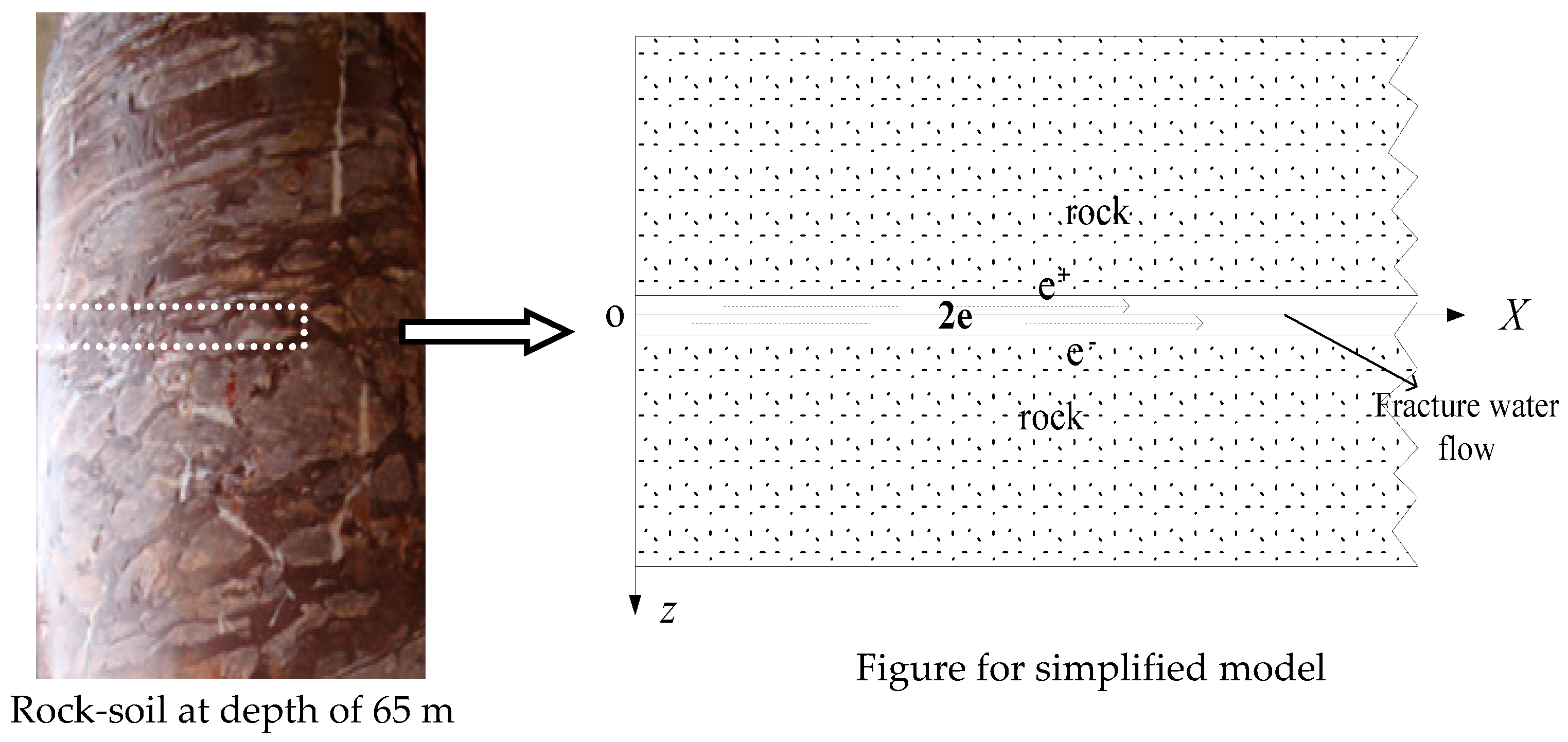
| 56–85 m | fractured rock (water moving) |
| 86–100 m | dense layer (water static) |
| Depth z [m] | Thermal Conductivity λs [W/m·K] | vol. heat Capacity Cs [J/m3/K] | Depth z [m] | Thermal Conductivity λs [W/m·K] | Vol. Heat Capacity Cs [J/m3/k] |
|---|---|---|---|---|---|
| 3 | 1.51 | 1,963,000 | 30 | 1.82 | 2,038,400 |
| 4 | 1.53 | 1,957,500 | 35 | 1.80 | 2,100,000 |
| 8 | 1.62 | 2,079,000 | 38 | 1.84 | 2,300,000 |
| 10 | 1.65 | 2,010,000 | 42 | 2.0 | 2406,400 |
| 13 | 1.66 | 1,982,400 | 50 | 2.1 | 2,361,800 |
| 16 | 1.68 | 1,960,200 | 56 | 2.2 | 2,430,400 |
| 18 | 1.70 | 2,016,000 | 72 | 2.2 | 2,400,000 |
| 22 | 1.72 | 1,928,500 | 80 | 2.2 | 2,548,000 |
| 25 | 1.72 | 1,919,000 | 88 | 2.21 | 2,510,000 |
| 28 | 1.84 | 2,005,600 | 96 | 2.18 | 2,410,000 |
| Parameter | Unit | Value |
|---|---|---|
| borehole diameter (db) | (m) | 0.12 |
| pipe diameter (dp) | (m) | 0.032 |
| pipe thickness (δ) | (m) | 0.0025 |
| shank spacing (XC) | (m) | 0.064 |
| grout thermal conductivity (λg) | (W/m·K) | 2.4 |
| grout vol. heat capacity (ρgcg) | (J/m3/K) | 3.2 × 10⁶ |
| pipe thermal conductivity (λp) | (W/m·K) | 0.6 |
| borehole depth (H) | (m) | 100 |
| flow velocity in tube (uf) | (m/s) | 0.72 |
© 2017 by the authors. Licensee MDPI, Basel, Switzerland. This article is an open access article distributed under the terms and conditions of the Creative Commons Attribution (CC BY) license ( http://creativecommons.org/licenses/by/4.0/).
Share and Cite
Li, Y.; Geng, S.; Han, X.; Zhang, H.; Peng, F. Performance Evaluation of Borehole Heat Exchanger in Multilayered Subsurface. Sustainability 2017, 9, 356. https://doi.org/10.3390/su9030356
Li Y, Geng S, Han X, Zhang H, Peng F. Performance Evaluation of Borehole Heat Exchanger in Multilayered Subsurface. Sustainability. 2017; 9(3):356. https://doi.org/10.3390/su9030356
Chicago/Turabian StyleLi, Yong, Shibin Geng, Xu Han, Hua Zhang, and Fusheng Peng. 2017. "Performance Evaluation of Borehole Heat Exchanger in Multilayered Subsurface" Sustainability 9, no. 3: 356. https://doi.org/10.3390/su9030356