Environmentally Friendly Supplier Selection Using Prospect Theory

Abstract

This paper proposes an optimal selection method to address the real-world problem of environmentally friendly supplier selection, based on prospect theory. This study adopted the manufacturer’s point of view, and considered the manufacturer’s psychological and behavioral factors in the process of choosing suppliers. The first step was to build supplier-selection indexes for manufacturers. Then, the study assessed the attribute of manufacturer expectations as a reference point. Next, index gains and losses were evaluated against the expectation reference point, yielding a payoff matrix and loss matrix. Finally, the study used prospect theory to calculate the comprehensive prospect value of each supplier; comprehensive prospect values were sorted in descending order to help manufacturers make the best choice.

1. Introduction

In the 1970s, T.L. Satty studied the problem of supplier evaluation and selection, proposing that supplier selection be based on analytic hierarchy process (AHP). This qualitative analysis involved a pairwise comparison of different evaluation factors, resulting in a judgment matrix. Second, a feature vector corresponding to the largest eigenvalue as a coefficient was used to evaluate each plan’s weight. This enabled supplier evaluation and selection.

Degraeve et al. [1] studied the total cost of partner selection, proposing a cost analysis method based on activity (ABC analysis). This method analyzes the direct and indirect costs of enterprises based on procurement size; supplier selection is made by calculating the supplier’s total cost. Arikan [2] used a multi-objective linear programming model to select the supplier. Ghodsypour et al. [3] selected suppliers using the method of combined AHP linear programming. Shiromaru et al. [4] used a selection based on fuzzy theory to select suppliers. Huang et al. [5] proposed a random data envelopment analysis (DEA) method with AHP to select suppliers; by introducing random variables, they addressed the shortcomings of weight selection in the DEA method. This method converted the subjective judgment of the supplier selection process into a credibility judgment, improving the reliability of supplier evaluation.

Xu et al. [6] introduced the grey clustering decision-making method into the supplier selection process. This allowed the quantitative appraisal of the clustering object and cluster index. Suppliers are then ranked, providing a supplier selection reference for manufacturers. Zhang et al. [7] selected suppliers using AHP to determine the weight and to quantify qualitative problems; neural logic network was used to simulate logical reasoning, resulting in a supplier selection model. The model assigned different weights based on expert input for different field indices. This optimized the pure AHP research method, and used AHP to determine the weights of logical network levels, making the network structure more scientific and applicable.

In researching supplier selection methods, Wang et al. [8] proposed a supplier selection method that combined AHP, a preference order structure evaluation method, and an interaction method. They determined the structure of the supply selection problem and the evaluation criteria weights using AHP; evaluated the candidate suppliers in order of their preference structure method; and analyzed sensitivity using an interactive aided geometric analysis method. This resulted in a candidate supplier ranking.

Some scholars have used fuzzy mathematics methods to study the problem of project selection. Ruan et al. [9,10] studied the monitoring and evaluation of the freshness of fruits using an interval number method. They also optimized a medical supply multimodal transport problem using a balanced fuzzy clustering method, and optimized the allocation of disaster relief materials using interval and fuzzy number methods. Ruan et al. [11,12] summarized the application of cloud-computing algorithms over the past ten years. This provided new insights for subsequent scholars using cloud-computing algorithms to study the supplier selection problem. Zeydan et al. [13] used NGT (Nominal Group Technique) and fuzzy network analysis (Fuzzy ANP, FANP) to calculate the importance of determining the index, resulting in a supplier selection model. Kannan et al. [14] used the TOPSIS (Technique for Order Preference by Similarity to Ideal Solution) method, geometric mean, and cascading average fuzzy ideal solution. This allowed them to rank alternative green suppliers in order of importance, and to test differences in project scheduling caused by using different methods associated with the Spearman rank correlation coefficient.

In their studies on optimal supplier determination, Sanayei et al. [15] converted the linguistic variables characterizing evaluation value and weight information with a triangular fuzzy number and trapezoid fuzzy number; they then used the fuzzy VIKOR method to establish an optimal supplier model. Shemshadi et al. [16] transformed the trapezoidal fuzzy number to an exact number, using the Shannon entropy weighting method combined with the improved VIKOR method. This created a new way to sort and select the most satisfactory supplier from many alternatives. Sahu et al. [17] converted evaluation information and attribute weights provided about green suppliers using the trapezoidal fuzzy number method, and selected the best supplier using the resulting scheme. Chung et al. [18] established a green supplier selection and guidance mechanism by integrating the features of an ANP (Analytic Network Process) and an IPA (Importance-Performance Analysis). This approach supports sustainable management for green supply chains.

In studying a logistics supplier selection decision model, Boran et al. [19] considered both expert preference and a related evaluation index. Considering the arbitrary selection of an evaluation standard by an expert group evaluating service providers, they evaluated data consistency using a transformation function of different evaluation scales. This yielded a group decision to select a logistics supplier using a maximum entropy configuration model and Choquet integral. Junior et al. [20] researched the selection of logistic suppliers by determining the weights of second level indexes using the TOPSIS method. They also adopted a qualitative AHP to determine the weights of the first- level indicators. This resulted in a fuzzy comprehensive evaluation model based on combining the TOPSIS method and AHP method. The result was an automobile reverse logistics supplier evaluation index system. Wu et al. [21] and Liu et al. [22] applied this same concept and fuzzy comprehensive evaluation method to model supplier selection. Once the qualitative factors and fuzzy factors were quantified, the fuzzy comprehensive supplier selection evaluation model was established. Kuo et al. [23] proposed a novel hybrid multiple-criteria decision-making (MCDM) method to evaluate green suppliers in an electronics company. The Decision-Making Trial and Evaluation Laboratory (DEMATEL) applied the Analytic Network Process (ANP) method (known as DANP) to determine both the importance of evaluation criteria in selecting suppliers and the causal relationships between them. Finally, the VIKOR method was used to evaluate the environmental performance of suppliers and to obtain a solution for each evaluation criterion.

In studying the supplier selection problem, scholars have also conducted qualitative and quantitative research based on expected utility theory. Research using this method is confined to the definite object and methods for using the associated certainty; there have been many research achievements in this area. However, in real life, supply chain systems are complex and changeable organisms [24]. There are also many risks associated with factors such as policy, environment, management, information asymmetry, and others. Research has revealed differences in information uncertainty; related studies using fuzzy mathematics, grey systems, and rough set methods have also been applied to the supplier selection problem. These studies have achieved good theoretical and practical results. The deterministic method associated with a specific object of study results in a deterministic numerical index to select suppliers in uncertain situations. The evaluation index developed using a fuzzy interval or numerical language form is more consistent with the fuzzy research paradigm. Further, the research conclusions are more representative and practical, as decision makers making actual decisions need a framework of limited rationality to select the most satisfactory solution [25,26,27,28].

Based on this, this paper proposes a new method to optimize decision analysis based on prospect theory, focusing on the problem of multiple-attribute decision making. This method has been used successfully in economics and finance. The theory has four key features that distinguish prospect theory from mean variance theory, which is the traditional approach to modelling decision making. First, traditional theory proposes that people choose among alternatives based on how the outcomes will affect their overall outlook. However, prospect theory proposes instead that people evaluate outcomes in terms of gains and losses relative to a reference point. Second, mean variance analysis assumes that people are risk averse in all their choices. In contrast, with prospect theory, agents are assumed to be risk averse with respect to gains, but seek risk when all changes in income are framed as losses. The third feature of prospect theory is “loss aversion.” Fourth, in utility theory, risk is treated objectively based on its probabilities. In contrast, the utility under prospect theory does not depend on the original probability, but rather on the transformed probability, also known as decision weights.

The rest of this paper is organized as follows. The first part of this study establishes a supplier selection evaluation index system. Next, parameter descriptions are constructed, yielding a decision model based on prospect theory. The third part of the paper considers the practical example of integrated circuit manufacturers that are selecting electronic component suppliers. The model is then applied and the results analyzed and compared, demonstrating the method’s effectiveness.

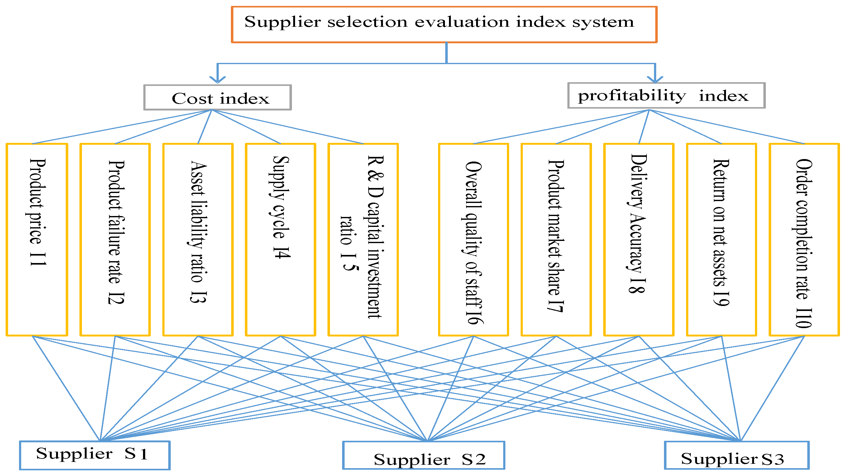
2. Supplier Selection Decision Model

Selecting criteria is a fundamental step in constructing a decision-making model, especially in supply chain selection. Companies should select suppliers based on the criteria that are effective and relative to the company’s activity, and that also conform to the environmental factors around them. Commonly used criteria include quality, delivery, cost/price, manufacturing capability, service, management, technology, research, flexibility, finance, reputation, relationship, risk and safety, and the environment [29]. Selecting a supplier evaluation index based on the prospect theory requires us to comprehensively capture the suppliers’ internal factors and related conditions. We must also consider the psychological behavior of manufacturers in making selections, and follow minimum risk and flexible operational principles. This means that the selected indicators must respond to the supplier’s ability to deal with risk, and also align with the manufacturer’s specific circumstances [27]. This results in appropriate changes and increases or decreases to the index system [28,29,30]. Therefore, based on the existing academic research, to start manufacturer optimization of supplier selection, we select ten evaluation indexes close to the manufacturer’s actual choices of reference indicators [30,31,32,33,34,35]. Figure 1 depicts the ten indicators of the hierarchical model based on profitability index and cost index. They include:

• Cost index:

  1.1.

  Product price (I1): the cost directly related to obtaining the corresponding supplier’s product.

  1.2.

  Product failure ratio (I2): the product’s failure rate when environmentally friendly factors are considered. For the environmentally friendly supplier selection problem, the environmental performance index (EPI) is one method to quantify and numerically mark a supplier’s environmental performance. If a product has environmentally friendly attributes, it can be accepted as a satisfactory product; this directly connects the product failure ratio to an index related to the environment.

  1.3.

  Asset liability ratio (I3): the proportion of a company’s assets that are being financed with debt, rather than equity. This ratio is used to determine the financial risk of a business.

  1.4.

  Supply cycle (I4): the speed at which the supplier provides the ordered products.

  1.5.

  Research and development (R & D) capital investment ratio (I5): the ratio of R & D investment divided by the revenues.

• Profitability index:

  2.1.

  The Quality of the Staff (I6): staff quality indicates employee quality.

  2.2.

  Product market share (I7): percentage of a market (defined in terms of either units or revenue) accounted for by a specific entity.

  2.3.

  Delivery accuracy (I8): an important operational performance measure that combines non-financial elements, namely time and quality.

  2.4.

  Return on net assets (I9): a measure of financial performance, calculated as net income divided by fixed assets and net working capital.

  2.5.

  Order Completion Rate (I10): percent of orders shipped containing all items of a sales order. It is calculated as the number of annual sales orders delivered as a complete shipment according to the sales order (with no items on back order), divided by the total number of annual sales orders.

This paper proposes a multi-attribute decision-making method based on prospect theory. Manufacturers are described using an indicator system, with established expectations as a reference point. Relative to this reference point, gains and losses are calculated based on different supplier value indicators. This establishes a risk return and risk loss matrix. Using prospect theory, the study establishes a prospective decision matrix. Based on this, it is possible to sort through comprehensive values associated with the prospect of selecting each supplier. This leads to the optimal manufacturer selection, providing a reference. The following discussion provides the income and loss calculation methods, the future value of the calculation, and the supplier ranking method.

Table 1. Variable definition.

Variable	Meaning
$S=\{S_1,S_2,\mathrm{...},S_i,\mathrm{...},S_m\}$	A collection of m supplier alternatives
$m$	Number of suppliers
$I=\{I_1,I_2,\mathrm{...},I_i,\mathrm{...},I_n\}$	A set of n indicators
$N=\{1,2,\mathrm{...},n\}$	Subscripted collections of index
$N_1,N_2 \mathrm{and} N_1\cup N_2=N,N_1\cap N_2=\varnothing$	Subscripted collections of profit index and cost index
$w=(w_1,w_2,\mathrm{...},w_n),w_j\ge 0 \mathrm{and} {\displaystyle \sum _{j=1}^n{w}_j=1}$	Weight vector of index
Y	The index of natural state
$A=\{A_1,A_2,\mathrm{...},A_t,\mathrm{...},A_y\}$	Natural state set
$Y=\left\{1,2,\cdots ,y\right\}$	A collection of natural states of y
$p_t,p_t\ge 0 and {\displaystyle \sum _{t=1}^y{p}_t=1}$	Probability of occurrence of state $A_t$
$E=(e_1,e_2,\mathrm{...},e_n)$	The desired vector of the index
$e_j=(e_j^1,e_j^2,\mathrm{...},e_j^y)$	The expectation of decision makers for attribute $I_j$
$e_j^t$	The status of $A_t$ decision makers to target the expectations of $I_j$
$X={\left[x_{ij}^t\right]}_{m\times n}$	Risk decision matrix
$x_{ij}^t$	The status of $A_t$, supplier $S_i$ aims at decision results of $I_j$
$x_{ij}^{t1}$,$x_{ij}^{tz}$	Lower and upper bounds of interval numbers
$a_{ij}^t,b_{ij}^t,c_{ij}^t,d_{ij}^t,a_{ij1}^t,b_{ij}^t,c_{ij}^t,d_{ij1}^t$	Value of fuzzy number
$I^K=\{I_1,I_2,\mathrm{...},I_{J_1}\}$	Index value is the index set of clear number
$I^L=\{I_{J_1+1},I_{J_1+2},\mathrm{...},I_{J_2}\}$	Index value is the index set of interval number
$I^F=\{I_{J_2+1},I_{J_2+2},\mathrm{...},I_n\}$	Index value is the index set of intuitionistic trapezoidal fuzzy number
$N^K=\{1,2,\mathrm{...},J_1\}$	Subscripted collections of index subset $I^K$
$N^L=\{J_1+1,J_1+2,\mathrm{...},J_2\}$	Subscripted collections of index subset $I^L$
$N^F=\{J_2+1,J_2+2,\mathrm{...},n\}$	Subscripted collections of index subset $I^F$

defines each variable.

Assume that expectation $e_j^t$ is a clear number; the type of index value $x_{ij}^t$ has three forms: clear number, interval number, and trapezoid fuzzy numbers. The three types of index values are described as follows.

(1) When the index $I_j\in I^K$, let $x_{ij}^t={x^{\prime }}_{ij}^t$, ${x^{\prime }}_{ij}^t$ is a real number type, $i\in M,j\in N^K,T\in Y$.

(2) When the index $I_j\in I^I$, let $x_{ij}^t={\overline{x}}_{ij}^t$, is the number of intervals, that is ${\overline{x}}_{ij}^t=[x_{ij}^{t1},x_{ij}^{tz}]$, $x_{ij}^{t1}<x_{ij}^{tz},i\in M,j\in N^L,T\in Y$ is satisfied.

Because the number of intervals is derived from random sampling calculations, it can be assumed that interval $[x_{ij}^{t1},x_{ij}^{tz}]$ is relatively immobile. The actual value of the index $x$ in the $[x_{ij}^{t1},x_{ij}^{tz}]$ interval is the random value, and is subject to a distribution. Zhang et al. note that the normal distribution and uniform distribution are the most commonly used distributions, so they are applied with the two cases [32]. If every interval is a random interval through the sampling calculations, however, the comprehensive evaluation value of the decision scheme is an objective value. This ensures that the objective value is included in the corresponding interval. At the same time, each point in the interval has the same probability of covering the comprehensive evaluation value. As such, we can assume the relative interval is relatively fixed; the comprehensive evaluation value is the random value; and the evaluation value obeys a uniform distribution. When the probability density function is the uniform distribution, the probability density function is:

$$f_{ij}^t(x)=\{\begin{array}{c}\frac{1}{x_{ij}^{tz}-x_{ij}^{t1}},x_{ij}^{t1}\le x\le x_{ij}^{tz}\\ 0,other\end{array}，i\in M,j\in N^I,t\in Y\begin{array}{}\end{array}$$

(1)

If every interval is a random interval through the sampling calculations, such as intervals $\tilde{a}=\left[a^L,a^U\right]$ and $\tilde{b}=\left[b^L,b^U\right]$, the intervals are random because of the random sampling, and there are cross-sections for the two interval numbers. The scheme’s evaluation value has the probability of 99.73% in interval $\tilde{c}=\left[\min (a^L,b^L),\max (a^U,b^U)\right]$ (Following the 3$\sigma$ principle). The evaluation value is covered by the random point, which can be considered as the “interval.” The evaluation value is randomly placed in a certain position of the “interval,” and obeys the normal distribution of $N({\mu }_c,{\sigma }_c^2)$, ${\mu }_c=(\min (a^L,b^L)+\max (a^U,b^U))/2$, ${\sigma }_c=(\max (a^U,b^U)-\min (a^L,b^L))/6$.

When $x$ follows the normal distribution of $N({\mu }_{ij}^t,{({\sigma }_{ij}^t)}^2)$, the probability of $x$ is 99.73%, covered by the internal $[x_{ij}^{t1},x_{ij}^{tz}]$, ${\mu }_{ij}^t=\frac{x_{ij}^{t1}+x_{ij}^{tz}}{2},{\sigma }_{ij}^t=\frac{(\left|x_{ij}^{t1}-x_{ij}^{tz}\right|)}{6}$. The probability is:

$$f_{ij}^t(x)=\frac{1}{\sqrt{2\pi }{\sigma }_{ij}^t}{e}^{\frac{{(x-{\mu }_{ij}^t)}^2}{2{({\sigma }_{ij}^t)}^2}},i\in M,j\in N^I,t\in Y\begin{array}{}\end{array}$$

(2)

(3) When the index is $I_j\in I^F$, let $x_{ij}^t={\tilde{x}}_{ij}^t$, and ${\tilde{x}}_{ij}^t$ is the intuitionistic trapezoidal fuzzy number. That is:

$${\tilde{x}}_{ij}^t=\langle \left(\left[a_{ij}^t,b_{ij}^t,c_{ij}^t,d_{ij}^t\right];{\phi }_x\right),\left(\left[a_{ij1}^t,b_{ij}^t,c_{ij}^t,d_{ij1}^t\right];{\tau }_x\right)\rangle ,$$

$$0\le {\phi }_x\le 1,0\le {\tau }_x\le 1,{\phi }_x+{\tau }_x\le 1,$$

$$a_{ij}^t,b_{ij}^t,c_{ij}^t,d_{ij}^t,a_{ij1}^t,d_{ij1}^t\in R,$$

Its membership is:

$${\phi }_{ij}^t(x)=\{\begin{array}{c}\frac{x-a_{ij}^t}{b_{ij}^t-a_{ij}^t},a_{ij}^t\le x\le b_{ij}^t\\ {\phi }_{ij}^t,b_{ij}^t\le x\le c_{ij}^t\\ \frac{d_{ij}^t-x}{d_{ij}^t-c_{ij}^t},c_{ij}^t\le x\le d_{ij}^t\\ 0,other\end{array}，i\in M,j\in N^F,t\in Y\begin{array}{}\end{array}$$

(3)

In general, in the intuitionistic trapezoidal fuzzy number ${\tilde{x}}_{ij}^t$, there is $\left[a_{ij}^t,b_{ij}^t,c_{ij}^t,d_{ij}^t\right]=\left[a_{ij1}^t,b_{ij}^t,c_{ij}^t,d_{ij1}^t\right]$, recorded as ${\tilde{x}}_{ij}^t=\left(\left[a_{ij}^t,b_{ij}^t,c_{ij}^t,d_{ij}^t\right];{\varphi }_x,{\tau }_{ij}^t\right)$. This study evaluates the fuzzy number of this type. The ${\delta }_{ij}^t(x)=1-{\phi }_{ij}^t-{\tau }_{ij}^t$ indicates the degree of hesitation: the smaller the value, the more definitive the fuzzy number.

2.1. Calculation of Gain and Loss

The first step in calculating gain and loss is to determine the reference point of each index. The expectations given by the manufacturer are accepted as the reference point; as such, this study used the manufacturer’s expectation of $e_j=(e_j^1,e_j^2,\cdots ,e_j^y)$ as the reference point of each index.

The next step was to calculate the profit and loss of each supplier index value relative to the reference point.

(1) When the index is $I_j\in I^K$, there are two possible relationships between the index value ${x^{\prime }}_{ij}^t$ and the reference point $e_j^t$. ${x^{\prime }}_{ij}^t<e_j^t$ and ${x^{\prime }}_{ij}^t\ge e_j^t$. The following two situations inform the income and loss calculation formula.

(a) When ${x^{\prime }}_{ij}^t<e_j^t$, the formula for calculating the value of the profit $G_{ij}^t$ of the index value ${x^{\prime }}_{ij}^t$ relative to the reference point $e_j^t$ is:

$$G_{ij}^t=\{\begin{array}{ll}0，& i\in M,j\in N^K\cap N^1,t\in Y\\ e_{ij}^t-{x^{\prime }}_{ij}^t,& i\in M,j\in N^K\cap N^2,t\in Y\end{array}\begin{array}{}\end{array}$$

(4)

The formula for calculating the loss of $L_{ij}^t$ is:

$$L_{ij}^t=\{\begin{array}{c}{x^{\prime }}_{ij}^t-e_{ij}^t，i\in M,j\in N^K\cap N^1,t\in Y\\ 0,i\in M,j\in N^K\cap N^2,t\in Y\end{array}\begin{array}{}\end{array}$$

(5)

(b) When ${x^{\prime }}_{ij}^t\ge e_j^t$, the formula for calculating the value of the profit $G_{ij}^t$ of the index value ${x^{\prime }}_{ij}^t$ relative to the reference point $e_j^t$ is:

$$G_{ij}^t=\{\begin{array}{c}{x^{\prime }}_{ij}^t-e_{ij}^t，i\in M,j\in N^K\cap N^1,t\in Y\\ 0,i\in M,j\in N^K\cap N^2,t\in Y\end{array}\begin{array}{}\end{array}$$

(6)

The formula for calculating the loss of $L_{ij}^t$ is:

$$L_{ij}^t=\{\begin{array}{ll}0，& i\in M,j\in N^K\cap N^1,t\in Y\\ e_{ij}^t-{x^{\prime }}_{ij}^t,& i\in M,j\in N^K\cap N^2,t\in Y\end{array}\begin{array}{}\end{array}$$

(7)

(2) When the index is $I_j\in I^I$, in the three considered cases, the relationship between the index value ${\overline{x}}_{ij}^t$ and the reference point $e_j^t$ is: $x_{ij}^{tz}\le e_j^t$, $x_{ij}^{t1}\le {\overline{x}}_{ij}^t\le x_{ij}^{tz}$ and $x_{ij}^{t1}\ge e_j^t$. In this case, the calculation formula for the gain and loss are, respectively:

(a) When $x_{ij}^{tz}\le e_j^t$, ${\overline{x}}_{ij}^t\prec e_j^t$, the profit $G_{ij}^t$ of the index value ${x^{\prime }}_{ij}^t$ relative to the reference point $e_j^t$ is:

$$G_{ij}^t=\{\begin{array}{c}0，\begin{array}{}\end{array}i\in M,j\in N^K\cap N^1,t\in Y\\ {\displaystyle {\int }_{x_{ij}^{t1}}^{x_{ij}^{tz}}(e_j^t-x)f_{ij}^t(x)dx},i\in M,j\in N^K\cap N^2,t\in Y\end{array}\begin{array}{}\end{array}$$

(8)

Loss $L_{ij}^t$ is:

$$L_{ij}^t=\{\begin{array}{c}{\displaystyle {\int }_{x_{ij}^{t1}}^{x_{ij}^{tz}}(x-e_j^t)f_{ij}^t(x)dx}，i\in M,j\in N^K\cap N^1,t\in Y\\ 0,\begin{array}{}\end{array}i\in M,j\in N^K\cap N^2,t\in Y\end{array}\begin{array}{}\end{array}$$

(9)

(b) When $x_{ij}^{t1}\le {\overline{x}}_{ij}^t\le x_{ij}^{tz}$, $e_j^t$ will be divided into two sub-ranges, recorded as ${\overline{x}}_{ij}^{t*}=[x_{ij}^{t1},e_j^t]$ and ${\overline{x}}_{ij}^{t**}=[e_j^t,x_{ij}^{t\mathrm{z}}]$, then ${\overline{x}}_{ij}^{t*}\prec e_j^t$ and ${\overline{x}}_{ij}^{t**}\succ e_j^t$. Therefore, the profit $G_{ij}^t$ of the index value ${x^{\prime }}_{ij}^t$ relative to the reference point $e_j^t$ is:

$$G_{ij}^t=\{\begin{array}{c}{\displaystyle {\int }_{e_j^t}^{x_{ij}^{tz}}(x-e_j^t)f_{ij}^t(x)dx}，i\in M,j\in N^K\cap N^1,t\in Y\\ {\displaystyle {\int }_{x_{ij}^{t1}}^{e_j^t}(e_j^t-x)f_{ij}^t(x)dx},i\in M,j\in N^K\cap N^2,t\in Y\end{array}\begin{array}{}\end{array}$$

(10)

Loss $L_{ij}^t$ is:

$$L_{ij}^t=\{\begin{array}{c}{\displaystyle {\int }_{x_{ij}^{t1}}^{e_j^t}(x-e_j^t)f_{ij}^t(x)dx}，i\in M,j\in N^K\cap N^1,t\in Y\\ {\displaystyle {\int }_{e_j^t}^{x_{ij}^{tz}}(e_j^t-x)f_{ij}^t(x)dx},i\in M,j\in N^K\cap N^2,t\in Y\end{array}\begin{array}{}\end{array}$$

(11)

(c) When $x_{ij}^{t1}\ge e_j^t$, there is ${\overline{x}}_{ij}^t\succ e_j^t$. Make $x$ any point within the range; $x$ can be considered the random variable that obeys a certain distribution. (In the example, we assume that $x$ follows a uniform distribution.) The profit $G_{ij}^t$ of the index value ${x^{\prime }}_{ij}^t$ relative to the reference point $e_j^t$ is:

$$G_{ij}^t=\{\begin{array}{c}{\displaystyle {\int }_{x_{ij}^{t1}}^{x_{ij}^{tz}}(x-e_j^t)f_{ij}^t(x)dx}，i\in M,j\in N^K\cap N^1,t\in Y\\ 0,i\in M,j\in N^K\cap N^2,t\in Y\end{array}\begin{array}{}\end{array}$$

(12)

Loss $L_{ij}^t$ is:

$$L_{ij}^t=\{\begin{array}{c}0，i\in M,j\in N^K\cap N^1,t\in Y\\ {\displaystyle {\int }_{x_{ij}^{t1}}^{x_{ij}^{tz}}(e_j^t-x)f_{ij}^t(x)dx},i\in M,j\in N^K\cap N^2,t\in Y\end{array}\begin{array}{}\end{array}$$

(13)

When the index is $I_j\in I^F$, there are three possible relationships between the index value ${\tilde{x}}_{ij}^t$ and the reference point $e_j^t$, $e_j^t\le a_{ij}^t$, $a_{ij}^t\le e_j^t\le d_{ij}^t$ and $e_j^t\ge d_{ij}^t$. For these three circumstances, the calculation formulas for the profit and loss are, respectively:

(a) When $e_j^t\le a_{ij}^t$, there is $e_j^t\prec a_{ij}^t$. The profit $G_{ij}^t$ of the index value ${x^{\prime }}_{ij}^t$ relative to the reference point $e_j^t$ is:

$$G_{ij}^t=\{\begin{array}{c}{\displaystyle {\int }_{a_{ij}^t}^{d_{ij}^t}(x-e_j^t){\phi }_{ij}^t(x)dx}，i\in M,j\in N^K\cap N^1,t\in Y\\ 0,i\in M,j\in N^K\cap N^2,t\in Y\end{array}\begin{array}{}\end{array}$$

(14)

The formula to calculate the loss of $L_{ij}^t$ is:

$$L_{ij}^t=\{\begin{array}{c}0，i\in M,j\in N^K\cap N^1,t\in Y\\ {\displaystyle {\int }_{a_{ij}^{t1}}^{d_{ij}^{tz}}(e_j^t-x){\phi }_{ij}^t(x)dx},i\in M,j\in N^K\cap N^2,t\in Y\end{array}\begin{array}{}\end{array}$$

(15)

(b) When $a_{ij}^t\le e_j^t\le d_{ij}^t$, the profit $G_{ij}^t$ of the index value ${x^{\prime }}_{ij}^t$ relative to the reference point $e_j^t$is:

$$G_{ij}^t=\{\begin{array}{c}{\displaystyle {\int }_{e_j^t}^{d_{ij}^t}(x-e_j^t){\phi }_{ij}^t(x)dx}，i\in M,j\in N^K\cap N^1,t\in Y\\ {\displaystyle {\int }_{a_{ij}^t}^{e_j^t}(e_j^t-x){\phi }_{ij}^t(x)dx},i\in M,j\in N^K\cap N^2,t\in Y\end{array}\begin{array}{}\end{array}$$

(16)

Loss $L_{ij}^t$ is:

$$L_{ij}^t=\{\begin{array}{c}{\displaystyle {\int }_{a_{ij}^1}^{e_j^t}(x-e_j^t){\phi }_{ij}^t(x)dx}，i\in M,j\in N^K\cap N^1,t\in Y\\ {\displaystyle {\int }_{e_j^t}^{d_{ij}^{tz}}(e_j^t-x){\phi }_{ij}^t(x)dx},i\in M,j\in N^K\cap N^2,t\in Y\end{array}\begin{array}{}\end{array}$$

(17)

(c) When $e_j^t\ge d_{ij}^t$, there is $e_j^t\succ d_{ij}^t$. Similar to the first cases, the profit $G_{ij}^t$ of the index value${x^{\prime }}_{ij}^t$ relative to the reference point $e_j^t$ is:

$$G_{ij}^t=\{\begin{array}{c}0，i\in M,j\in N^K\cap N^1,t\in Y\\ {\displaystyle {\int }_{a_{ij}^{t1}}^{d_{ij}^{tz}}(e_j^t-x){\phi }_{ij}^t(x)dx},i\in M,j\in N^K\cap N^2,t\in Y\end{array}\begin{array}{}\end{array}$$

(18)

The formula for calculating the loss of $L_{ij}^t$ is:

$$L_{ij}^t=\{\begin{array}{c}{\displaystyle {\int }_{a_{ij}^t}^{d_{ij}^t}(x-e_j^t){\phi }_{ij}^t(x)dx}，i\in M,j\in N^K\cap N^1,t\in Y\\ 0,i\in M,j\in N^K\cap N^2,t\in Y\end{array}\begin{array}{}\end{array}$$

(19)

In summary, on the basis of (4)–(19), the risk gain matrix can be obtained as $G_t={[G_{ij}^t]}_{m\times n},t\in Y$ and the risk loss matrix is $L_t={[L_{ij}^t]}_{m\times n},t\in Y$. By extension, $G_{ij}^t\ge 0$, $L_{ij}^t\le 0,i\in M,j\in N,t\in Y$.

2.2. The Calculation of the Foreground Value and the Ranking of the Schemes

According to the risk return matrix $G_t={[G_{ij}^t]}_{m\times n}$ and the risk loss matrix $L_t={[L_{ij}^t]}_{m\times n}$, the different risk attitudes of the manufacturer with respect to income and loss must be considered to calculate the value of each supplier for each indicator. Here, we first calculate the value of each supplier for each revenue and loss indicator. Based on prospect theory, the profit $G_{ij}^t$ of the value of $V_{ij}^{(+)t}$ is:

$$V_{ij}^{(+)t}={(G_{ij}^t)}^{\alpha },i\in M,j\in N,t\in Y$$

(20)

The value of the loss $V_{ij}^{(-)t}$ is:

$$V_{ij}^{(-)t}=-\lambda {(-L_{ij}^t)}^{\beta },i\in M,j\in N,t\in Y$$

(21)

The formulas for $\alpha$ and $\beta$, respectively, indicate the loss of regional income level and uneven regional value function, $0<\alpha <1$, $0<\beta <1$, $\lambda$ is an indicator of the manufacturer’s loss aversion, $\lambda >1$. The greater the α, β, the more likely manufacturers are to take risks. The greater the $\lambda$, the stronger the manufacturer’s aversion to loss. The probability weight of each supplier’s revenue and loss can then be calculated for each index. The formula to calculate the probability weight $q_{ij}^{(+)t}$ for the benefit $G_{ij}^t$ is:

$$q_{ij}^{(+)t}=\frac{{(p_t)}^{{\gamma }^{+}}}{{({(p_t)}^{{\gamma }^{+}}+{(1-p_t)}^{{\gamma }^{+}})}^{\raisebox{1ex}{$1$}\!\left/ \!\raisebox{-1ex}{${\gamma }^{+}$}\right.}},i\in M,j\in N,t\in Y\begin{array}{}\end{array}$$

(22)

The formula for the probability weight of loss of $q_{ij}^{(-)t}$ is:

$$q_{ij}^{(-)t}=\frac{{(p_t)}^{{\gamma }^{-}}}{{({(p_t)}^{\gamma -}+{(1-p_t)}^{{\gamma }^{-}})}^{\raisebox{1ex}{$1$}\!\left/ \!\raisebox{-1ex}{$\gamma -$}\right.}},i\in M,j\in N,t\in Y\begin{array}{}\end{array}$$

(23)

In Formulas (22) and (23), ${\gamma }^{+}$ and ${\gamma }^{-}$, respectively, represent the degree of bending of the probability weight function of the gain and loss, including ${\gamma }^{+}>0$, ${\gamma }^{-}>0$.

The final priority of each alternative depends highly on parameter variations. Small changes in the relative parameter can cause major changes of the final ranking. These parameters are usually based on highly subjective judgments. Because of this, a sensitivity analysis is often introduced into the assessment and choice processes. The analysis can be performed based on scenarios that reflect alternative future developments, or different views on the relative importance of the criteria. The sensitivity analysis is usually performed by changing the different parameters related to the result; the analysis provides insights about the model and showcases the robustness of the model.

For this study, a series of sensitivity analyses was conducted using the logical decision program [33,34,35]. Parameter values that are consistent with the experimental results are: $\alpha =\beta =0.88$, $\lambda =2.25$, ${\gamma }^{+}=0.61$, ${\gamma }^{-}=0.69$. Abdellaoui [36] and Xu et al. [37] also conducted experiments that studied these parameter values, and obtained similar results.

Next, we calculate the value of each supplier for each indicator. The formula for the future value of the supplier $A_i$ for the index $I_j$ is:

$$V_{ij}={\displaystyle \sum _{t=1}^y{V}_{ij}^{(+)t}{q}_{ij}^{(+)t}}+{\displaystyle \sum _{t=1}^y{V}_{ij}^{(-)t}{q}_{ij}^{(-)t}},i\in M,j\in N\begin{array}{}\end{array}$$

(24)

According to Formula (24), we obtain the foreground decision matrix $V={[V_{ij}]}_{m\times n}$.

To eliminate the influence of different physical dimensions on the selection results, the $V={[V_{ij}]}_{m\times n}$ of the decision matrix is normalized to a matrix $V^{*}={[{V_{ij}}^{*}]}_{m\times n}$. The normalized formula is:

$${V_{ij}}^{*}=\frac{V_{ij}}{V_j^{\max }},i\in M,j\in N$$

(25)

Among these:

$$V_j^{\max }=\underset{i\in M}{\max }\{\left|V_{ij}\right|\},j\in N$$

(26)

Based on the simple weighted principle, the comprehensive prospect value of each supplier is calculated as $U_i$. The formula is:

$$U_i={\displaystyle \sum _{j=1}^n{\omega }_j{V}_{ij}^{*}},i\in M,j\in N$$

(27)

The greater the $U_i$, the better the supplier $A_i$. Therefore, based on the size of the $U_i$ value, the program can be sorted [29].

Based on the description above, the steps needed to calculate the supplier multi-index selection method based on prospect theory are as follows:

(1)

Based on (4)–(19): Establish risk return matrix $G_t={[G_{ij}^t]}_{m\times n}$ and risk loss matrix $L_t={[L_{ij}^t]}_{m\times n}$

(2)

Based on (20)–(24): Establish decision matrix $V={[V_{ij}]}_{m\times n}$

(3)

Based on (25) and (26): Establish a standardized decision-making matrix

(4)

Based on (27): Calculate the overall outlook for each vendor $U_i$, and based on the $U_i$ value, determine the size of all suppliers using a row sort.

3. Example Analysis

An integrated circuit manufacturer in Shenzhen, China needs to select an electronic component supplier that can maximize its requirements to provide a certain number of components. Meanwhile, the manufacturer wants to select environmentally friendly enterprises to provide raw materials, with the goal of developing an eco-friendly enterprise. Based on this, five environmentally friendly enterprises become alternatives in considering an integrated circuit manufacturer.

There are five suppliers to choose from: $S_1,S_2,S_3,S_4,S_5$. To select a supplier, the integrated circuit manufacturers use the evaluation index system established above; there are ten indicators to assess the five suppliers against: $I=\{I_1,I_2,\cdots ,I_{10}\}$. Of these indicators, $\{I_1,I_2,I_3,I_4,I_5\}$ is the cost index, and $\{I_6,I_7,I_8,I_9,I_{10}\}$ is a profitability index. When considering the actual situation, the index value of $I_6$ is given by the supplier in the form of linguistic variables; this requires the expression of the intuitionistic trapezoidal fuzzy numbers.

Table 2. Supplier index matrix and manufacturer expectation vector.

Index	State	State	Supplier					Mean Vector
		Probability	S1	S2	S3	S4	S5
I1	A1	0.2	15	16	16	17	14	15
	A2	0.2	13	15	14	16	13
	A3	0.2	12	14	11	15	12
	A4	0.2	11	13	10	13	11
	A5	0.2	10	12	9	9	10
I2	A1	0.2	0.95	0.93	0.95	0.93	0.90	0.90
	A2	0.2	0.93	0.90	0.80	0.91	0.88
	A3	0.2	0.90	0.85	0.75	0.90	0.85
	A4	0.2	0.88	0.82	0.72	0.85	0.83
	A5	0.2	0.85	0.80	0.70	0.80	0.80
I3	A1	0.2	0.55	0.60	0.50	0.55	0.50	0.60
	A2	0.2	0.58	0.62	0.60	0.58	0.57
	A3	0.2	0.60	0.65	0.65	0.60	0.60
	A4	0.2	0.62	0.67	0.66	0.65	0.62
	A5	0.2	0.65	0.70	0.68	0.70	0.65
I4	A1	0.2	15	16	14	15	16	15
	A2	0.2	18	18	20	16	18
	A3	0.2	20	22	21	18	20
	A4	0.2	21	24	22	19	21
	A5	0.2	22	25	23	20	22
I5	A1	0.2	0.25	0.25	0.20	0.30	0.25	0.20
	A2	0.2	0.23	0.22	0.18	0.22	0.22
	A3	0.2	0.20	0.15	0.15	0.20	0.20
	A4	0.2	0.15	0.12	0.14	0.15	0.18
	A5	0.2	0.10	0.10	0.12	0.10	0.15
I6	A1	0.2	([5,6,7,8]; 0.7,0.3)	([6,7,8,9]; 0.8,0.1)	([4,6,7,8]; 0.6,0.3)	([6,7,8,9]; 0.8,0.2)	([6,7,8,9]; 0.8,0.1)	6
	A2	0.2	([4,5,6,7]; 0.7,0.2)	([5,7,8,9]; 0.8,0.2)	([3,4,7,8]; 0.6,0.4)	([5,6,8,9]; 0.8,0.2)	([5,6,7,8]; 0.8,0.2)
	A3	0.2	([3,4,5,6]; 0.6,0.2)	([4,5,6,7]; 0.8,0.2)	([3,4,5,6]; 0.6, 0.4)	([5,6,7,8]; 0.8,0.2)	([4,5,7,8]; 0.8,0.2)
	A4	0.2	([2,4,5,6]; 0.6,0.3)	([3,4,5,6]; 0.8,0.2)	([2,3,4,5]; 0.6,0.3)	([4,5,6,7]; 0.8,0.2)	([4,5,6,7]; 0.8,0.2)
	A5	0.2	([2,3,5,6]; 0.6,0.3)	([2,4,6,7]; 0.8,0.2)	([1,3,4,5]; 0.6,0.3)	([3,4,6,7]; 0.8,0.2)	([3,5,6,7]; 0.8,0.2)
I7	A1	0.2	0.25	0.25	0.26	0.26	0.25	0.22
	A2	0.2	0.22	0.23	0.25	0.25	0.23
	A3	0.2	0.20	0.22	0.20	0.23	0.22
	A4	0.2	0.19	0.21	0.19	0.20	0.19
	A5	0.2	0.18	0.20	0.18	0.18	0.18
I8	A1	0.2	0.90	0.95	0.95	0.95	0.90	0.90
	A2	0.2	0.88	0.90	0.92	0.92	0.88
	A3	0.2	0.85	0.85	0.90	0.90	0.85
	A4	0.2	0.82	0.83	0.85	0.88	0.83
	A5	0.2	0.80	0.80	0.80	0.85	0.80
I9	A1	0.2	0.15	0.16	0.15	0.14	0.15	0.13
	A2	0.2	0.13	0.15	0.14	0.13	0.14
	A3	0.2	0.12	0.14	0.13	0.12	0.12
	A4	0.2	0.11	0.13	0.12	0.11	0.11
	A5	0.2	0.10	0.12	0.11	0.10	0.10
I10	A1	0.2	0.95	0.96	0.95	0.96	0.95	0.93
	A2	0.2	0.93	0.95	0.90	0.95	0.92
	A3	0.2	0.90	0.90	0.88	0.90	0.90
	A4	0.2	0.88	0.85	0.86	0.89	0.89
	A5	0.2	0.85	0.80	0.85	0.88	0.88

Note: The different types of indicators generate different values.

shows the corresponding relationship. In the selection process, consider five possible natural states $\{A_1,A_2,A_3,A_4,A_5\}$, respectively expressed as $\{\mathrm{Very}\mathrm{good},\mathrm{good},\mathrm{general},\mathrm{poor},\mathrm{very}\mathrm{poor}\}$. The analysis process indicates that the data for the five kinds of natural conditions are insufficient. As such, assume that the probability of each state’s occurrence is the same: 0.2. Suppose the manufacturer defines the weight vector of the ten indicators as $\omega ={(\mathrm{0.15.0.15},0.05,0.1,0.15,0.05,0.05,0.1,0.1,0.1)}^T$. Table 2 lists the manufacturer’s expectations for each supplier indicator.

The following data were calculated using Lingo11 software. The gain matrix and loss matrix are shown in

Table 3. Gain matrix.

Index	State	Supplier
		S1	S2	S3	S4	S5
I1	A1	0.00	0.00	0.00	0.00	1.00
	A2	2.00	0.00	1.00	0.00	2.00
	A3	3.00	1.00	4.00	0.00	3.00
	A4	4.00	2.00	5.00	2.00	4.00
	A5	5.00	3.00	6.00	6.00	5.00
I2	A1	0.00	0.00	0.00	0.00	0.00
	A2	0.00	0.00	0.10	0.00	0.02
	A3	0.00	0.05	0.15	0.00	0.05
	A4	0.02	0.08	0.18	0.05	0.07
	A5	0.05	0.10	0.20	0.10	0.10
I3	A1	0.05	0.00	0.10	0.05	0.10
	A2	0.02	0.00	0.00	0.02	0.03
	A3	0.00	0.00	0.00	0.00	0.00
	A4	0.00	0.00	0.00	0.00	0.00
	A5	0.00	0.00	0.00	0.00	0.00
I4	A1	0.00	0.00	1.00	0.00	0.00
	A2	0.00	0.00	0.00	0.00	0.00
	A3	0.00	0.00	0.00	0.00	0.00
	A4	0.00	0.00	0.00	0.00	0.00
	A5	0.00	0.00	0.00	0.00	0.00
I5	A1	0.00	0.00	0.00	0.00	0.00
	A2	0.00	0.00	0.02	0.00	0.00
	A3	0.00	0.05	0.05	0.00	0.00
	A4	0.05	0.08	0.06	0.05	0.02
	A5	0.10	0.10	0.08	0.10	0.05
I6	A1	4.00	12.83	4.00	12.83	12.83
	A2	0.17	12.83	4.00	15.83	4.00
	A3	0.00	0.17	0.00	4.00	4.00
	A4	0.00	0.00	0.00	0.17	0.17
	A5	0.00	0.00	0.00	0.17	0.17
I7	A1	0.03	0.03	0.04	0.04	0.03
	A2	0.00	0.01	0.03	0.03	0.01
	A3	0.00	0.00	0.00	0.01	0.00
	A4	0.00	0.00	0.00	0.00	0.00
	A5	0.00	0.00	0.00	0.00	0.00
I8	A1	0.00	0.05	0.05	0.05	0.00
	A2	0.00	0.00	0.02	0.02	0.00
	A3	0.00	0.00	0.00	0.00	0.00
	A4	0.00	0.00	0.00	0.00	0.00
	A5	0.00	0.00	0.00	0.00	0.00
I9	A1	0.02	0.03	0.02	0.01	0.02
	A2	0.00	0.02	0.01	0.00	0.01
	A3	0.00	0.01	0.00	0.00	0.00
	A4	0.00	0.00	0.00	0.00	0.00
	A5	0.00	0.00	0.00	0.00	0.00
I10	A1	0.02	0.03	0.02	0.03	0.02
	A2	0.00	0.02	0.00	0.02	0.00
	A3	0.00	0.00	0.00	0.00	0.00
	A4	0.00	0.00	0.00	0.00	0.00
	A5	0.00	0.00	0.00	0.00	0.00

and

Table 4. Loss matrix.

Index	State	Supplier
		S1	S2	S3	S4	S5
I1	A1	0.00	−1.00	−1.00	−2.00	0.00
	A2	0.00	0.00	0.00	−1.00	0.00
	A3	0.00	0.00	0.00	0.00	0.00
	A4	0.00	0.00	0.00	0.00	0.00
	A5	0.00	0.00	0.00	0.00	0.00
I2	A1	−0.05	−0.03	−0.05	−0.03	0.00
	A2	−0.03	0.00	0.00	−0.01	0.00
	A3	0.00	0.00	0.00	0.00	0.00
	A4	0.00	0.00	0.00	0.00	0.00
	A5	0.00	0.00	0.00	0.00	0.00
I3	A1	0.00	0.00	0.00	0.00	0.00
	A2	0.00	−0.02	0.00	0.00	0.00
	A3	0.00	−0.05	−0.05	0.00	0.00
	A4	−0.02	−0.07	−0.06	−0.05	−0.02
	A5	−0.05	−0.10	−0.08	−0.10	−0.05
I4	A1	0.00	−1.00	0.00	0.00	−1.00
	A2	−3.00	−3.00	−5.00	−1.00	−3.00
	A3	−5.00	−7.00	−6.00	−3.00	−5.00
	A4	−6.00	−9.00	−7.00	−4.00	−6.00
	A5	−7.00	−10.00	−8.00	−5.00	−7.00
I5	A1	−0.05	−0.05	0.00	−0.10	−0.05
	A2	−0.03	−0.02	0.00	−0.02	−0.02
	A3	0.00	0.00	0.00	0.00	0.00
	A4	0.00	0.00	0.00	0.00	0.00
	A5	0.00	0.00	0.00	0.00	0.00
I6	A1	−0.17	0.00	−1.33	0.00	0.00
	A2	−3.33	−0.17	−10.50	−0.17	−0.17
	A3	−8.17	−3.33	−8.17	−0.17	−3.33
	A4	−24.33	−8.17	−11.17	−3.33	−3.33
	A5	−34.67	−24.33	−16.83	−10.50	−6.00
I7	A1	0.00	0.00	0.00	0.00	0.00
	A2	0.00	0.00	0.00	0.00	0.00
	A3	−0.02	0.00	−0.02	0.00	0.00
	A4	−0.03	−0.01	−0.03	−0.02	−0.03
	A5	−0.04	−0.02	−0.04	−0.04	−0.04
I8	A1	0.00	0.00	0.00	0.00	0.00
	A2	−0.02	0.00	0.00	0.00	−0.02
	A3	−0.05	−0.05	0.00	0.00	−0.05
	A4	−0.08	−0.07	−0.05	−0.02	−0.07
	A5	−0.10	−0.10	−0.10	−0.05	−0.10
I9	A1	0.00	0.00	0.00	0.00	0.00
	A2	0.00	0.00	0.00	0.00	0.00
	A3	−0.01	0.00	0.00	−0.01	−0.01
	A4	−0.02	0.00	−0.01	−0.02	−0.02
	A5	−0.03	−0.01	−0.02	−0.03	−0.03
I10	A1	0.00	0.00	0.00	0.00	0.00
	A2	0.00	0.00	−0.03	0.00	−0.01
	A3	−0.03	−0.03	−0.05	−0.03	−0.03
	A4	−0.05	−0.08	−0.07	−0.04	−0.04
	A5	−0.08	−0.13	−0.08	−0.05	−0.05

, respectively.

The prospect decision matrix is:

$$V=\left[\begin{array}{c}\begin{array}{l}3.124\\ -0.041\\ -0.033\\ -9.908\\ -0.015\\ -27.216\\ -0.067\\ -0.199\\ -0.047\end{array}\\ -0.122\end{array}\begin{array}{c}\begin{array}{l}0.848\\ 0.055\\ -0.192\\ -13.689\\ 0.021\\ -10.072\\ -0.012\\ -0.155\\ 0.015\end{array}\\ -0.165\end{array}\begin{array}{c}\begin{array}{l}2.902\\ 0.163\\ -0.118\\ -11.731\\ 0.077\\ -19\\ -0.052\\ -0.091\\ -0.016\end{array}\\ -0.178\end{array}\begin{array}{c}\begin{array}{l}0.099\\ 0.017\\ -0.091\\ -6.441\\ -0.042\\ -0.068\\ -0.021\\ -0.033\\ -0.050\end{array}\\ -0.082\end{array}\begin{array}{c}\begin{array}{l}3.384\\ 0.087\\ -0.014\\ -10.486\\ -0.033\\ -1.917\\ -0.044\\ -0.192\\ -0.042\end{array}\\ -0.104\end{array}\right]$$

This results in the standardized decision matrix are:

$$V^{*}=\left[\begin{array}{c}\begin{array}{l}0.115\\ -0.002\\ -0.001\\ -0.364\\ -0.001\\ -1.000\\ -0.002\\ -0.007\\ -0.002\\ -0.004\end{array}\\ -0.071\end{array}\begin{array}{}\\ \end{array}\begin{array}{c}\begin{array}{l}0.062\\ 0.004\\ -0.014\\ -1.000\\ 0.002\\ -0.736\\ -0.001\\ -0.011\\ 0.001\\ -0.012\end{array}\\ -0.130\end{array}\begin{array}{}\\ \end{array}\begin{array}{c}\begin{array}{l}0.153\\ 0.009\\ -0.006\\ -0.617\\ 0.004\\ -1.000\\ -0.003\\ -0.005\\ -0.001\\ -0.009\end{array}\\ -0.089\end{array}\begin{array}{}\\ \end{array}\begin{array}{c}\begin{array}{l}0.015\\ 0.003\\ -0.014\\ -1.000\\ -0.006\\ -0.011\\ -0.003\\ -0.005\\ -0.008\\ -0.013\end{array}\\ -0.102\end{array}\begin{array}{}\\ \end{array}\begin{array}{c}\begin{array}{l}0.323\\ 0.008\\ -0.001\\ -1.000\\ -0.003\\ -0.183\\ -0.004\\ -0.018\\ -0.004\\ -0.010\end{array}\\ -0.063\end{array}\right]$$

Finally, Formula (27) was used to calculate the overall outlook for each provider as $U_1=-0.071,U_2=-0.130,U_3=-0.089,U_4=-0.102,U_5=-0.063$. This results in the following ordering of available suppliers from best to worst based on overall outlook: $S_5\succ S_1\succ S_3\succ S_4\succ S_2$ (

Table 5. Comparative analysis of different methods.

Method	Result
This paper’s method	$S_5\succ S_1\succ S_3\succ S_4\succ S_2$
Yao [38]	$S_5\succ S_1\succ S_3\succ S_4\succ S_2$
Krohling [39]	$S_5\succ S_1\succ S_3\succ S_4\succ S_2$
Mahdavi [40]	$S_5\succ S_1\succ S_3\succ S_2\succ S_4$

).

Yao et al. [38] and Krohling et al. [39] obtained the same results as this paper. The analysis by Mahdavi et al. [40] resulted in the order $S_5\succ S_1\succ S_3\succ S_2\succ S_4$, which only differs from the other methods at points S₂ and S₄. This demonstrates the validity of the comprehensive prospect value calculation method using supplier prospect theory, prospect theory based on fuzzy research, and the impact of psychological factors on real decision making. Compared with other methods, prospect theory has clear advantages. Factors are consistent when comparing model and decision-maker conclusions with the actual situation; the model answers specific requirements related to the practical application of the decision process; the model combines theoretical guidance with good practical significance; and the calculated results are accurate. These factors contributed to the better fit of the model to the actual values. In summary, the traditional maximum utility theory cannot reflect the actual decision-making behavior of the decision makers. In the actual decision-making process, the decision makers focus on the gains and losses. The prospect theory fully takes into account this demand, and considers the attitude of the decision maker towards the gains and losses, while the computational complexity can be significantly reduced by using the programming language. These advantages make the application of prospect theory effective and easy.

4. Concluding Remarks

This paper proposed a decision analysis method based on prospect theory, using manufacturer expectations as a reference point to inform the multiple criteria used to select suppliers. Three gain and loss index values are given based on different characteristics and calculations using fuzzy numbers, interval numbers, and triangular forms. This approach optimizes supplier selection by calculating and ranking comprehensive prospect values. From a management viewpoint, careful modeling using prospect theory can ensure that resulting decisions are rational, even in the case of non-normally distributed returns.

There are many complex internal and external factors that impact the implementation of the method proposed in this paper [41], and supply chain decision makers may not be completely rational. However, the model provides a method with a high fit that is relatively simple to calculate. It can handle a variety of index values, has strong practicability and maneuverability, and can consider decision analysis and practices in the supply chain system from different perspectives. The approach can also provide the supply chain a comprehensive research and decision-making tool; future research will focus on developing this further.

References

1. Degraeve, Z.; Labro, E.; Roodhooft, F. Total cost of ownership purchasing of a service: The case of airline selection at Alcatel Bell. Eur. J. Oper. Res. 2004, 156, 23–40. [Google Scholar] [CrossRef]
2. Arikan, F. A fuzzy solution approach for multi objective supplier selection. Expert Syst. Appl. 2013, 40, 947–952. [Google Scholar] [CrossRef]
3. Ghodsypour, S.H.; O’Brien, C. The total cost of logistics in supplier selection, under conditions of multiple sourcing, multiple criteria and capacity constraint. Int. J. Prod. Econ. 2001, 73, 15–27. [Google Scholar] [CrossRef]
4. Shiromaru, I.; Inuiguchi, M.; Sakawac, M. A fuzzy satisfying method for electric power plant coal purchase using genetic algorithms. Eur. J. Oper. Res. 2000, 126, 218–230. [Google Scholar] [CrossRef]
5. Huang, S.F.; Zhao, H. AHW stochastic DEA method for supplier selection. J. Chongqing Univ. 2004, 27, 28–31. [Google Scholar]
6. Xu, P.; Zhang, Q.S. Decision-making model of grey clustering for supplier selection. Harbin Gongye Daxue Xuebao/J. Harbin Inst. Technol. 2007, 39, 2006–2008. [Google Scholar]
7. Zhang, Z.; Yang, Z. Supplier selection problem based on AHP and Neulonet. Syst. Eng. Electron. Technol. 2007, 29, 570–573. [Google Scholar]
8. Wang, J.J.; Li, L.; Ding, L. Application of SVR with backtracking search algorithm for long-term load forecasting. J. Intell. Fuzzy Syst. 2016, 31, 2341–2347. [Google Scholar]
9. Ruan, J.H.; Yan, S. Monitoring and assessing fruit freshness in IOT-based e-commerce delivery using scenario analysis and interval number approaches. Inf. Sci. 2016, 12, 557–570. [Google Scholar] [CrossRef]
10. Ruan, J.H.; Wang, X.P.; Chan, F.T.S.; Shi, Y. Optimizing the intermodal transportation of emergency medical supplies using balanced fuzzy clustering. Int. J. Prod. Res. 2016, 54, 4368–4386. [Google Scholar] [CrossRef]
11. Ruan, J.H.; Shi, P.; Lim, C.C.; Wang, X.P. Relief supplies allocation and optimization by interval and fuzzy number approaches. Inf. Sci. 2015, 303, 15–32. [Google Scholar] [CrossRef]
12. Ruan, J.H.; Chan, F.T.S.; Zhu, F.W.; Wang, X.P.; Yang, J. A visualization review of cloud computing algorithms in the Last Decade. Sustainability 2016, 8, 1008. [Google Scholar] [CrossRef]
13. Zeydan, M.; Coplan, C.; Cobanoglu, C. A combined methodology for supplier selection and performance evaluation. Expert Syst. Appl. 2011, 38, 2741–2751. [Google Scholar] [CrossRef]
14. Kannan, D.; Jabbour, A.B.L.S.; Jabbour, C.J.C. Selecting green suppliers based on GSCM practices: Using fuzzy TOPSIS applied to a Brazilian electronics company. Eur. J. Oper. Res. 2012, 233, 432–447. [Google Scholar] [CrossRef]
15. Sanayei, A.; Farid, M.S.; Yazdankha, A. Group decision making process for supplier selection with VIKOR under fuzzy environment. Expert Syst. Appl. 2010, 37, 24–30. [Google Scholar] [CrossRef]
16. Shemshadi, A.; Shirazi, H.; Toreihi, M. A fuzzy VIKOR method for supplier selection based on entropy measure for objective weighting. Expert Syst. Appl. 2011, 38, 12160–12167. [Google Scholar] [CrossRef]
17. Sahu, N.K.; Datta, S.; Mahapatra, S.S. Performance evaluation of green supplier using generalized trapezoidal fuzzy numbers set. In Proceedings of the National Conference on Emerging Challenges for Sustainable Business, Haridwar, India, 1–2 June 2012.
18. Chung, C.C.; Chao, L.C.; Lou, S.J. The establishment of a green supplier selection and guidance mechanism with the ANP and IPA. Sustainability 2016, 8, 259. [Google Scholar] [CrossRef]
19. Boran, F.E.; Genç, S.; Kurt, M.; Akay, D. A multi-criteria intuitionistic fuzzy group decision making for supplier selection with TOPSIS method. Expert Syst. Appl. 2009, 36, 11363–11368. [Google Scholar] [CrossRef]
20. Junior, F.R.L.; Osiro, L.; Carpinetti, L.C.R. A comparison between Fuzzy AHP and Fuzzy TOPSIS methods to supplier selection. Appl. Soft Comput. 2014, 21, 194–209. [Google Scholar] [CrossRef]
21. Wu, J.; Cao, Q.; Li, H. Green supplier selection method based on Cooperator in fuzzy environment decision. J. Manag. Eng. 2010, 24, 61–65. [Google Scholar]
22. Liu, Z.Y.; Zha, Y. Behavior operation management: An emerging research area. J. Manag. Sci. 2009, 12, 64–74. [Google Scholar]
23. Kuo, T.C.; Hsu, C.W.; Li, J.Y. Developing a green supplier selection model by using the DANP with VIKOR. Sustainability 2015, 7, 1661–1689. [Google Scholar] [CrossRef]
24. Liu, A.; Fowler, J.; Pfund, M. Dynamic co-ordinated scheduling in the supply chain considering flexible routes. Int. J. Prod. Res. 2016, 54, 322–335. [Google Scholar] [CrossRef]
25. Minehari, D.; Neeman, Z. Termination and coordination in partnerships. J. Econ. Manag. Strat. 1999, 8, 191–221. [Google Scholar] [CrossRef]
26. Zitzler, E.; Laumanns, M.; Thiele, L. SPEA2: Improving the strength Pareto evolutionary algorithm for multi-objective optimization. In Proceedings of the Evolutionary Methods for Design, Optimization and Control, Athens, Greece, 19–21 September 2002; pp. 95–100.
27. Karpak, B.; Kumcu, E.; Kasuganti, R. Purchasing materials in the supply chain: Managing a multi-objective task. Eur. J. Puchasing Supply Manag. 2001, 7, 209–216. [Google Scholar] [CrossRef]
28. Li, D.; Nagurney, A. A general multitiered supply chain network model of quality competition with suppliers. Int. J. Prod. Econ. 2015, 17, 336–356. [Google Scholar] [CrossRef]
29. Zhang, X.; Fan, Z.P. A method of multi attribute decision making based on prospect theory for risk type. J. Oper. Manag. 2012, 6, 45–50. [Google Scholar]
30. Punniyamoorthy, P.; Mathiyalagan, P.; Parthiban, P. A strategic model using structural equation modeling and fuzzy logic in supplier selection. Expert Syst. Appl. 2011, 38, 458–474. [Google Scholar] [CrossRef]
31. Khaleie, S.; Fasanghari, M.; Tavassoli, E. Supplier selection using a novel intuitionist fuzzy clustering approach. Appl. Soft Comput. 2012, 12, 1741–1754. [Google Scholar] [CrossRef]
32. Zhang, X.; Fan, Z.P. Method for risky hybrid multiple attribute decision making based on prospect theory. J. Syst. Eng. 2012, 12, 772–781. [Google Scholar]
33. Chu, T.C.; Varma, R. Evaluating suppliers via a multiple levels multiple criteria decision making method under fuzzy environment. Comput. Ind. Eng. 2012, 62, 653–660. [Google Scholar] [CrossRef]
34. Deng, H.; Ye, C.H.; Willis, R.J. Inter-comparison using modified TOPSIS with objective weighs. Comput. Oper. Res. 2000, 27, 963–973. [Google Scholar] [CrossRef]
35. Tversky, A.; Kahneman, D. Advances in prospect theory: Cumulative representation of uncertainty. J. Disk Uncedtainty 1992, 5, 297–323. [Google Scholar] [CrossRef]
36. Abdellaoui, M. Parameter-free elicitation of utility and probability weighting functions. Manag. Sci. 2000, 46, 1497–1512. [Google Scholar] [CrossRef]
37. Xu, Y.; Zhou, J.; Xu, W. A decision-making rule for modeling travelers’ route choice behavior based on cumulative prospect theory. Transp. Res. Part C 2011, 19, 218–228. [Google Scholar] [CrossRef]
38. Yao, J.M.; Pu, Y.; Zhou, G.; Zhao, Z. Multivendor selection model and decomposition algorithm for multi variety supply. J. Southwest Jiao Tong Univ. 2005, 4, 519–524. [Google Scholar]
39. Krohling, R.A.; Souza, T.T.M.D. Combining prospect theory and fuzzy numbers to multi-criteria decision making. Expert Syst. Appl. 2012, 39, 11487–11493. [Google Scholar] [CrossRef]
40. Mahdavi, I.; Mahdavi-Amiri, N.; Heidarzade, A.; Nourifar, R. Designing a model of fuzzy TOPSIS in multiple criteria decision making. Appl. Math. Comput. 2008, 206, 607–617. [Google Scholar] [CrossRef]
41. Nezami, F.G.; Yildirim, M.B. A sustainability approach for selecting maintenance strategy. Int. J. Sustain. Eng. 2013, 6, 332–343. [Google Scholar] [CrossRef]
Figure 1. Supplier selection evaluation index.
Sustainability 09 00377 g001