Article

An Investigation of GIS Overlay and PCA Techniques for Urban Environmental Quality Assessment: A Case Study in Toronto, Ontario, Canada

1
Department of Civil Engineering, Ryerson University, Toronto, ON M5B 2K3, Canada
2
Department of Geomatics, College of Environmental Design, King AbdulAziz University, P.O. Box 80200, Jeddah 21589, Saudi Arabia
*
Author to whom correspondence should be addressed.
Sustainability 2017, 9(3), 380; https://doi.org/10.3390/su9030380
Submission received: 31 October 2016 / Revised: 13 February 2017 / Accepted: 21 February 2017 / Published: 4 March 2017
(This article belongs to the Special Issue Maintaining Ecosystem Services to Support Urban Needs)

Abstract

:
The United Nations estimates that the global population is going to be double in the coming 40 years, which may cause a negative impact on the environment and human life. Such an impact may instigate increased water demand, overuse of power, anthropogenic noise, etc. Thus, modelling the Urban Environmental Quality (UEQ) becomes indispensable for a better city planning and an efficient urban sprawl control. This study aims to investigate the ability of using remote sensing and Geographic Information System (GIS) techniques to model the UEQ with a case study in the city of Toronto via deriving different environmental, urban and socio-economic parameters. Remote sensing, GIS and census data were first obtained to derive environmental, urban and socio-economic parameters. Two techniques, GIS overlay and Principal Component Analysis (PCA), were used to integrate all of these environmental, urban and socio-economic parameters. Socio-economic parameters including family income, higher education and land value were used as a reference to assess the outcomes derived from the two integration methods. The outcomes were assessed through evaluating the relationship between the extracted UEQ results and the reference layers. Preliminary findings showed that the GIS overlay represents a better precision and accuracy (71% and 65%), respectively, comparing to the PCA technique. The outcomes of the research can serve as a generic indicator to help the authority for better city planning with consideration of all possible social, environmental and urban requirements or constraints.

Graphical Abstract

1. Introduction

Urban Environmental Quality (UEQ) is defined as an indicator to generically describe the urban, environmental and socio-economic condition of an urban area. UEQ can be regarded as a multilayer concept that comprises physical, spatial, economic and social parameters at different scales [1]. Weng and Quattrochi [1] addressed that UEQ has the capability to influence many governing aspects, including urban planning, infrastructure management, economic influence, policy-making and social studies. However, it is challenging to predict and model the inter-relationship and dependence of all of the factors. Recently, satellite remote sensing techniques can help in modelling UEQ through providing continuous Earth observation images of the urban environment at different spatial, spectral and temporal resolutions [2,3,4]. A few preliminary attempts were found using multi-temporal and multi-resolution data to model UEQ [5,6,7,8], since these data can provide a clear vision for visualizing and understanding the land cover, water conditions and vegetation in urban areas [9,10]. As such, UEQ assessment not only provides more detailed information toward urban conditions, it also serves as an efficient tool in sustainable development and urban planning. Subsequently, a number of representative studies were found in the literature that demonstrated how to use multi-source data to model and assess the UEQ.
Nichol and Wong [8] conducted a research study in the Kowloon Peninsula, Hong Kong. The main goal of the study was to investigate different ways of combining six parameters (vegetation density, heat island intensity, aerosol optical depth, building density, building height and noise) in different units into a single integrated UEQ index and to establish a suitable mapping scale at which these parameters operated and interacted. The study was conducted at two scale levels through using a high resolution IKONOS satellite image and a fine resolution Landsat satellite image. Two approaches, including Geographic Information System (GIS) overlay analysis and Principal Component Analysis (PCA), were used to integrate these six parameters. To act as a reference of UEQ assessment, an email questionnaire survey was conducted with 200 Kowloon Peninsula residents to weight the parameters. The field-based questionnaire survey was administered at 70 locations during the summer season to validate the results. The results showed that the combined parameters, including vegetation density, building density and building height, are more representative to model the UEQ in Hong Kong. Moreover, the overall result showed that the UEQ result derived by GIS overlay analysis is deemed to be close to the residents’ opinion obtained from the questionnaire surveys.
Liang and Weng [11] introduced various environmental and socio-economic parameters to assess UEQ changes in Indianapolis, USA, in the past 10 years. A total of 18 environmental parameters, including cropland and pasture, water, forest, grass, barren lands, commercial and industrial areas, high density residential areas, medium density residential areas, low density residential areas, Land Surface Temperature (LST), Normalized Difference Vegetation Index (NDVI), Normalized Difference Water Index (NDWI) and Normalized Difference Built-up Index (NDBI) from transformed bands, were extracted from two Landsat Thematic Mapper (TM) images taken in 1991 and 2000; among which, 13 socio-economic parameters, including population density, median age population, household, house unit, owner-occupied house unit, vacant house unit, median house income, median family income, per capita income, house value, percentage of college graduate, percentage of family under poverty line and unemployment rate, were derived from US census of 1990 and 2000. The results demonstrated that four principal components being extracted can sufficiently represent the 28 parameters. The variance of each component was used as a weight to compute the UEQ for each year. The derived UEQ map showed that medium UEQ zone in 1990 was recognized as poor zones in the 2000. High UEQ areas in 1990 were transformed to medium UEQ areas in 2000. The city centre in 1990 was identified as a mixture of high, medium and poor UEQ. However, in 2000, the city centre became a medium level UEQ zone. The UEQ was significantly improved in the south and the southeast zones over the past ten years in Indianapolis, USA.
Another representative study covered the city of Delhi, India, conducted by Rahman et al. [12]. The city has been suffering from a dramatic increase of population annually, which has led to environmental and public services degradation. The east district of Delhi had the largest population with 98.75% of the urban population in 2001. The main goal of this case study was to investigate the UEQ in the east district of Delhi. The Advanced Space-borne Thermal Emission Reflection Radiometer (ASTER) image of the year 2003 was obtained to generate the land use/land cover map. The guide map was used to generate the land use/land cover map of year 1982. Supervised classification was conducted based on the maximum likelihood method. Five land classes (named high density residential, medium density residential, low density residential, roads and open green spaces) were extracted from the ASTER image. Socio-economic and environmental parameters, such as built-up area, open spaces, household density, occupancy ratio, population density, accessibility to roads, noise and smell affected area, were used to assess the UEQ of Delhi. GIS overlay was conducted to integrate the urban environmental parameters for the years 1982 and 2003. The result showed that in the year 1982, 89% of the east district of Delhi was in good environmental conditions, while the remaining areas were in fair conditions or bad, alarming conditions. However, in the year 2003, 75% of the east district of Delhi was in good environmental condition, while the areas with poor and bad alarming conditions had increased to 22% and 3.5%, respectively. The reason is mainly due to the unplanned urban extension found within the east district of Delhi. The study demonstrated that remote sensing and GIS data are viable techniques for urban environmental management and decision making.
Rinner [13] investigated the combination of Geographic Visualization (GeoVis) and Multi-Criteria Evaluation (MCE) methods to assess the UEQ within Toronto. MCE is a weighting method that allows decision makers to modify attribute values of the variables. Numerous socio-economic and demographic variables, including population change, population density, ownership of dwellings, family size, average household income, expenditure on housing, employment status, immigration status and degree of education were used to assess the UEQ. An analytic method, named the Analytic Hierarchy Process (AHP), was investigated to estimate the composite measures of quality of life. The AHP method can be used to visualize the spatial patterns and combine different models for UEQ. Interviews with three senior geography students were conducted to validate the results. The result of this case study is more toward supporting analysts to review their final decision-making strategies.
Despite the above successful attempts, the majority of the UEQ studies utilized PCA or GIS analysis techniques to integrate various parameters [7,8,11,12]. Although PCA is an analytical technique that compresses the main data into lower dimensions that retain most of the data variance [14], the method still has several potential drawbacks: (1) it produces unweighted components, which may not represent meaningful parameters; (2) PCA does not work properly in nonlinear relationships; and finally, (3) the minimum number of components is indeterminable. Although some researchers used the GIS overlay method to integrate different parameters [8,12], the GIS overlay method does not consider the correlation among the parameters. Each parameter may rank from a certain range, say 1–10, where 1 represents the best condition and 10 represents the worst condition. The sum of the derived parameters corresponds to the UEQ ranking. The GIS overlay method can be used effectively to store, analyse and represent layers from different types of map features [8]. Regarding the result validation, most of the UEQ studies [11,13,15,16,17] did not perform any field survey or even result validation, except very few attempts found using e-mail questionnaire or field-based questionnaires [8,12]. Collecting field data is always ideal, but it is also time consuming and budget dependent. Moreover, these methods can be inaccurate to test the outcomes of UEQ if the data samples being collected are not representative, which may lead to bias results.
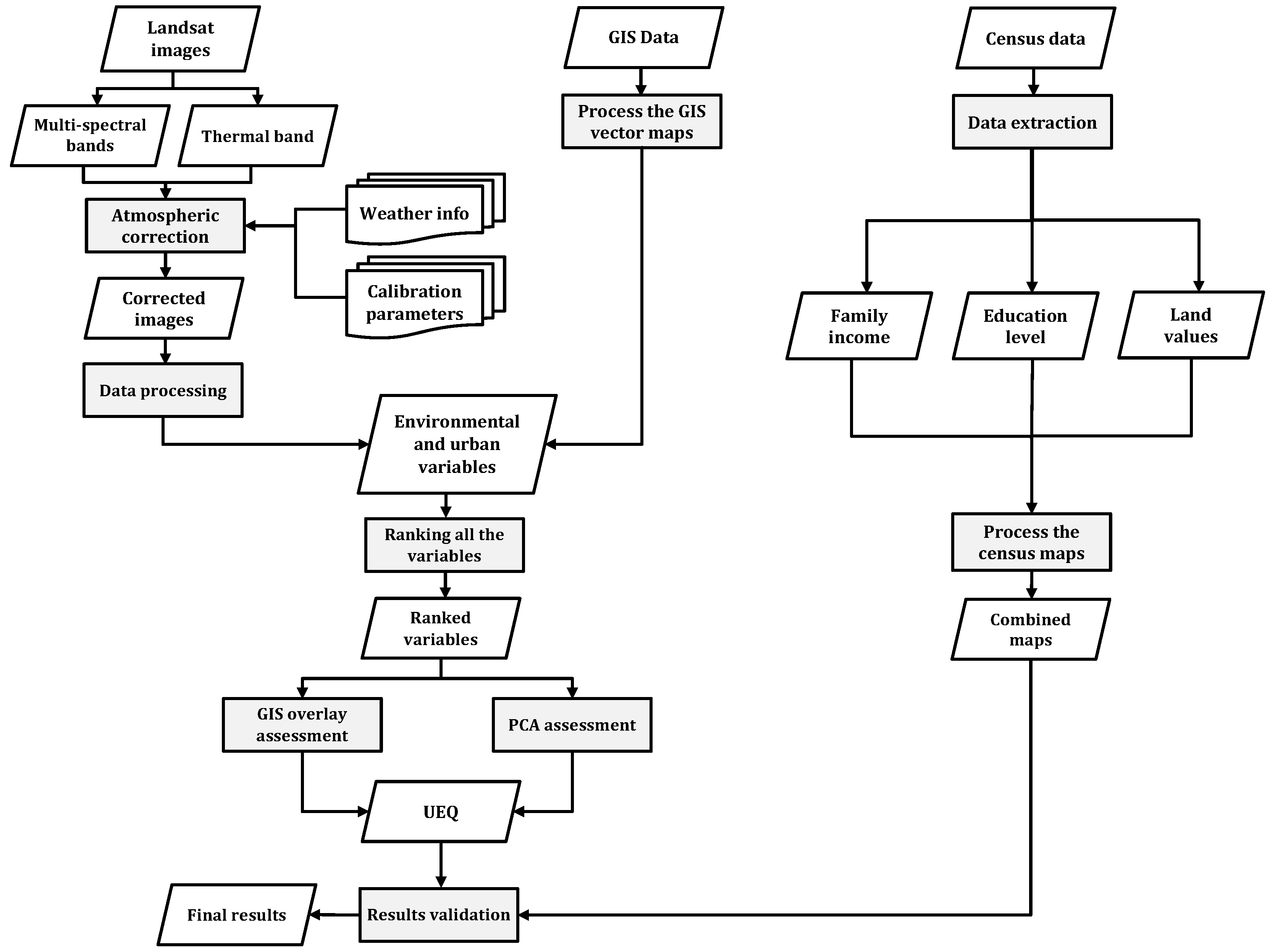
In this research, the main objectives are: (1) to investigate GIS overlay and PCA techniques to assess UEQ with a case study in the city of Toronto, Ontario, Canada; (2) to test a new approach to normalize the data derived from remote sensing and GIS data; and (3) to assess a new approach to validate the final outcomes derived from GIS overlay and PCA. Thus, various remote sensing and GIS data were first explored in order to fully understand the concept of UEQ. The urban, environmental and socio-economic parameters were normalized in this research in order to evaluate the significance of each parameter. GIS overlay and PCA (pixel-based and object-based) were introduced to integrate the urban, environmental and socio-economic parameters with a case study in Toronto. Socio-economic parameters, including family income, degree of education and land value, were used as a reference to validate the outcomes derived from the two integration methods.

2. Datasets

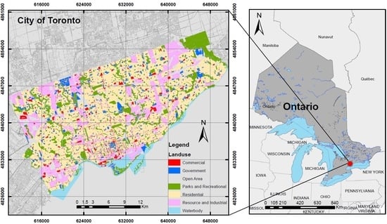
In this research, the city of Toronto, Ontario, Canada, was intentionally selected due to the data availability and the drivers of the population growth within the city during the past decade. Figure 1 shows Toronto, which is the capital of the Province of Ontario and the largest city in Canada with a total population of 2,615,060 [18]. The datasets being used in this study include three major categories: (1) Landsat TM satellite images; (2) GIS data layers; and (3) socio-economic data. All of the data were collected in the years 2010 and 2011, since GIS data and socio-economic are not consistently available after the year 2011. A Landsat TM image was downloaded from the United States Geological Survey (USGS) Earth Explorer [19]. The spatial resolution of the Landsat images is 30 m for the multi-spectral bands and 120 m for the thermal band. However, the thermal band was resampled to a 30-m resolution from the source of the data predominantly to align it with the multi-spectral bands [20]. The image was acquired during the summer season (July) in order to avoid the appearance of clouds and snow cover. On the other hand, a total of 14 GIS data layers were acquired from the Scholars GeoPortal [21] for Toronto during the same period of time. The GIS layer data including land use, population density, building density, vegetation and parks, public transportation, historical areas, Central Business District (CBD), sports areas, religious and cultural zonse, shopping centres, education institutions, entertainment zones, crime rate and health condition. These layers were first imported into the ArcGIS platform (ArcGIS; Esri; Redlands, CA, USA) for further analysis. Similar to the remote sensing data, all of the data were projected to the Universal Transverse Mercator (UTM) 17 N coordinate system. Those social-economic parameters were derived based on the use of Toronto census data that were obtained from the City of Toronto census bureau at the census tract level. The City of Toronto census bureau archives hundreds of information related to socio-economic conditions. In this research, the socio-economic parameters included education (university certificate, diploma or degree), family income and land values. Table 1 summarizes the data sources being used in this study.

3. Methodology

Figure 2 shows the overall workflow implemented in this research. The Landsat image was clipped to the study area to speed up the data processing. The Atmospheric Correction model (ATCOR2) developed by Richter [22] was utilized to preform radiometric calibration and remove the effects that change the spectral characteristics of the land features [23]. To implement the ATCOR2 model, weather information (e.g., air temperature, visibility, etc.) was obtained from historical records at the nearest weather station at Lester B. Pearson International Airport.
The calibration parameters for Landsat TM sensor (biases and gains) were also incorporated into the atmospheric correction. After conducting the atmospheric correction, those bio-physical parameters, including NDVI, NDWI, built-up index and LST, were derived from the Landsat images. Urban, environmental and socio-economic parameters were all extracted from the remote sensing, GIS and census data to combine all of the parameters together in the subsequent process. GIS overlay and PCA (pixel-based and object-based approach) were implemented, respectively, to integrate all of the urban, environmental and socio-economic parameters. Socio-economic parameters obtained from the City of Toronto census bureau, including family income, higher education level and land values, were used as a reference to assess the outcomes from GIS overlay and PCA. The validation was based on two criteria, including precision and accuracy (refer to Section 3.5.3). The final stage of the work is to assign the optimal integrated method to determine the best UEQ location in Toronto.

3.1. Environmental Parameters

3.1.1. Land Surface Temperature (LST)

LST is an essential parameter in a variety of disciplines used to study the urban climate [24,25], UEQ [8], urban heat island effect [26], urban expansion [27] and urban waste management [28]. LST is the result of a land-surface process that combines the analysis of all surface-atmosphere interactions and energy fluxes between the atmosphere and the ground. Mapping the LST from thermal remote sensing sensors can be useful for large-scale environmental and urban studies. Landsat TM and ETM+ data were substantially used in many urban environmental quality studies to derive the LST [2,3,4]. Landsat TM and ETM+ both have: (1) an archive of images that was released free to the public by the USGS [19] in 2008 and (2) a short repeat cycle (16 days), which produces a voluminous data archive for multi-temporal studies. Numerous researchers discussed the use of LST and the challenges to retrieve the LST using known and unknown Land Surface Emissivity (LSE) [29,30]. In this research, the authors utilized Geomatica (Geomatica, version 10.1; PCI Geomatics, Markham, ON, Canada, 2007). to derive the LST from the Landsat images. The adopted method to derive the LST in this research takes into consideration the atmospheric correction of the thermal band of the image. The computation of LST mainly involves three steps. The first step is to convert the pixel value of the thermal band into radiance using the following Equation (1):
L s a t = L m a x L m i n ( Q c a l . m a x Q c a l . m i n ) ( Q c a l Q c a l . m i n ) + L m i n
where L s a t is the spectral radiance; L m a x is the spectral radiance that is scaled to Q c a l . m a x ; L m i n is the spectral radiance to Q c a l . m i n ; Q c a l is the quantized calibrated pixel value in a digital number; and Q c a l . m a x is the maximum quantized calibrated pixel value corresponding to L m a x . For Landsat TM Band 6, the values for L m a x , L m i n and Q c a l . m a x are 15.3032 Wm 2 ·sr 1 · μ m 1 , 1.2378 Wm 2 ·sr 1 · μ m 1 and 255, respectively.
The second step is to compute the emissivity value. Many factors, including water content, chemical composition, structure and roughness, are able to affect the emissivity of a surface [31]. Scholars emphasized that the surface temperature calculation mainly relies on an assumption of the emissivity value [32]. Some researchers assumed the emissivity value as a constant value (0.95) [33]. In contrast, other researchers epitomized that a constant emissivity value can be considered as an option and assigned three classes for the emissivity values, where the vegetation has ϵ = 0.97 , soil ϵ = 0.96 and others ϵ = 0.98 as a rule of thumb [32]. However, if the emissivity value is unknown, the following Equation (2) can be used to calculate the emissivity value [34]:
ϵ = a + b × l n ( N D V I )
where a and b are obtained by a regression analysis based on a large dataset [35]. NDVI is the Normalized Difference Vegetation Index, which can be calculated from the values of the visible and near-infrared bands of the multi-spectral bands, as shown in Section 3.1.2.
The third step is to conduct the atmospheric correction for the thermal band using the following Equation (3). As mentioned in Section 3, weather information (e.g., air temperature, visibility, etc.) and date and time, latitude and longitude are also needed to implement atmospheric correction. The equation for the atmospheric correction can be written as [36]:
L C = L s a t L u p ϵ × τ 1 ϵ ϵ × L d
where L C is the atmospherically-corrected radiance, L s a t is the spectral radiance (Wm 2 ·sr 1 · μ m 1 ), L u p and L d are the upwelling and downwelling radiances (Wm 2 ·sr 1 · μ m 1 ) and ϵ and τ are the emissivity and transmittance, respectively.
The fourth step is to convert the calibrated radiance into the at-sensor brightness temperature using the following Equation (4):
L B B T = K 2 l n ( K 1 L C + 1 )
where T B B T is the blackbody temperature in Kelvin (K), K 1 is the calibration Constant 1 in Wm 2 ·sr 1 · μ m 1 and K 2 is the calibration Constant 2 in Kelvin (K). For Landsat TM, K 1 and K 2 are 607.76 Wm 2 ·sr 1 · μ m 1 and 1260.56 K, respectively [37].
The fifth step is to convert temperature from Kelvin into temperature in Celsius using the following Equation (5):
° C = L B B T 273.15
The computed ( ° C) is regarded as the LST derived from the Landsat image.

3.1.2. Normalized Difference Vegetation Index (NDVI)

Prior to the existence of satellite remote sensing, urban vegetation was usually monitored and mapped by combining colour infrared aerial images and fieldwork. This method seems to be a unique option to measure the urban vegetation [38]. With the availability of multi-source multi-spectral satellite images, Fung and Siu [10] used Landsat and SPOT (Satellite Pour l’Observation de la Terre; Satellite for the Observation of Earth; Spot Image, Toulouse, France) images to quantify urban vegetation as a parameter for UEQ studies. Many researchers used Landsat images to extract NDVI [2,8,39]. NDVI is a ratio that presents the changes in the vegetation over time, and it has been applied to various applications, such as vegetation cover, biomass and Leaf Area Index (LAI) [40,41]. Most of the urban environmental studies showed that NDVI is one of the most important parameters that can be used to assess UEQ, where the higher values represent the positive impact on the city [2,8]. The NDVI (ranging from −1 to 1) refers to an index that is able to monitor the vegetation activity and its annual changes, which can be calculated using Equation (6) [42]:
NDVI = N I R R e d N I R + R e d
where N I R is the near infrared Band 4 in the Landsat TM image and R e d is the red Band 3 in the Landsat TM image.

3.1.3. Normalized Difference Vegetation Index (NDWI)

NDWI is another remote sensing-derived biophysical parameter that represents the surface moisture in vegetation cover, as well as water bodies. Hardisky et al. [43] found that NDWI is able to track changes in vegetation biomass and water stress more than NDVI. NDWI can also be used to measure and assess the turbidity of water bodies from remote sensing data [44], and therefore, Liang and Weng [11] used NDWI as a parameter to assess the UEQ where the higher NDWI represents the higher urban quality (i.e., close to lake shore). The NDWI (ranging from −1 to 1) can be are calculated using Equation (7) [14]:
NDWI = G r e e n N I R G r e e n + N I R
where N I R is the near infrared Band 4 in the Landsat TM image and G r e e n is the green Band 2 in the Landsat TM image.

3.1.4. Normalized Difference Built-Up Index (NDBI) and Built-Up Index

NDBI is another ratio that represents the spatial distribution of the urban and suburban areas. NDBI has been used in many urban planning applications. Zha et al. [42] used the combination of NDBI and NDVI to identify and monitor the areas in the city of Nanjing. Chen et al. [45] shows that land cover types can be represented by utilizing NDVI, NDWI and NDBI. Moreover, Faisal and Shaker [46,47] show that the built-up index derived from NDBI and NDVI could represent industrial areas within the city. Therefore, in UEQ studies, the higher NDBI/built-up values may be deemed to have a negative impact on the city. To derive the built-up area, first, the NDBI values (ranging from −1 to 1) are calculated using Equation (8) [42]:
NDBI = M I R N I R M I D + N I R
where M I R is the mid-infrared Band 5 of the Landsat TM image and N I R is the near infrared Band 4 of the Landsat TM image. The NDBI values refer to an index that represents the urban regions and its annual changes. Finally, the built-up values (ranging from −1 to 1) are defined by subtracting the NDBI layer from the NDVI layer using the following Equation (9) of Zha et al. [42]:
Built up area = N D B I N D V I

3.2. Urban Planning Parameters

3.2.1. Land Use and Land Cover

The expansion of population can affect the urban environment and urban planning around the world. Therefore, monitoring land use and land cover should be conducted to avoid potential problems for sustainable urban and environmental planning. Monitoring land use and land cover helps planners and decision makers to build better urban environmental cities in the near future and assess the quality of the urban cities. Various studies recommended building urban green cities rather than a dense high rise urban environment. Urban green cities increase the value of UEQ within the city [48,49,50]. Medium to fine-scale land cover and land use maps can be derived from remote sensing satellite images [51] or, recently, airborne LiDAR data [52]. However, the accuracy of land cover and land use can change from one satellite to another due to the variation of the spatial resolutions of the satellites. In order to assess the urban quality of living, physical environmental parameters should be obtained. Physical environmental parameters, such as roads, cropland and pasture, water, commercial and industrial, high density residential, medium density residential, low density residential, forest and grass, are critical and essential parameters to assess the urban quality of life. The physical environmental parameters can be used also to extract some of the socio-economic parameters, such as population density and social conditions [11].

3.2.2. Urban Density

Around the world, residential areas can be affected by the increase of population and migration movement. Building density is one of the most important parameters that contributes to the urban heat island effect and urban quality assessment [53]. Building and population density can have a negative influence on the UEQ and transportation system in the developing cities. That is mainly because a dense high rise urban environment typically increases LST, noise pollution together with a high demand of vehicle use [54]. However, most public services, public transportation and jobs are located within walking distance from high density areas. Remote sensing technique can aid in determining the density values by extracting the urban areas from the image [8,12]. The extracted urban areas can be divided by the total areas, so as to calculate the building density, as shown in Equation (10). On the other hand, the population density can be calculated by dividing the number of people over the urban area as shown in Equation (11):
Building density = Urban   areas Total   areas
Population density = Number   of   people Urban   areas

3.2.3. Public Transportation

The acceleration of population growth may increase car ownership, which may increase the amount of carbon dioxide emission and subsequently affect the accessibility to roads, especially in the developing countries [55]. Transportation is the main sector that works in shaping and connecting the cities. Public transportation provides a faster, safer and easier way to travel around the city. Public transportation can help the city through connecting the sub-centres around the railway stations and building a linear development along the route of the public transit line [55]. It was found that most of the automobile-dependent cities lose the traditional community support processes [55]. Therefore, public transportation is one of the major parameters for the UEQ.

3.2.4. Open Spaces and Entertainment Zones

Many studies in UEQ justified that open spaces and open green areas are significant factors contributing to high environmental quality areas [8,12]. That is mainly because open spaces and parks offer a healthy and comfortable environment by cooling down the LST and reducing the air pollution especially in high density areas. Entertainment areas are mainly located in the public parks, plazas and open space areas for some occasions, such as Christmas and New Year. Famous open spaces, such as Times Square in the city of New York, Dundas square and Nathan Phillips Square in Toronto, are so invigorating with a big amount of visitors all over the year, mainly because they are located within the core of high density areas and thus provide a vibrant atmosphere. Such a phenomenon supports the argument that high density areas are more preferable than low density areas.

3.2.5. Historical Areas and Central Business Districts (CBD)

The design of historical cities around the world is mainly based on walking distance. Those historical cities are usually featured by high density, mixed land use and shaded streets in central forms, such as Jerusalem, Damascus, Athens and Istanbul. The average walking distance toward the historical cities is designed to be 5 km apart in order to be close to other facilitates in the city. A few cities still currently retain the historical buildings and walking characteristics, such as Society Hill in Philadelphia, the North End in Boston and the Rocks in Sydney [55]. That is mainly because historical areas retrieve the worth of past energy and provide a visual and physical conservation of cultural identity [56]. Currently, modern cities have more of a tendency to rebuild and preserve historical areas, such as Arabella Park in Munich, to attract tourists and provide a vibrant atmosphere for the city [55]. Historical neighbourhoods, which are always located in the city centre, have higher positive influence on UEQ, where the historical neighbourhoods and CBD are the most attractive regions in the city.

3.2.6. Crime Rate

Personal security is one of the most important factors for society regardless of where we live. Crime can be the reason for physical pain, anxiety and the loss of lives and property [57]. Anand and Santos [58] illustrated that the biggest influence of crime is the feeling of vulnerability in people’s lives, and thus, the crime rate is negatively related to UEQ. It was reported that people move to live in more suburban and low density areas for the desire for new and better public schools and a low crime rate. However, in some cases, the low cost of housing may cause a demand for more housing per person, which may form new clusters for new urban crime [59]. Increasing the physical distance between the poor and the rich is not always the best way to reduce urban crime, particularly in the city centre. Instead, it is preferable to increase the community services and the quality of life in those areas to make them more vibrant and reduce the crime rate [54]. The crime rate can be calculated by dividing the number of crimes over the total population, as shown in Equation (12):
Crime rate = Number   of   crime Total   population

3.3. Socio-Economic Parameters

3.3.1. Education and Income

Education and income are two related factors among relevant socio-economic parameters. Research shows that wealthier urbanites tend to invest more in high quality properties and services. That is mainly because they have higher income and receive higher education, which gives them the tools to access and process more data about the high quality areas. In addition, people with high income and high education have the ability to invest in higher quality areas, compared to people with less education and less income [60]. Moreover, Kahn [54] pointed out that people with higher education and income are more interested in supporting UEQ-related issues. Wealthier and educated urbanites also tend to participate in politics and the community in order to enhance the quality of living in their living areas. Based on the above argument, the areas that have more highly-educated and wealthier urbanites are considered to have higher UEQ areas. Therefore, these areas are used as the first category of reference for our study.

3.3.2. Land Values

Knowing the parameters that influence the UEQ is an important advantage to design and assess the future urban development. UEQ is assessed by using various urban and environmental parameters. Reginster and Goffette-Nagot [61] conducted a study in two Belgian cities to investigate the relationship between the UEQ with respect to the residential location. It was revealed that UEQ may affect positively the land rent location and income in the city. Other research discussed the relationship between the real estate evaluation model and the environmental parameters in the city of Geneva, Switzerland [62]. It was found that urban and environmental parameters have an influence on the price within the city of Geneva. Topcu and Kubat [63] also examined the relationship between urban and spatial factors that might influence the urban land values in the city of Istanbul. It was found that the distance from the sea, the distances from the central business district, universities and sanitary facilities, as well as the the variable of the colour of building facades all have a predominant impact on the residential land values. As a result, our experiment assigned the land values as the second category of reference for this research.

3.4. Ranking the Parameters

Since the aforementioned parameters are extracted from different data sources, they may have different scale levels and cannot be combined to a specific unit. Therefore, all of the obtained data (parameters), including raster, census and GIS data, were first transformed into one scale (sub-neighbour), as shown in Figure 3. Then, all of the parameters were ranked from 1 to 10 to normalize the observation value for each parameter.
To normalize the parameters and represent the significant level of each polygon in the parameter, the Z-score method was performed for all parameters. The Z-score model is a statistical measurement that is able to standardize a wide range of data to represent the significant changes across the data [64]. Equation (13) shows the first step to normalize the parameters using the Z-score:
Z i = x i μ σ
where x is the observation values (polygons) (refer to the GIS polygons of the parameters as shown in Figure 4), i is the parameter, μ is the mean value of the parameter and σ is the standard deviation of the parameter.
The second step is to use linear interpolation to rank the parameters from 1 to 10 as shown in Figure 5. The polygon within the parameter that has a high Z-score number will represent high values, for example 10. The polygon that has a low Z-score will result in a value of 1. The following Equation (14) shows how linear interpolation was calculated:
R a n k = ( O b s O b s m a x ) ( R a n k m i n R a n k m a x ) ( R a n k m i n R a n k m a x ) + R a n k m a x
where O b s is the current observation value, O b s m a x is the maximum observation value, O b s m i n is the minimum observation value, R a n k m a x is the maximum ranking value, R a n k is the determined ranking value and R a n k m i n is the minimum ranking value.

3.5. Data Integration of Multiple Environmental and Urban Parameters

Integration techniques can be used to combine remote sensing and GIS data and have been applied for urban modelling and analysis [65]. Previous studies demonstrated two integration techniques, namely PCA and GIS overlay, which are able to combine any type of parameter. In this research, three approaches were demonstrated to integrate the above-mentioned environmental and urban parameters.

3.5.1. Geographic Information System (GIS) Overlay

GIS overlay is a multi-criteria application that uses data layers for specific environmental thresholds. Remote sensing data are presented as digital data in raster format. However, census data are presented in GIS vector format. Remote sensing data can thus be integrated with socio-economic data by converting remote sensing data from raster to vector data [7]. In this research, the GIS overlay integration method was used to combine the urban and environmental parameters in order to serve for the UEQ assessment. All of the parameters were converted from raster to vector data in order to be presented as attribute data, as shown in Figure 3 in Section 3.4. While each parameter has a range of values ranked from 1 to 10, the sum of the data layers can thus present the result of UEQ values. Ranking the parameters was mainly based on the observation values; where the highest value is assigned 10 and the lowest value is assigned 1. However, some parameters, including crime rate, industrial areas and LST, are inversely presented (e.g., the highest crime rate or LST value will be assigned 1, and the lowest crime rate or LST value will be assigned 10), as shown in Figure 5. Then, all of the ranks are summed up to compute the UEQ as shown in Figure 6.

3.5.2. Principal Component Analysis (PCA)

PCA is an analysis technique that compresses the high dimension of data into a lower dimension of data that has most of the variance of the data [14]. PCA is commonly used in many remote sensing applications. The covariance matrix of standard PCA may not be the best option for data that have different measurement units. The correlation matrix can be used instead of the covariance matrix to standardize each parameter to the variance unit or zero mean. In this research, pixel-based and object-based methods were used to assess the UEQ in Toronto. In pixel-based approach, all of the parameters were converted to raster format to extract pixel values for each parameters. Then, the pixel values were used in the PCA model to compute the components that have most of the variance of the data. In object-based PCA, the covariance matrix or correlation matrix mainly is derived from the observation values of the GIS polygons. Then, the covariance matrix or correlation matrix will be used to compute the components in the PCA model to assess the UEQ.

3.5.3. Accuracy Assessment

Several researchers attempted to assess the accuracy of the UEQ results using different methods, including e-mail questionnaires, field-based questionnaires and factor analyses. Regardless of the considerable amount of e-mail questionnaires or field-based questionnaires, both methods require overheads for data collection. In addition, factor analysis used in previous work was preformed using the same parameters that have been incorporated to compute the UEQ, which make it unreliable and biased. Several researchers illustrated that education level, including university certificate or diploma, family income and land values, represents the UEQ in the economic and social aspects [54,60,61,62]. Since there is a lack of ground truth to validate the results, we propose to use these socio-economic parameters for data validation and to assess the UEQ results. All of the observation data of the three socio-economic parameters were normalized to be in the same scale from 1 to 10. Then, the sum of the socio-economic parameters can thus present the result of reference, as shown in Table 2.
In addition, the evaluation of the binary classifiers approach was used to assess the UEQ based on the following two performance measures through data interpretation: precision and accuracy.
Precision ( P ) is a measure that evaluates the probability that a positive outcome is correct using Equation (15):
P = T P T P + F P
Accuracy ( A c c ) evaluates the effectiveness of the classifier by its percentage of correct predictions using Equation (16):
A c c = T N + T P F N + F P + T N + T P
where T P refers to “True Positive”, which means the polygon from the proposed method is located physically in the reference layer; T N refers to “True Negative”, which represents the polygons that are not detected in the proposed method and reference layer; F P refers to “False Positive”, which means that the polygon of the proposed method does not really exist in the reference layer; and F N refers to “False Negative”, which means the reference polygons do not exist in the proposed method. With these three indicators, we assessed the UEQ layer from the results of each proposed method including GIS overlay, and PCA assessed the best method for our datasets.

4. Results and Analysis

4.1. GIS Overlay Analysis

Figure 7 shows the UEQ derived in Toronto using the GIS overlay. The distribution of UEQ in Toronto shows that the highest UEQ zones were found in the zones A, B, C and D in green colour, while the lowest UEQ zones are indicated as red colour in the city. The highest UEQ zones are the consequences of the summation of all of the positive parameters including (high vegetation areas, historical areas, areas supported by public transportation, etc.) that are located within Zones A to D. However, negative values of the parameters, including crime, industrial areas and high LST, are constantly located on the red zones within the city. In contrast, the highest values of UEQ areas were found in the high and moderate density areas, while the lowest values were found in the industrial and low density areas.

4.2. Principal Component Analysis

4.2.1. Pixel-Based PCA

In this section, an analysis was first conducted to investigate the relationship among all of the parameters. In pixel-based PCA, all of the parameters were converted from vector to raster in order to compute the spatial correlation among the parameters. Some parameters, including built-up areas, LST layer, industrial areas and crime rate regions, were reversed in order to avoid any negative values in the correlation matrix. Pearson’s correlation coefficient was computed to investigate the dependence among all of the parameters, which is going to help in the subsequent PCA. Table 3 represents the correlation coefficient matrix among all of the parameters. The green vegetation parameter shows a strong positive relationship with NDVI (0.85), NDWI (0.85), reverse built-up areas (0.81) and reverse LST (0.90), as well as the areas close to water bodies (0.8). The green areas parameter also has a moderate correlation with the reverse industrial areas (0.69) and the reverse crime rate parameter (0.75). On the other hand, NDVI has a strong positive relationship with NDWI (0.98), reverse built-up areas parameter (0.96), reverse LST (0.91), green vegetation (0.85), the areas close to water bodies (0.80), reverse industrial areas (0.84) and the reverse crime rate parameter (0.80). The reverse built-up areas parameter has a strong positive correlation with NDVI (0.96), NDWI (0.96), reverse LST (0.87), green vegetation (0.81) and reverse industrial areas (0.83). The areas that are close to water bodies (0.76) and the reverse crime rate parameter (0.80) both have a moderate correlation (0.76 and 0.77), respectively, with the reverse built-up areas parameter. The reverse crime rate parameter has a strong positive relationship with NDVI (0.80), NDWI (0.82), reverse LST (0.79) and the areas close to water bodies (0.82). On the other hand, the reverse crime rate also has a moderate correlation with reverse industrial areas (0.77), reverse built-up areas (0.77), green vegetation (0.75) and the public transportation parameter (0.70). Based on these observations, one can indicate that the high vegetation areas are usually located at low crime rate and low industrial areas within the city. The parameter of low crime rate is also influenced by the transportation within the city because of a high correlation observed between these two parameters. The areas that are covered by public transportation are usually crowded with people, which thus influences the crime rate within the city. These observations also indicate that the reverse built-up areas have a high correlation with industrial areas, which could help to derive the industrial areas using remote sensing data. The high correlation between the parameters may cause redundancy and slow down the processing steps. Therefore, data reduction can help to improve the data processing and cost.
Four components were extracted from all of the parameters using the pixel-based PCA approach. Figure 8 shows the UEQ derived using the pixel-based PCA method. PC1 represents the largest percentage of the variance of the data, with 95% of the total variance. However, the combination of Components 2, 3 and 4 contains only 5% of the total variance. Due to the higher variance of Component 1, it represents most of the parameters, including crime rate, NDVI, NDWI, reverse LST, areas close to water bodies, reverse industrial areas, reverse built-up areas, green vegetation and public transportation parameter, as shown in Table 4. The low variance found in Components 2, 3 and 4 showed that the used pixel-based PCA relied only on the first components, as shown in Figure 9.

4.2.2. Object-Based PCA

In the object-based approach, the polygons of each parameter were used in the PCA model to assess the UEQ. Table 5 represents the correlation coefficient matrix among all of the parameters. Population density has a moderate positive correlation coefficient with the historical areas parameter (0.66), where building density has a moderate negative correlation with green vegetation (−0.61), NDVI (−0.68), NDWI (−0.67) and a positive correlation with built-up areas (0.67) and LST (0.78). NDVI has a strong positive relationship with NDWI (0.88) and a moderate negative correlation with green vegetation (0.66). However, NDVI has a high negative correlation with the built-up areas parameter (−0.90) and LST (-0.80) and also has a moderate negative correlation with building density (−0.68). The built-up areas parameter has a strong positive correlation with building density (0.67) and LST (0.79). In addition, the built-up areas parameter has a negative correlation with NDVI (−0.90) and NDWI (−0.89). NDVI has a very high correlation with NDWI and a negative correlation with the built-up areas parameter and LST, as well as having a moderate negative correlation with building density, which indicates that high NDVI values represent low LST and low high building density areas with more green areas. As mentioned in the previous section, data reduction can improve the data processing and cost. Therefore, the object-based approach was used to reduce the size of the data.
In this study, five components were extracted in the object-based PCA approach, which have eigenvalues larger than one, as shown in Figure 10. The total variance of the five components is 75% of the overall variance of the data. Preliminary analysis revealed that Component 1 has 36% of the total variance of the dataset. Component 1 shows strong positive loadings with NDVI (0.88), NDWI (0.86), building density (0.80), LST and historical areas (0.86) and strong negative loadings with LST (−0.86) and built-up areas (−0.86). In addition, Component 1 is the best to represent the green areas within the city. Component 2 reveals about 16% of the dataset, which mainly represents industrial areas with a positive correlation of 0.63 and CBD with a positive correlation of 0.76. Component 2 can be used to represent more about the urban areas. Component 3 represents 9% of the dataset, which mainly represents only sports areas with a positive correlation of (0.81). Component 4 reveals 7% of the dataset, which mainly represents public transportation with a positive correlation of 0.70. Table 6 shows the overall map produced from Components 1 to 5, which represents 75% of the overall variance in the data.

4.3. UEQ Validation Results

As mentioned in the previous section, four socioeconomic parameters were derived from census data. The combination of education level, family income and land values was used to validate the UEQ results. The evaluation of binary classifiers approach was used to evaluate the UEQ, as mentioned in Section 3.5.3. The results of GIS overlay and PCA (pixel-based and object-based) were validated using socioeconomic parameters as a reference for this study. Since we are looking to highlight the higher UEQ areas, the mean values were used as a threshold to derive the higher UEQ areas. Figure 11 shows the reference layer and the high value of the reference layer. The distribution of the reference layer revealed that the highest values are found in the city centre, the west portions of the city, while most of the low UEQ values are found in the east and down town of the city. Figure 12 shows the GIS overlay analysis and the higher values of GIS overlay. There exist a few areas having high UEQ values located in the north and east of the city. The precision and accuracy measured were found to be 71% and 65%, respectively, for the GIS overlay method. That is mainly because the GIS overlay method uses all of the parameters where some of the parameters may have a negative correlation with the reference layer, which may influence the overall result. Figure 13 shows higher UEQ ranking derived using the pixel-based PCA method. The highest values of pixel-based PCA are mainly located in the centre, north, northwest and northeast portions of the city. Since the pixel-based PCA used 95% of the data, the result of the pixel-based PCA shows lower precision and accuracy with respect to GIS overlay. The precision and accuracy are reported to be 68% and 63%, respectively, for pixel-based PCA. Apparently, the pixel-based PCA reveals a lower completeness level, precision and accuracy than GIS overlay, mainly because the pixel-based PCA considered only nine parameters to generate 95% of the data, and some of these parameters have low correlation with the reference layer. Figure 14 shows the object-based PCA and the higher values of the object-based PCA. The result of the object-based PCA represents high UEQ values in the centre, north, northwest and northeast portions of the city. The overall result of object-based PCA reveals a slightly better precision and accuracy by 1% than the pixel-based PCA method. The main reason why the object-based PCA results were slightly better than the pixel-based PCA is mainly because the object-based PCA method considered five components in the analysis, which have more variation of the parameters. However, only one component was considered in the analysis in pixel-based PCA. One more reason could be because in pixel-based PCA, all of the vector data were converted to raster data. That step may cause a certain loss of spatial information, which may affect the overall results. The overall result of the object-based PCA method yielded a lower precision and accuracy by 1% than the GIS overlay method, as shown in Figure 15, and that is mainly because of the same reason for pixel-based PCA, which is the object-based PCA method used only 75% of the total variance. However, the GIS overlay method used all of the parameters.

5. Conclusions

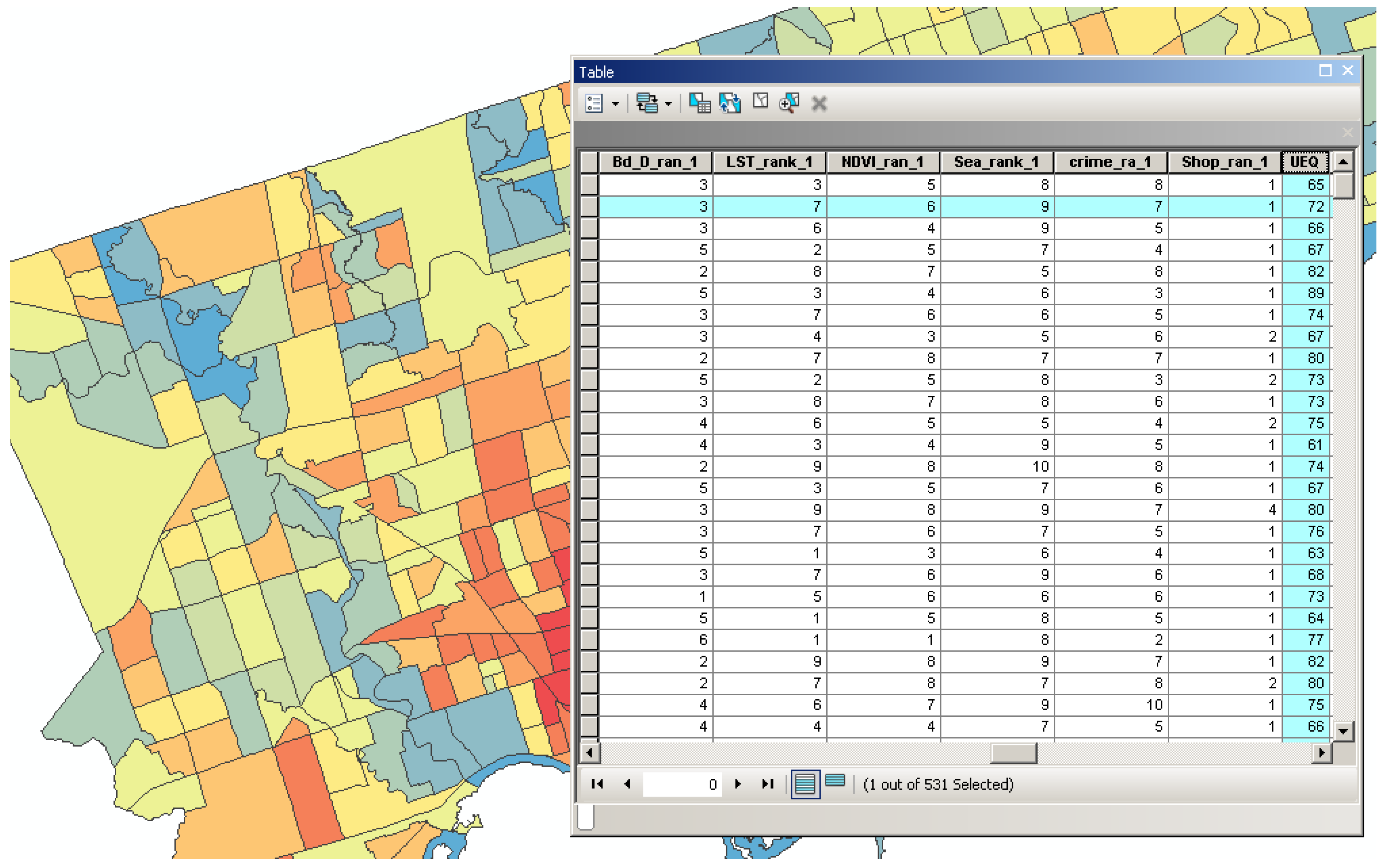
In summary, this study aimed to utilize remote sensing and GIS techniques to assess UEQ with a case study in the city of Toronto, Ontario, Canada, through evaluating two methods: GIS overlay and PCA. One of the issues for the UEQ integration method is that remote sensing, GIS and census data are collected at different scales and in different formats, which may require data normalization before further analysis. In this study, The Z-score model was performed as a first step to normalize all of the parameters. Then, linear interpolation was implemented to rank all of the Z-score values from 1 to 10.
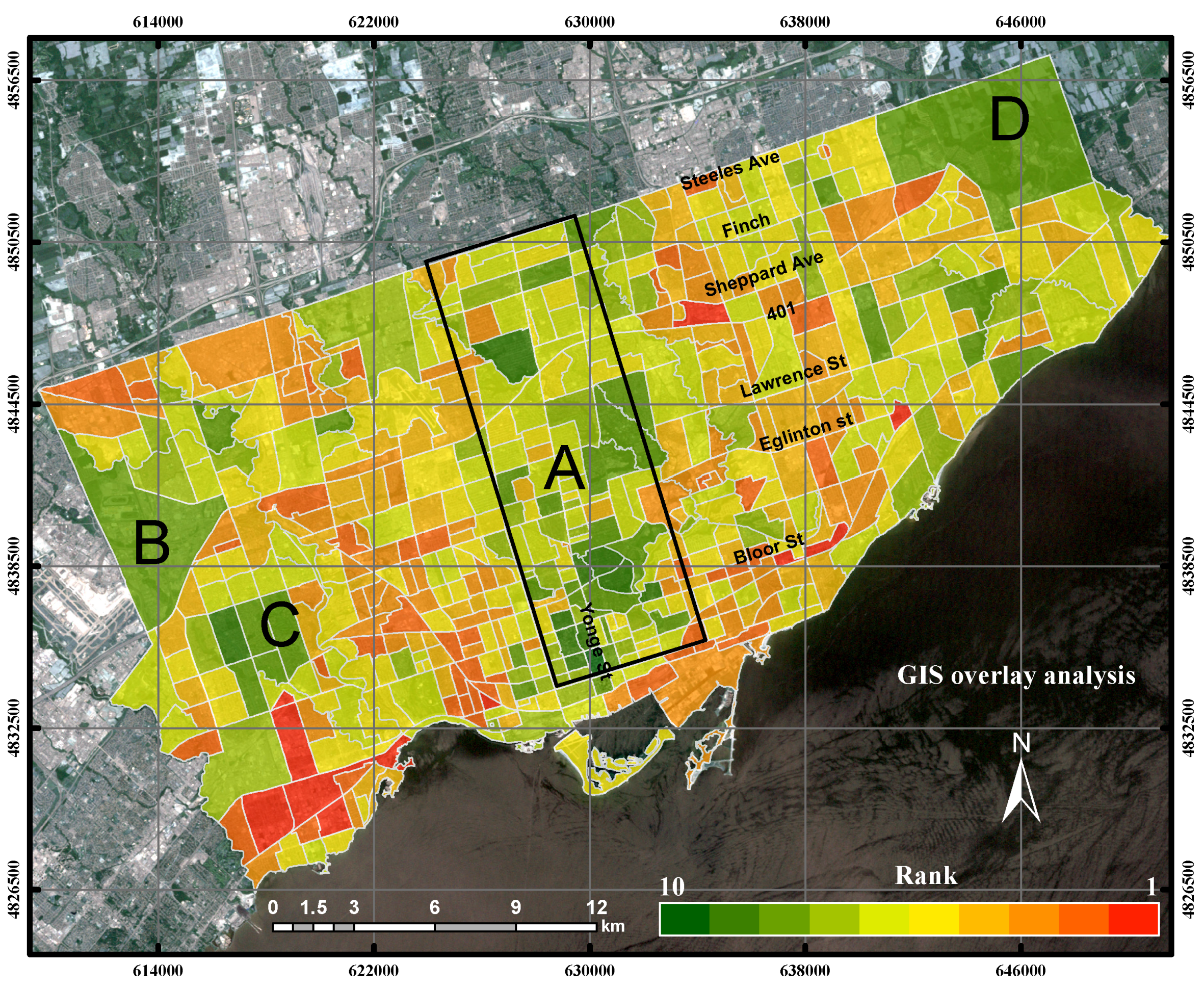
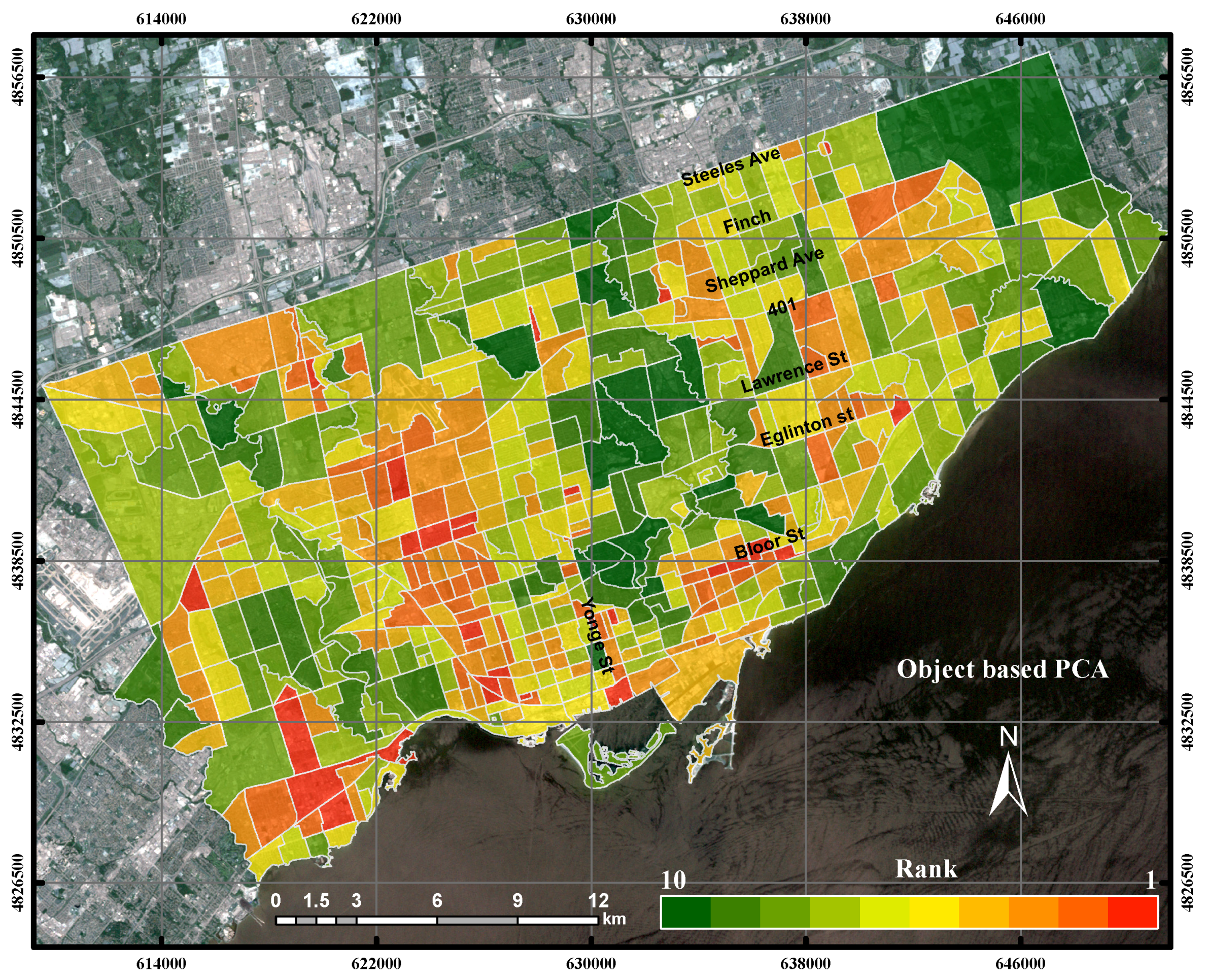
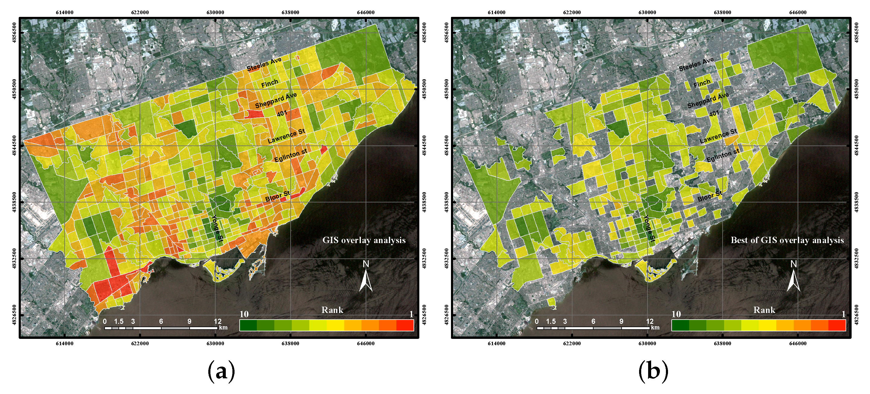
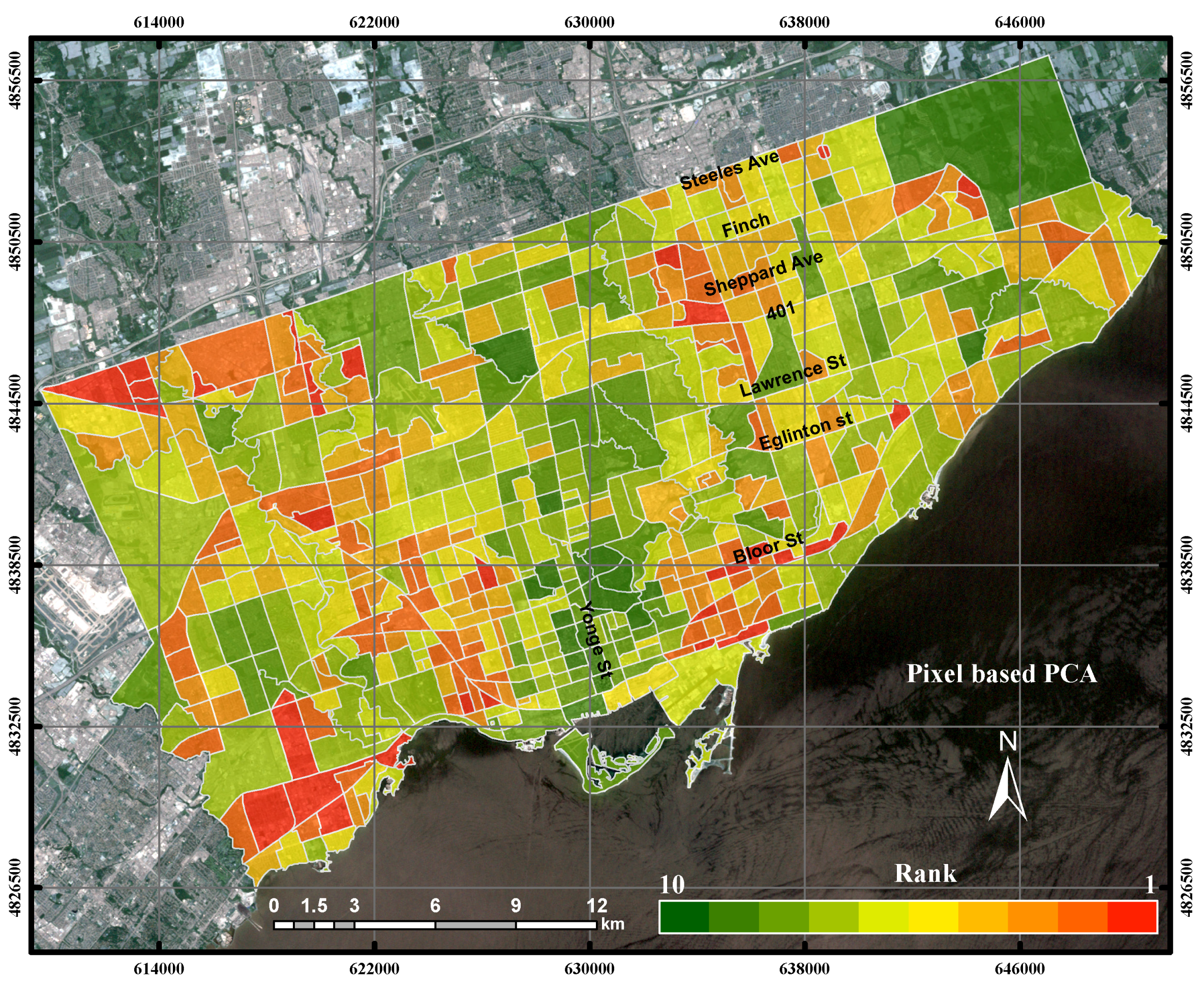
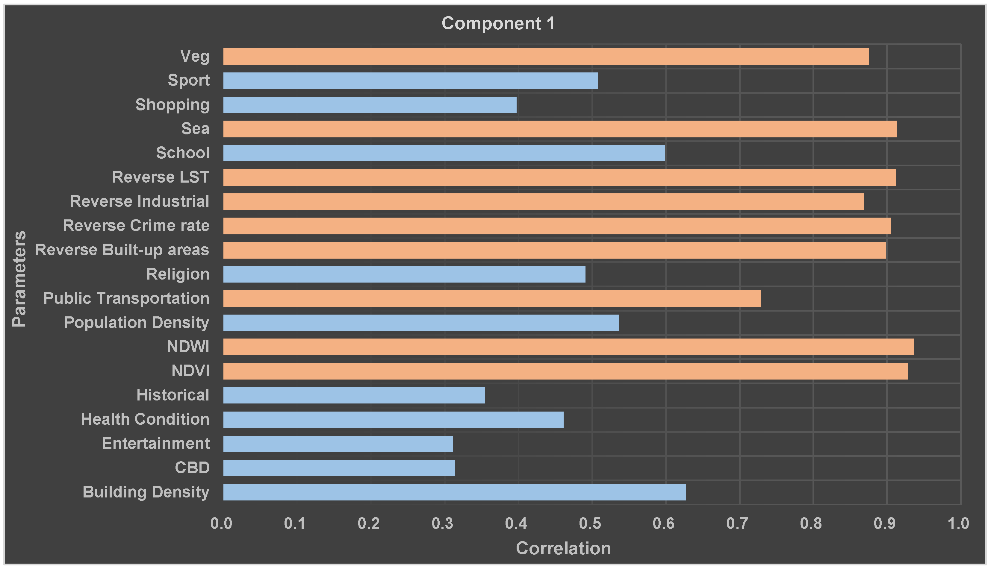
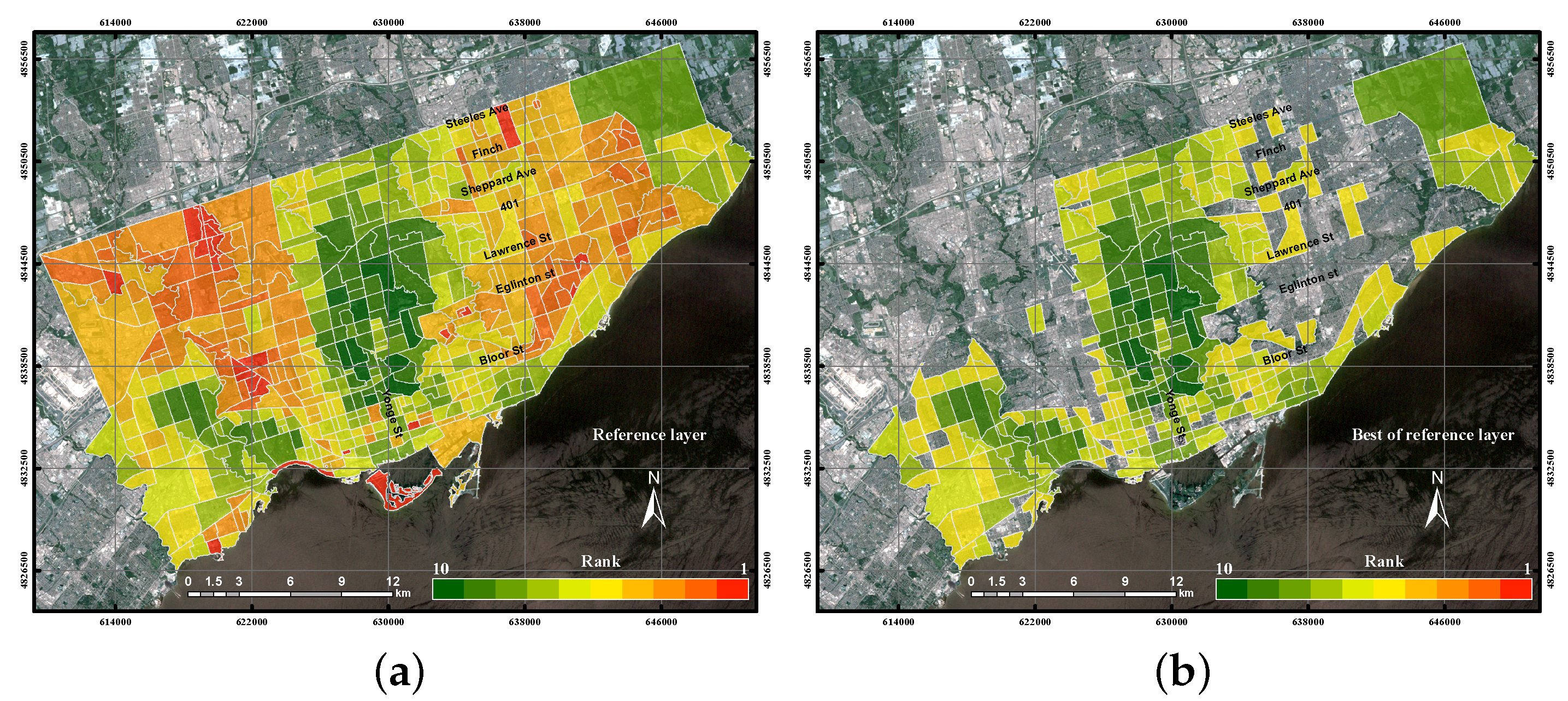
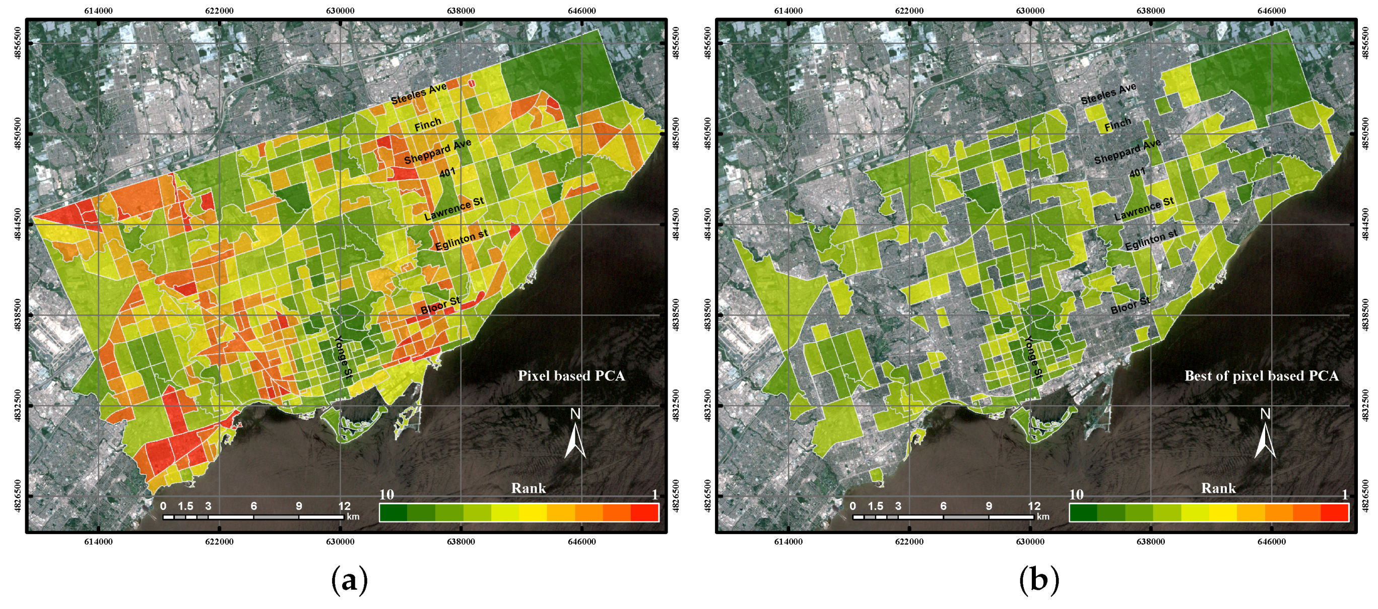
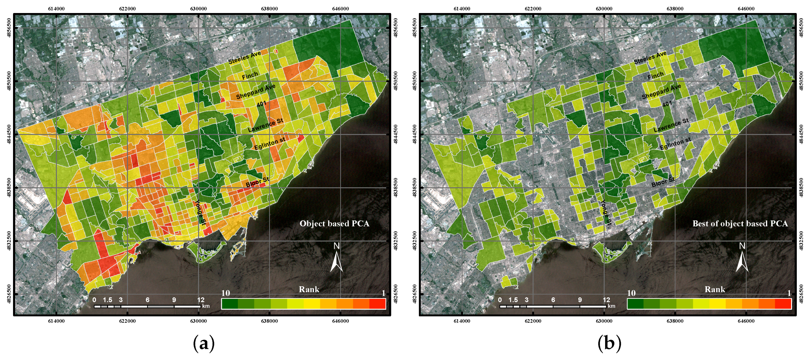
Integration techniques including GIS overlay and PCA (both pixel-based and object-based methods) were used to integrate the environmental, urban and socio-economic parameters. GIS overlay is one of the effective tools for integrating different datasets from different data sources. GIS overlay offers an intelligent platform for creating a comprehensive database to evaluate the UEQ. Correlation analysis investigates the dependence found among urban, environmental and socioeconomic parameters. In our case study, it was found that green areas have a strong positive correlation with NDVI and NDWI. There was a negative relationship with the built-up areas parameter, LST, industrial areas, crime rate and building density. Alternatively, PCA provides an efficient method to reduce the data dimension and redundancy. Four components that have eigenvalues over one were derived from the 19 parameters that represented the urban and environmental aspects in the pixel-based PCA method. Five components that have eigenvalues over one were derived from the 19 parameters that represent the urban and environmental aspects in the object-based PCA method. The two methods (pixel-based and object-based) were tested due to the data availability. Other studies can only consider one method of PCA, since they do not have significant contrast in the results with respect to UEQ parameters.
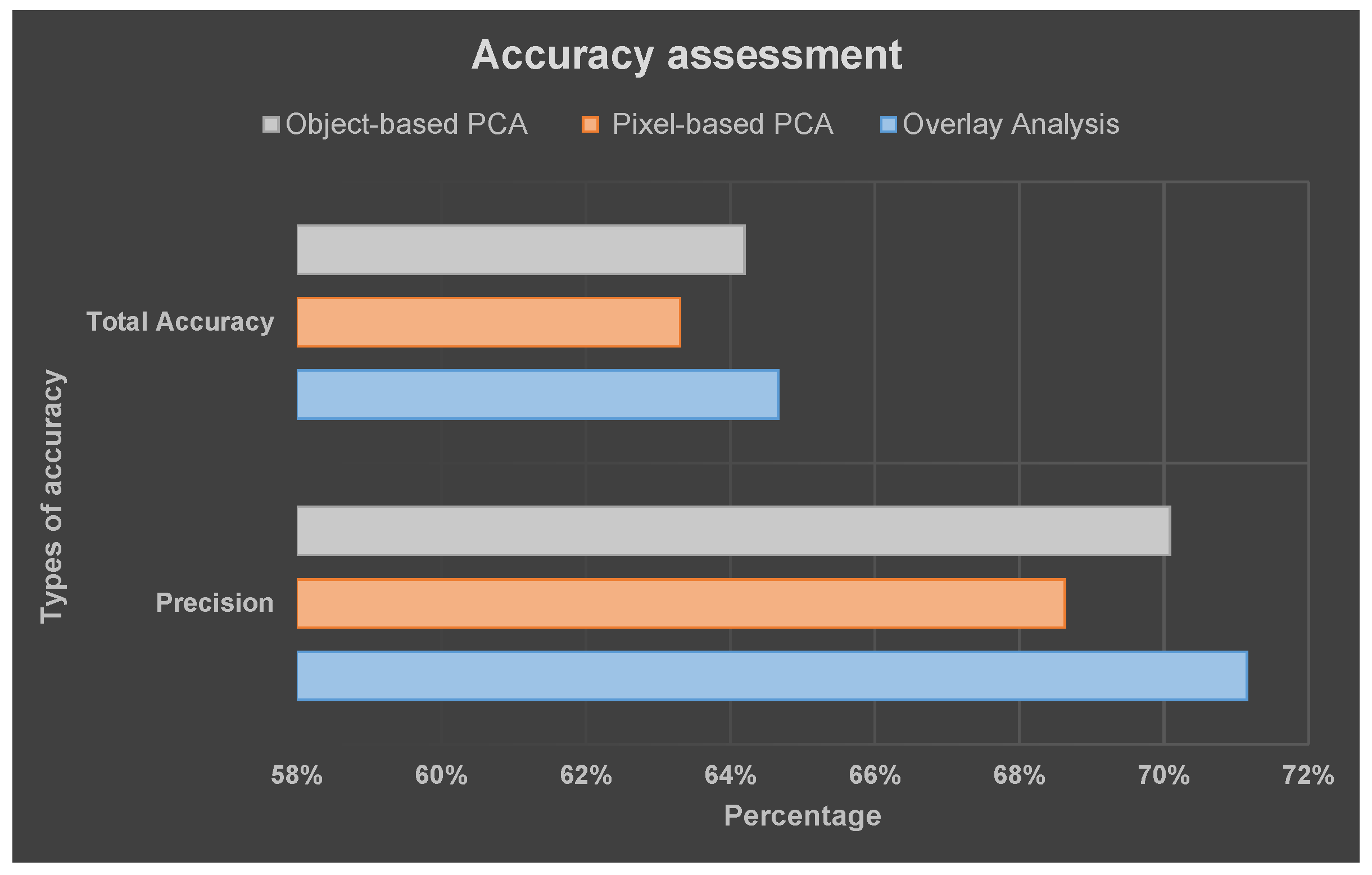
One of the key concerns in UEQ research is to validate the final results derived from different socio-economic references. Despite that some of the existing UEQ studies utilized email or questionnaire surveys to collect the public’s opinion for UEQ assessment, this study proposed to use three socio-economic parameters (university certificate or diploma, family income and land values) as a reference for result assessment. The results showed that the precision was 71% for the GIS overlay method, and the accuracy was measured as 65%. The precision level of the pixel-based PCA method yielded 68%, and the accuracy was reported to be 63%, respectively. The precision level of the object-based PCA was 70%, where the accuracy was reported to be 64%. In this study, GIS overlay represented better results than PCA (pixel-based and object-based) with respect to the UEQ results parameters, which may suggest that GIS overlay can be a better method in terms of the integration of multiple parameters.
Although the presented approach can be used by any federal authorities and municipalities in developing and developed countries, where there is a need to improve and design the new areas within the city, there are a few recommendations for similar future studies: (1) more up-to-date remote sensing and GIS data are required to consolidate the findings; (2) census socioeconomic data usually relate to administrative units and can be changed in a shorter period of time, which makes it difficult to be available worldwide; (3) integration among remote sensing, GIS and socioeconomic data needs conversion between data, such as from raster to vector or from vector to raster, a step that may cause a certain loss of spatial information. To conclude, remote sensing and GIS techniques can provide fruitful information to model UEQ. However, other urban and environmental parameters, as well as empirical models (such as different geographically-weighted approaches) should be considered in order to develop a more universal indicator to predict the UEQ. As a result, further research is under way to study different approaches to narrow down the variety of parameters, as well as developing a new technique to retrieve the UEQ in different cities located in Canada.

Acknowledgments

This research was supported by the Natural Sciences and Engineering Research Council of Canada (NSERC) Discovery Grant. Kamil Faisal acknowledges King Abdul-Aziz University and the Saudi Culture Bureau for the financial support of his Ph.D. study. Special thanks also are extended to Wai Yeung Yan and Dan Jakubek from Ryerson University, who provided technical support and the provision of all of the GIS data, respectively. The authors also acknowledge the United States Geological Survey (USGS) for the remote sensing data and information provided through the EarthExplorer platform.

Author Contributions

The research was conducted by Kamil Faisal under the supervision of Ahmed Shaker, who designed the experiment, provided technical support and guidance and directly contributed to the results of this article. Kamil Faisal wrote the paper. Both authors have read and approved the final manuscript.

Conflicts of Interest

The authors declare no conflict of interest.

References

  1. Weng, Q.; Quattrochi, D.A. Urban Remote Sensing; CRC Press: Boca Raton, FL, USA, 2006. [Google Scholar]
  2. Nichol, J.; Lee, C. Urban vegetation monitoring in Hong Kong using high resolution multispectral images. Int. J. Remote Sens. 2005, 26, 903–918. [Google Scholar] [CrossRef]
  3. Nichol, J.E.; Wong, M.S. Assessing Urban Environmental Quality with Multiple Parameters. In Urban Remote Sensing; CRC Press: Boca Raton, FL, USA, 2006; pp. 253–268. [Google Scholar]
  4. Nichol, J.; Wong, M.S.; Fung, C.; Leung, K.K. Assessment of urban environmental quality in a subtropical city using multispectral satellite images. Environ. Plan. B Plan. Des. 2006, 33, 39–58. [Google Scholar] [CrossRef]
  5. Green, N.E. Aerial Photographic Interpretation and the Social Structure of the City. Photogramm. Eng. 1957, 23, 89–96. [Google Scholar]
  6. Bederman, S.H.; Hartshorn, T.A. Quality of life in Georgia: The 1980 experience. Southeast. Geogr. 1984, 24, 78–98. [Google Scholar] [CrossRef]
  7. Li, G.; Weng, Q. Measuring the quality of life in city of Indianapolis by integration of remote sensing and census data. Int. J. Remote Sens. 2007, 28, 249–267. [Google Scholar] [CrossRef]
  8. Nichol, J.; Wong, M.S. Mapping urban environmental quality using satellite data and multiple parameters. Environ. Plan. B Plan. Des. 2009, 36, 170–185. [Google Scholar] [CrossRef]
  9. Fung, T.; Siu, W. Environmental quality and its changes, an analysis using NDVI. Int. J. Remote Sens. 2000, 21, 1011–1024. [Google Scholar] [CrossRef]
  10. Fung, T.; Siu, W.L. A study of green space and its changes in Hong Kong using NDVI. Geogr. Environ. Model. 2001, 5, 111–122. [Google Scholar] [CrossRef]
  11. Liang, B.; Weng, Q. Assessing urban environmental quality change of Indianapolis, United States, by the remote sensing and GIS integration. IEEE J. Sel. Top. Appl. Earth Obs. Remote Sen. 2011, 4, 43–55. [Google Scholar] [CrossRef]
  12. Rahman, A.; Kumar, Y.; Fazal, S.; Bhaskaran, S. Urbanization and quality of urban environment using remote sensing and GIS techniques in East Delhi-India. J. Geogr. Inf. Syst. 2011, 3, 62. [Google Scholar] [CrossRef]
  13. Rinner, C. A geographic visualization approach to multi-criteria evaluation of urban quality of life. Int. J. Geogr. Inf. Sci. 2007, 21, 907–919. [Google Scholar] [CrossRef]
  14. Jensen, J.R. Introductory Digital Image Processing, 3rd ed.; Prentice Hall: Upper Saddle River, NJ, USA, 2005. [Google Scholar]
  15. Fobil, J.N.; Kraemer, A.; Meyer, C.G.; May, J. Neighborhood urban environmental quality conditions are likely to drive malaria and diarrhea mortality in Accra, Ghana. J. Environ. Public Health 2011, 2011, 484010. [Google Scholar] [CrossRef] [PubMed]
  16. Moore, G.; Croxford, B.; Adams, M.; Refaee, M.; Cox, T.; Sharples, S. Urban environmental quality: Perceptions and measures in three UK cities. WIT Trans. Ecol. Environ. 2006, 93. [Google Scholar] [CrossRef]
  17. Lo, C. Integration of Landsat Thematic Mapper (TM) Data and US Census Data for Quality of Life Assessment. Int. Arch. Photogramm. Remote Sens. 1996, 31, 431–436. [Google Scholar]
  18. Martel, L. The Canadian Population in 2011, Population Counts and Growth: Population and Dwelling Counts, 2011 Census; Statistics Canada: Ottawa, ON, Canada, 2012. [Google Scholar]
  19. United States Geological Survey. Earth Explorer. 2014. Available online: http://earthexplorer.usgs.gov/ (accessed on 25 April 2014). [Google Scholar]
  20. Kjaersgaard, J.; Allen, R. Loading the Landsat Thermal Band Preprocessed Using the EROS LPGS System; Kimberly R&E Center, University of Idaho: Kimberly, ID, USA, 2009. [Google Scholar]
  21. Scholars GeoPortal. Scholars GeoPortal. 2014. Available online: http://geo2.scholarsportal.info (accessed on 19 April 2014).
  22. Richter, R. Correction of satellite imagery over mountainous terrain. Appl. Opt. 1998, 37, 4004–4015. [Google Scholar] [CrossRef] [PubMed]
  23. Paolini, L.; Grings, F.; Sobrino, J.A.; Jiménez Muñoz, J.C.; Karszenbaum, H. Radiometric correction effects in Landsat multi-date/multi-sensor change detection studies. Int. J. Remote Sens. 2006, 27, 685–704. [Google Scholar] [CrossRef]
  24. Norman, J.M.; Kustas, W.P.; Humes, K.S. Source approach for estimating soil and vegetation energy fluxes in observations of directional radiometric surface temperature. Agric. For. Meteorol. 1995, 77, 263–293. [Google Scholar] [CrossRef]
  25. Czajkowski, K.P.; Goward, S.N.; Mulhern, T.; Goetz, S.J.; Walz, A.; Shirey, D.; Stadler, S.; Prince, S.D.; Dubayah, R.O. Estimating environmental variables using thermal remote sensing. In Thermal Remote Sensing in Land Surface Processes; CRC Press: Boca Raton, FL, USA, 2004; pp. 11–32. [Google Scholar]
  26. Weng, Q.; Lu, D.; Schubring, J. Estimation of land surface temperature–vegetation abundance relationship for urban heat island studies. Remote Sens. Environ. 2004, 89, 467–483. [Google Scholar] [CrossRef]
  27. Huang, W.; Zeng, Y.; Li, S. An analysis of urban expansion and its associated thermal characteristics using Landsat imagery. Geocarto Int. 2015, 30, 93–103. [Google Scholar] [CrossRef]
  28. Yan, W.Y.; Mahendrarajah, P.; Shaker, A.; Faisal, K.; Luong, R.; Al-Ahmad, M. Analysis of multi-temporal Landsat satellite images for monitoring land surface temperature of municipal solid waste disposal sites. Environ. Monit. Assess. 2014, 186, 8161–8173. [Google Scholar] [CrossRef] [PubMed]
  29. Li, Z.L.; Tang, B.H.; Wu, H.; Ren, H.; Yan, G.; Wan, Z.; Trigo, I.F.; Sobrino, J.A. Satellite-derived land surface temperature: Current status and perspectives. Remote Sens. Environ. 2013, 131, 14–37. [Google Scholar] [CrossRef]
  30. Sobrino, J.A.; Jiménez-Muñoz, J.C.; Paolini, L. Land surface temperature retrieval from LANDSAT TM 5. Remote Sens. Environ. 2004, 90, 434–440. [Google Scholar] [CrossRef]
  31. Snyder, W.C.; Wan, Z.; Zhang, Y.; Feng, Y.Z. Classification-based emissivity for land surface temperature measurement from space. Int. J. Remote Sens. 1998, 19, 2753–2774. [Google Scholar] [CrossRef]
  32. Richter, R.; Schläpfer, D. Atmospheric/Topographic Correction for Satellite Imagery; DLR Report DLR-IB; ReSe Applications Schläpfer: Wil, Switzerland, 2016; Available online: http://www.rese.ch/pdf/atcor3_manual.pdf (accessed on 1 March 2017).
  33. Coll, C.; Galve, J.M.; Sanchez, J.M.; Caselles, V. Validation of Landsat-7/ETM+ thermal-band calibration and atmospheric correction with ground-based measurements. IEEE Trans. Geosci. Remote Sens. 2010, 48, 547–555. [Google Scholar] [CrossRef]
  34. Giannini, M.; Belfiore, O.; Parente, C.; Santamaria, R. Land Surface Temperature from Landsat 5 TM images: Comparison of different methods using airborne thermal data. J. Eng. Sci. Technol. Rev. 2015, 8, 83–90. [Google Scholar]
  35. Moran, M.S.; Jackson, R.D.; Slater, P.N.; Teillet, P.M. Evaluation of simplified procedures for retrieval of land surface reflectance factors from satellite sensor output. Remote Sens. Environ. 1992, 41, 169–184. [Google Scholar] [CrossRef]
  36. Barsi, J.A.; Schott, J.R.; Palluconi, F.D.; Hook, S.J. Validation of a web-based atmospheric correction tool for single thermal band instruments. In Optics & Photonics 2005; International Society for Optics and Photonics: San Diego, CA, USA, 2005; p. 58820E. [Google Scholar]
  37. Chander, G.; Markham, B.L.; Helder, D.L. Summary of current radiometric calibration coefficients for Landsat MSS, TM, ETM+, and EO-1 ALI sensors. Remote Sens. Environ. 2009, 113, 893–903. [Google Scholar] [CrossRef]
  38. Nowak, D.J.; Rowntree, R.A.; McPherson, E.G.; Sisinni, S.M.; Kerkmann, E.R.; Stevens, J.C. Measuring and analyzing urban tree cover. Landsc. Urban Plan. 1996, 36, 49–57. [Google Scholar] [CrossRef]
  39. Lo, C.P.; Quattrochi, D.A.; Luvall, J.C. Application of high-resolution thermal infrared remote sensing and GIS to assess the urban heat island effect. Int. J. Remote Sens. 1997, 18, 287–304. [Google Scholar] [CrossRef]
  40. Curran, P.; Steven, M. Multispectral remote sensing for the estimation of green leaf area index [and discussion]. Philos. Trans. R. Soc. Lond. A Math. Phys. Eng. Sci. 1983, 309, 257–270. [Google Scholar] [CrossRef]
  41. Lawrence, R.L.; Ripple, W.J. Comparisons among vegetation indices and bandwise regression in a highly disturbed, heterogeneous landscape: Mount St. Helens, Washington. Remote Sens. Environ. 1998, 64, 91–102. [Google Scholar] [CrossRef]
  42. Zha, Y.; Gao, J.; Ni, S. Use of normalized difference built-up index in automatically mapping urban areas from TM imagery. Int. J. Remote Sens. 2003, 24, 583–594. [Google Scholar] [CrossRef]
  43. Hardisky, M.; Klemas, V.; Smart, R.M. The influence of soil salinity, growth form, and leaf moisture on the spectral radiance of Spartina alterniflora canopies. Photogramm. Eng. Remote Sens. 1983, 49, 77–83. [Google Scholar]
  44. McFeeters, S.K. The use of the Normalized Difference Water Index (NDWI) in the delineation of open water features. Int. J. Remote Sens. 1996, 17, 1425–1432. [Google Scholar] [CrossRef]
  45. Chen, X.L.; Zhao, H.M.; Li, P.X.; Yin, Z.Y. Remote sensing image-based analysis of the relationship between urban heat island and land use/cover changes. Remote Sens. Environ. 2006, 104, 133–146. [Google Scholar] [CrossRef]
  46. Faisal, K.; Shaker, A.; Habbani, S. Modeling the Relationship between the Gross Domestic Product and Built-Up Area Using Remote Sensing and GIS Data: A Case Study of Seven Major Cities in Canada. ISPRS Int. J. Geo-Inf. 2016, 5, 23. [Google Scholar] [CrossRef]
  47. Faisal, K.; Shaker, A. The use of remote sensing technique to predict Gross Domestic Product (GDP): An analysis of built-up index and GDP in nine major cities in Canada. Int. Arch. Photogramm. Remote Sens. Spat. Inf. Sci. 2014, 40, 85–92. [Google Scholar] [CrossRef]
  48. Irvine, K.N.; Devine-Wright, P.; Payne, S.R.; Fuller, R.A.; Painter, B.; Gaston, K.J. Green space, soundscape and urban sustainability: An interdisciplinary, empirical study. Local Environ. 2009, 14, 155–172. [Google Scholar] [CrossRef]
  49. Landorf, C.; Brewer, G.; Sheppard, L.A. The urban environment and sustainable ageing: Critical issues and assessment indicators. Local Environ. 2008, 13, 497–514. [Google Scholar] [CrossRef]
  50. din Özdemir, A. Urban sustainability and open space networks. J. Appl. Sci. 2007, 7, 3713–3720. [Google Scholar]
  51. Hansen, M.C.; Loveland, T.R. A review of large area monitoring of land cover change using Landsat data. Remote Sens. Environ. 2012, 122, 66–74. [Google Scholar] [CrossRef]
  52. Yan, W.Y.; Shaker, A.; El-Ashmawy, N. Urban land cover classification using airborne LiDAR data: A review. Remote Sens. Environ. 2015, 158, 295–310. [Google Scholar] [CrossRef]
  53. Mira, R.G.; Uzzell, D.; Deus, J.E.R.; Martínez, J.R. Housing, Space and Quality of Life; Ashgate: Farnham, UK, 2005. [Google Scholar]
  54. Kahn, M.E. Green Cities: Urban Growth and the Environment; Brookings Institution Press: Washington, DC, USA, 2007. [Google Scholar]
  55. Newman, P.; Kenworthy, J. Sustainability and Cities: Overcoming Automobile Dependence; Island Press: Washington, DC, USA, 1999. [Google Scholar]
  56. Leask, A.; Fyall, A. Managing World Heritage Sites; Routledge: New York, NY, USA, 2006. [Google Scholar]
  57. Organisation for Economic Co-operation and Development (OECD) Better Life Initiatives. Compendium of OECD Well-Being Indicators; Organisation for Economic Co-Operation and Development: Paris, France, 2011. [Google Scholar]
  58. Anand, P.; Santos, C.; Smith, R. The Measurement of Capabilities. In Arguments for a Better World. Essays in Honor of Amartya Sen; Basu, K., Kanbur, R., Eds.; Oxford University Press: Oxford, UK, 2008; pp. 283–310. [Google Scholar]
  59. Cullen, J.B.; Levitt, S.D. Crime, urban flight, and the consequences for cities. Rev. Econ. Stat. 1999, 81, 159–169. [Google Scholar] [CrossRef]
  60. Becker, G.S.; Mulligan, C.B. The endogenous determination of time preference. Q. J. Econ. 1997, 112, 729–758. [Google Scholar] [CrossRef]
  61. Reginster, I.; Goffette-Nagot, F. Urban environmental quality in two Belgian cities, evaluated on the basis of residential choices and GIS data. Environ. Plan. A 2005, 37, 1067–1090. [Google Scholar] [CrossRef]
  62. Din, A.; Hoesli, M.; Bender, A. Environmental variables and real estate prices. Urban Stud. 2001, 38, 1989–2000. [Google Scholar] [CrossRef]
  63. Topcu, M.; Kubat, A.S. The analysis of urban features that affect land values in residential areas. In Proceedings of the 7th International Space Syntax Symposium, Stockholm, Sweden, 8–11 June 2009; Volume 26, p. 26.
  64. Cheadle, C.; Vawter, M.P.; Freed, W.J.; Becker, K.G. Analysis of microarray data using Z score transformation. J. Mol. Diagn. 2003, 5, 73–81. [Google Scholar] [CrossRef]
  65. Weng, Q. Land use change analysis in the Zhujiang Delta of China using satellite remote sensing, GIS and stochastic modelling. J. Environ. Manag. 2002, 64, 273–284. [Google Scholar] [CrossRef]
Figure 1. City of Toronto (the study area).
Sustainability 09 00380 g001
Figure 2. The overall workflow. UEQ, Urban Environmental Quality; PCA, Principal Component Analysis; GIS, Geographic Information System.
Sustainability 09 00380 g002
Figure 3. (a) NDVI image derived from Landsat image (raster data); (b) NDVI map after transformation (vector data); (c) population layer at the census tract level; (d) population layer after transformation to sub-neighbour level.
Sustainability 09 00380 g003
Figure 4. The GIS polygons of the parameters.
Sustainability 09 00380 g004
Figure 5. (a) The LST layer in degrees Celsius before ranking the parameter; (b) the ranking of LST after the normalization.
Sustainability 09 00380 g005
Figure 6. The summed up ranks for all of the parameters.
Sustainability 09 00380 g006
Figure 7. The UEQ derived using the GIS overlay method.
Sustainability 09 00380 g007
Figure 8. The UEQ derived using the first component of the pixel-based PCA method.
Sustainability 09 00380 g008
Figure 9. The UEQ parameters versus PCA Component 1.
Sustainability 09 00380 g009
Figure 10. The UEQ derived using four components of the object-based PCA method.
Sustainability 09 00380 g010
Figure 11. The reference layer and the results of the reference layer higher than the mean. (a) The reference layer; (b) results of the reference layer higher than the mean.
Sustainability 09 00380 g011
Figure 12. The UEQ derived using the GIS overlay method. (a) The derived UEQ; (b) UEQ zones higher than the mean.
Sustainability 09 00380 g012
Figure 13. The UEQ derived using the pixel-based method. (a) The derived UEQ; (b) UEQ zones higher than the mean.
Sustainability 09 00380 g013
Figure 14. The UEQ derived using the object-based method. (a) The derived UEQ; (b) UEQ zones higher than the mean.
Sustainability 09 00380 g014
Figure 15. The UEQ validation.
Sustainability 09 00380 g015
Table 1. The data sources used in this study.
CityLandsat TMGIS DataCensus Data
Path/Row = 18/30◦ Land UseSocio-economic data are provided by the City of Toronto census bureau. Socio-economic data used in the research include:
Sensor = Landsat TM◦ Population Density
Date = 23 June 2011◦ Building Density
◦ Vegetation and Parks
Remote sensing data used in this work:◦ Public Transportation
◦ Historical Areas◦ Education
◦ LST◦ Central Business Districts (CBD)◦ Family Income
Toronto◦ NDVI◦ Sports Areas◦ Land Values
◦ NDWI◦ Religious and Cultural Zones
◦ NDBI and Built-up Area◦ Shopping Centres
◦ Education Institutions
◦ Entertainment Zones
◦ Crime Rate
◦ Health Condition
◦ Areas Close to Water Bodies
LST, Land Surface Temperature; NDVI, Normalized Difference Vegetation Index; Normalized Difference Water Index; NDBI, Normalized Difference Built-up Index
Table 2. The sum of the socio-economic parameters.
Polygon IDIncomeEducationLand ValueReference Layer
185720
Table 3. The correlation coefficient matrix among all of the parameters derived using the pixel-based method.
PDBDPTVegNDVINDWIrBUrLSTHrIndCBDScEntHeRelSPSearCRSH
PD1.000.680.570.330.390.400.420.320.670.520.560.330.460.400.220.330.440.430.42
BD 1.000.620.330.400.420.600.360.480.520.400.430.320.440.450.330.590.600.41
PT 1.000.480.520.540.470.500.310.600.270.410.220.410.410.290.700.700.34
Veg 1.000.850.850.810.900.250.690.250.510.280.350.440.490.800.750.35
NDVI 1.000.980.960.910.210.840.160.520.180.330.330.430.800.800.22
NDWI 1.000.960.910.210.860.170.510.160.320.320.420.810.820.20
rBU 1.000.870.260.830.200.490.170.340.270.420.760.770.22
rLST 1.000.220.750.240.520.250.350.440.460.830.790.31
H 1.000.260.820.390.640.430.310.410.260.210.55
rInd 1.000.220.380.170.300.190.260.760.770.20
CBD 1.000.300.530.350.230.320.280.170.48
Sc 1.000.350.460.620.680.430.510.44
Ent 1.000.370.480.400.240.190.74
He 1.000.370.390.410.350.48
Rel 1.000.580.420.460.57
SP 1.000.380.410.43
Sea 1.000.820.34
rCR 1.000.33
SH 1.00
PD, Population Density; BD, Building Density; PT, Public Transportation; Veg, Vegetation areas; rBU, reverse Built-Up areas; rLST, reverse LST; H, Historical areas; rInd, reverse Industrial areas; Sc, School areas; Ent, Entertainment areas; He, Health condition; Rel, Religion areas; SP, Sport areas; Sea, areas close to the Sea; rCR, reverse Crime Rate areas; SH, Shopping areas.
Table 4. The parameters vs. the components in the pixel-based PCA.
Component 1Component 2Component 3Component 4
Population Density0.630.59−0.35−0.03
Building Density0.310.460.16−0.59
Public Transportation0.900.01−0.110.20
Vegetation areas0.350.530.19−0.60
NDVI0.460.430.18−0.23
NDWI0.87−0.19−0.25−0.22
Reverse Built-up areas0.91−0.220.200.04
Reverse Industrial0.90−0.310.08−0.14
Reverse LST0.93−0.290.08−0.04
Historical0.93−0.290.04−0.04
CBD0.540.42−0.19−0.48
School0.730.44−0.440.15
Entertainment0.490.510.470.40
Health Condition0.600.310.420.07
Religion0.910.01−0.100.09
Sport0.400.560.36−0.16
Sea0.510.300.530.03
Reverse Crime rate0.310.500.39−0.34
Shopping0.87−0.170.250.05
Variance95.002.532.360.11
Table 5. The correlation coefficient matrix among all of the parameters for the object-based method.
PDBDPTVegNDVINDWIBULSTHIndCBDScEntHeRelSPSeaCRSH
PD1.000.340.14−0.14−0.110.110.120.120.66−0.040.08−0.17−0.020.03−0.11−0.04−0.060.02−0.04
BD 1.000.40−0.61−0.68−0.670.670.780.440.070.39−0.050.140.110.160.020.210.220.05
PT 1.00−0.37−0.37−0.360.380.460.120.150.16−0.09−0.04−0.010.05−0.030.120.120.04
Veg 1.000.660.55−0.56−0.66−0.11−0.13−0.09−0.030.05−0.03−0.130.03−0.30−0.11−0.02
NDVI 1.000.88−0.90−0.80−0.30−0.37−0.370.02−0.27−0.10−0.29−0.09−0.27−0.35−0.23
NDWI 1.00−0.89−0.77−0.31−0.390.37−0.020.290.110.310.100.25−0.350.26
BU 1.000.790.300.500.35−0.010.270.100.310.090.270.350.24
LST 1.000.180.190.25−0.020.050.050.140.000.310.190.06
H 1.00−0.010.50−0.050.430.240.090.16−0.050.330.19
Ind 1.000.030.020.08−0.010.310.050.060.120.14
CBD 1.00−0.050.370.190.070.09−0.070.380.16
Sc 1.000.040.120.250.050.210.000.03
Ent 1.000.300.260.390.000.380.49
He 1.000.300.49-0.030.210.38
Rel 1.000.440.110.150.41
SP 1.000.020.180.62
Sea 1.000.010.03
CR 1.000.27
SH 1.00
PD, Population Density; BD, Building Density; PT, Public Transportation; Veg, Vegetation areas; BU, Built-Up areas; LST, LST; H, Historical areas; Ind, Industrial areas; Sc, School areas; Ent, Entertainment areas; He, Health condition; Rel, Religion areas; SP, Sport areas; Sea, areas close to the Sea; CR, Crime Rate areas; SH, Shopping areas.
Table 6. The parameters vs. the components in the object-based PCA.
Component 1Component 2Component 3Component 4Component 5
Population Density−0.410.04−0.460.140.16
Building Density0.80−0.09−0.080.100.13
Public Transportation0.490.000.000.70−0.24
Veg0.690.420.17−0.07−0.11
NDVI0.880.12−0.060.26−0.09
NDWI0.86−0.130.080.270.08
Reverse Built-up areas−0.860.18−0.070.27−0.09
Reverse Industrial−0.590.630.000.160.08
Reverse LST−0.860.340.050.03−0.11
Historical0.860.350.050.29−0.13
CBD0.560.76−0.020.150.06
School0.04−0.110.540.02−0.29
Entertainment−0.280.430.31−0.07−0.02
Health Condition−0.140.210.17−0.08−0.01
Religion−0.26−0.070.48−0.20−0.01
Sport0.020.040.810.220.40
Sea−0.36−0.420.290.34−0.54
Reverse Crime rate0.44−0.35−0.040.480.53
Shopping−0.180.140.33−0.110.07
Variance35.8315.978.977.246.83

