Are Chinese Green Transport Policies Effective? A New Perspective from Direct Pollution Rebound Effect, and Empirical Evidence From the Road Transport Sector

Abstract
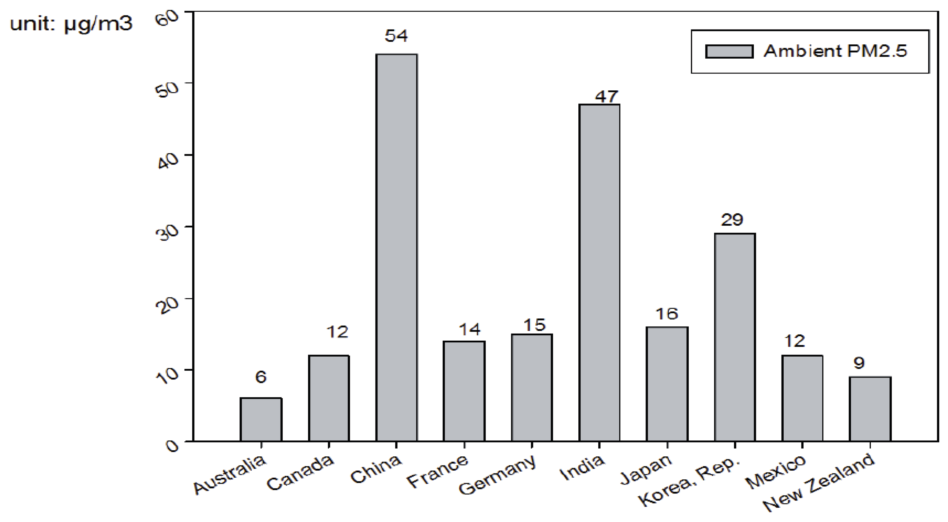
:1. Introduction
2. Methods and Data
2.1. The Direct Air Pollution Rebound Effect
2.2. The Elasticity Model
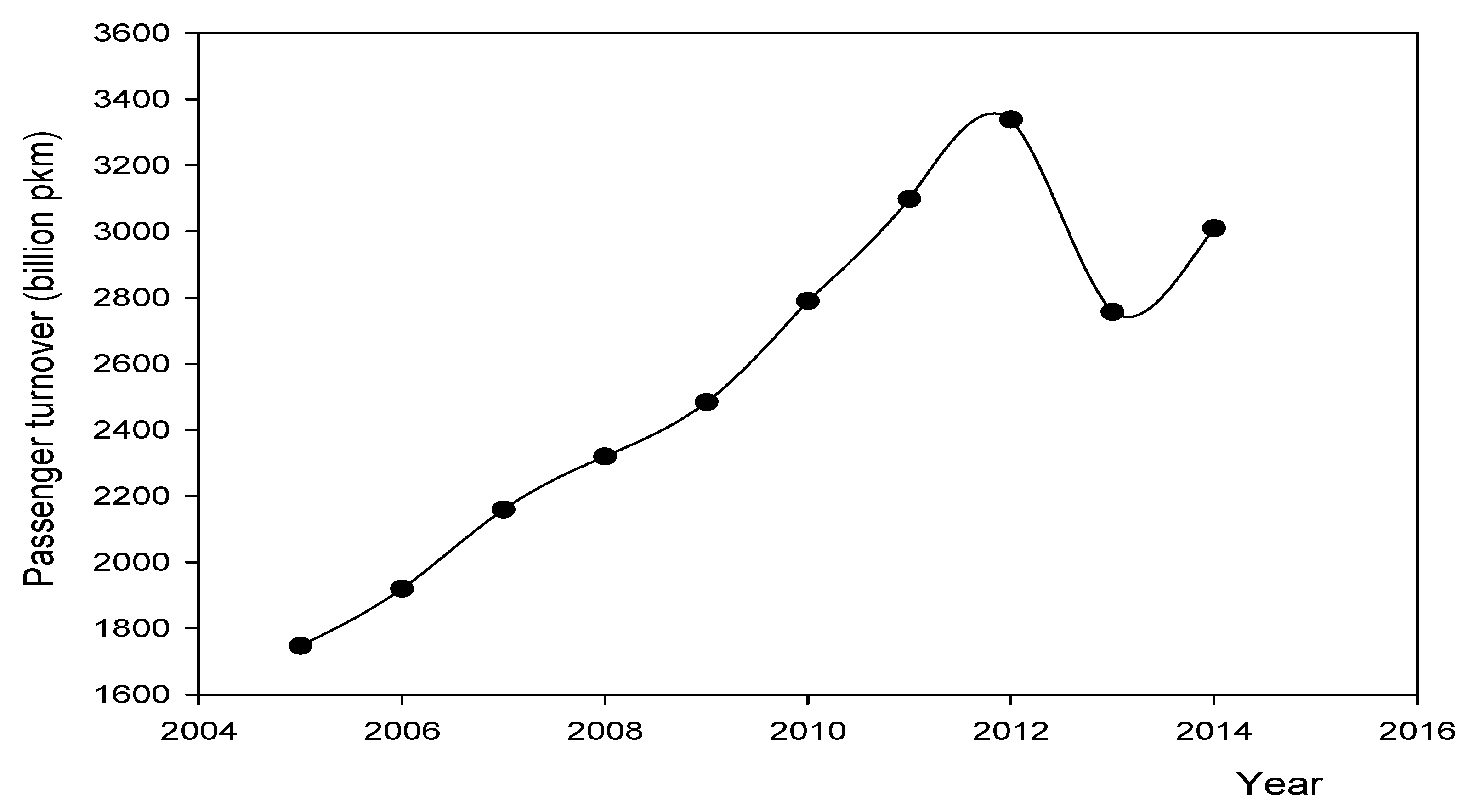
2.3. Data
3. Empirical Results and Discussions
3.1. Unit Root Test and Cointegration Test
3.2. Rebound Effect Estimation
4. Conclusions
Acknowledgments
Author Contributions
Conflicts of Interest
References
- World Bank. World Development Indicators 2007; World Bank: Washington, DC, USA, 2007; Available online: http://siteresources.worldbank.org/DATASTATISTICS/Resources/table3_13.pdf (accessed on 12 March 2017).
- World Bank. World Development Indicators 2016; World Bank: Washington, DC, USA, 2016. [Google Scholar]
- Ministry of Environmental Protection of the People’s Republic of China. The State of Environment (SOE) Report of 2016. Available online: http://www.mep.gov.cn/gkml/hbb/qt/201604/t20160421_335390.htm (accessed on 12 March 2017).
- Kunzli, N.; Kaiser, R.; Medina, S.; Studnicka, M.; Chanel, O.; Filliger, P.; Herry, M.; Horak, F.; Puybonnieux-Texier, V.; Quenel, P.; et al. Public-health impact of outdoor and traffic-related air pollution: An European assessment. Lancet 2000, 356, 795–801. [Google Scholar] [CrossRef]
- Hoek, G.; Brunekreef, B.; Goldbohm, S.; Fischer, P.; van den Brandt, P.A. Association between mortality and indicators of traffic-related air pollution in the Netherlands: A cohort study. Lancet 2002, 360, 1203–1209. [Google Scholar] [CrossRef]
- Samet, J.M. Traffic, air pollution, and health. Inhal. Toxicol. 2007, 19, 1021–1027. [Google Scholar] [CrossRef] [PubMed]
- Beelen, R.; Hoek, G.; van den Brandt, P.A.; Goldbohm, R.A.; Fischer, P.; Schouten, L.J.; Armstrong, B.; Brunekreef, B. Long-term exposure to traffic-related air pollution and lung cancer risk. Epidemiology 2008, 19, 702–710. [Google Scholar] [CrossRef] [PubMed]
- Weichenthal, S.; Kulka, R.; Dubeau, A.; Martin, C.; Wang, D.; Dales, R. Traffic related air pollution and acute changes in heart rate variability and respiratory function in urban cyclists. Environ. Health Perspect. 2011, 119, 1373. [Google Scholar] [CrossRef] [PubMed]
- He, L.Y.; Qiu, L.Y. Transport demand, harmful emissions, environment and health co-benefits in China. Energy Policy 2016, 97, 267–275. [Google Scholar] [CrossRef]
- Yang, G.H.; Wang, Y.; Zeng, Y.X.; Gao, G.F.; Liang, X.F.; Zhou, M.G.; Wan, X.; Yu, S.C.; Jiang, Y.H.; Naghavi, M.; et al. Rapid health transition in China, 1990–2010: findings from the global burden of disease study 2010. Lancet 2013, 381, 1987–2015. [Google Scholar] [CrossRef]
- Chen, S.M.; He, L.Y. Welfare loss of China’s air pollution: How to make personal vehicle transportation policy. China Econ. Rev. 2014, 31, 106–118. [Google Scholar] [CrossRef]
- Yang, S.; He, L.Y. Fuel demand, road transport pollution emissions and residents’ health losses in the transitional China. Transp. Res. Part D Transp. Environ. 2016, 42, 45–59. [Google Scholar] [CrossRef]
- He, L.Y.; Ou, J.J. Taxing sulphur dioxide emissions: A policy evaluation from public health perspective in China. Energy and Environment 2016, 27, 755–764. [Google Scholar]
- Ministry of Environmental Protection of the People’s Republic of China. China Vehicle Environmental Management Annual Report, 2016. Available online: http://www.mep.gov.cn/gkml/hbb/qt/201606/t20160602_353152.htm (accessed on 12 March 2017).
- National Bureau of Statistics of China. China Statistical Yearbook. Available online: http://www.stats.gov.cn/english/statisticaldata/AnnualData/ (accessed on 12 March 2017).
- He, L.Y.; Chen, Y. Thou shalt drive electric and hybrid vehicles: scenario analysis on energy saving and emission mitigation for road transportation sector in China. Transp. Policy 2013, 25, 30–40. [Google Scholar] [CrossRef]
- Liu, J.C. Energy saving potential and carbon emissions prediction for the transportation sector in China. Resour. Sci. 2011, 33, 640–646. [Google Scholar]
- Jevons, W.S. The Coal Question, 2nd ed.; Macmillan and Company: London, UK, 1866. [Google Scholar]
- Berkhout, P.H.; Muskens, J.C.; Velthuijsen, J.W. Defining the rebound effect. Energy Policy 2000, 28, 425–432. [Google Scholar] [CrossRef]
- Greening, L.A.; Greene, D.L.; Difiglio, C. Energy efficiency and consumption—The rebound effect—A survey. Energy Policy 2000, 28, 389–401. [Google Scholar] [CrossRef]
- Frondel, M.; Peters, J.; Vance, C. Identifying the rebound: Evidence from a German household panel. Energy J. 2008, 29, 145–163. [Google Scholar] [CrossRef]
- Sorrell, S.; Dimitropoulos, J. The rebound effect: Microeconomic definitions, limitations and extensions. Ecol. Econ. 2008, 65, 636–649. [Google Scholar] [CrossRef]
- Sorrell, S.; Dimitropoulos, J.; Sommerville, M. Empirical estimates of the direct rebound effect: A review. Energy Policy 2009, 37, 1356–1371. [Google Scholar] [CrossRef]
- Small, K.A.; Van Dender, K. Fuel efficiency and motor vehicle travel: the declining rebound effect. Energy J. 2007, 28, 25–51. [Google Scholar] [CrossRef]
- Barla, P.; Lamonde, B.; Miranda-Moreno, L.F.; Boucher, N. Traveled distance, stock and fuel efficiency of private vehicles in Canada: price elasticities and rebound effect. Transportation 2009, 36, 389–402. [Google Scholar] [CrossRef]
- Hymel, K.M.; Small, K.A. The rebound effect for automobile travel: asymmetric response to price changes and novel features of the 2000s. Energy Econ. 2015, 49, 93–103. [Google Scholar] [CrossRef]
- Wang, H.; Zhou, P.; Zhou, D.Q. An empirical study of direct rebound effect for passenger transport in urban China. Energy Econ. 2012, 34, 452–460. [Google Scholar] [CrossRef]
- Zhang, Y.J.; Peng, H.R.; Liu, Z.; Tan, W.P. Direct energy rebound effect for road passenger transport in China: A dynamic panel quantile regression approach. Energy Policy 2015, 87, 303–313. [Google Scholar] [CrossRef]
- Khazzoom, J.D. Economic implications of mandated efficiency in standards for household appliances. Energy J. 1980, 1, 21–40. [Google Scholar]
- Odeck, J.; Johansen, K. Elasticities of fuel and traffic demand and the direct rebound effects: An econometric estimation in the case of Norway. Transp. Res. Part A Policy Pract. 2016, 83, 1–13. [Google Scholar] [CrossRef]
- Alves, D.C.O.; da Silveira Bueno, R.D.L. Short-run, long-run and cross elasticities of gasoline demand in Brazil. Energy Econ. 2003, 25, 191–199. [Google Scholar] [CrossRef]
- Akinboade, O.A.; Ziramba, E.; Kumo, W.L. The demand for gasoline in South Africa: An empirical analysis using co-integration techniques. Energy Econ. 2008, 30, 3222–3229. [Google Scholar] [CrossRef]
- Sene, S.O. Estimating the demand for gasoline in developing countries: Senegal. Energy Econ. 2012, 34, 189–194. [Google Scholar] [CrossRef]
- Greene, D.L. Rebound 2007: Analysis of US light-duty vehicle travel statistics. Energy Policy 2012, 41, 14–28. [Google Scholar] [CrossRef]
- Editorial Department of Price Yearbook of China. Price Yearbook of China; Price Yearbook of China Press: Beijing, China, 1989–2015. [Google Scholar]
- National Bureau of Statistics of China. Price Statistical Yearbook of China; China Statistics Press: Beijing, China, 1988–1989.
- Hymel, K.M.; Small, K.A.; van Dender, K. Induced demand and rebound effects in road transport. Transp. Res. Part B Methodol. 2010, 44, 1220–1241. [Google Scholar] [CrossRef]


| Size | Existence | Policy Implication |
|---|---|---|
| PRE > 1 | Yes | Negative effect |
| PRE = 1 | Yes | Completely ineffective |
| 0 < PRE < 1 | Yes | Partially ineffective |
| PRE = 0 | No | Fully effective |
| PRE < 0 | No | Positive effect |
| Variable | lnVKM | lnY | lnP | lnV |
|---|---|---|---|---|
| Minimum | 2.2656 | 2.7330 | 3.0336 | 4.9571 |
| Maximum | 3.1348 | 4.3126 | 3.9354 | 6.6426 |
| Mean | 2.7032 | 3.5524 | 3.4951 | 5.6985 |
| Std. Dev. | 0.2558 | 0.4790 | 0.2901 | 0.5849 |
| Skewness | −0.1121 | −0.1432 | 0.0843 | 0.0350 |
| Kurtosis | 1.8700 | 1.9057 | 1.8197 | 1.3909 |
| Observations | 29 | 29 | 29 | 29 |
| Variable | DF Test | 1% Critical Value | 5% Critical Value | 10% Critical Value |
| −1.576 | −3.730 | −2.992 | −2.626 | |
| −0.681 | −3.730 | −2.992 | −2.626 | |
| −0.994 | −3.730 | −2.992 | −2.626 | |
| −1.293 | −3.730 | −2.992 | −2.626 | |
| −5.190 *** | −3.736 | −2.994 | −2.628 | |
| −5.545 *** | −3.736 | −2.994 | −2.628 | |
| −2.800 * | −3.736 | −2.994 | −2.628 | |
| −4.117 *** | −3.736 | −2.994 | −2.628 | |
| Variable | PP Test | 1% Critical Value | 5% Critical Value | 10% Critical Value |
| −1.643 | −3.730 | −2.992 | −2.626 | |
| −0.667 | −3.730 | −2.992 | −2.626 | |
| −0.791 | −3.730 | −2.992 | −2.626 | |
| −1.376 | −3.730 | −2.992 | −2.626 | |
| −5.193 *** | −3.736 | −2.994 | −2.628 | |
| −5.611 *** | −3.736 | −2.994 | −2.628 | |
| −2.919 * | −3.736 | −2.994 | −2.628 | |
| −4.117 *** | −3.736 | −2.994 | −2.628 |
| Rank | LL | Trace Statistic | 5% Critical Value | Max Statistic | 5% Critical Value |
|---|---|---|---|---|---|
| 0 | 192.45 | 64.93 | 54.64 | 36.37 | 30.33 |
| 1 | 210.64 | 28.56 | 34.55 | 16.23 | 23.78 |
| 2 | 218.75 | 12.33 | 18.17 | 7.95 | 16.87 |
| 3 | 224.92 | 4.38 | 3.74 | 4.38 | 3.74 |
| Dependent Variable | ||||
|---|---|---|---|---|
| Explanatory Variables | Coefficient | SE | t-Statistic | p Value |
| 0.4105 | 0.1793 | 2.29 | 0.032 ** | |
| 0.6023 | 0.2119 | 2.84 | 0.009 *** | |
| 0.0644 | 0.0248 | 2.60 | 0.016 ** | |
| −0.6690 | 0.3462 | −1.93 | 0.066 * | |
| 0.5375 | 0.3074 | 1.75 | 0.094 * | |
| Adjusted R-squared | 0.96 |
© 2017 by the authors. Licensee MDPI, Basel, Switzerland. This article is an open access article distributed under the terms and conditions of the Creative Commons Attribution (CC BY) license ( http://creativecommons.org/licenses/by/4.0/).
Share and Cite
Qiu, L.-Y.; He, L.-Y. Are Chinese Green Transport Policies Effective? A New Perspective from Direct Pollution Rebound Effect, and Empirical Evidence From the Road Transport Sector. Sustainability 2017, 9, 429. https://doi.org/10.3390/su9030429
Qiu L-Y, He L-Y. Are Chinese Green Transport Policies Effective? A New Perspective from Direct Pollution Rebound Effect, and Empirical Evidence From the Road Transport Sector. Sustainability. 2017; 9(3):429. https://doi.org/10.3390/su9030429
Chicago/Turabian StyleQiu, Lu-Yi, and Ling-Yun He. 2017. "Are Chinese Green Transport Policies Effective? A New Perspective from Direct Pollution Rebound Effect, and Empirical Evidence From the Road Transport Sector" Sustainability 9, no. 3: 429. https://doi.org/10.3390/su9030429