
Numerical Modeling and 3D Investigation of INWAVE Device


1
Department of Electrical and Electronic Engineering, Yonsei University, 50 Yonsei-ro, Seodaemun-gu, Seoul 03722, Korea
2
INGINE Inc., Changdo Building, 395-2 Cheonho-daero, Dongdaemun-Gu, Seoul 03722, Korea
*
Author to whom correspondence should be addressed.
Sustainability 2017, 9(4), 523; https://doi.org/10.3390/su9040523
Submission received: 18 February 2017
/
Revised: 25 March 2017
/
Accepted: 27 March 2017
/
Published: 30 March 2017
(This article belongs to the Special Issue Wave Energy Converters)
Abstract
:In this article, numerical studies on a tightly moored point absorber type wave energy converter called INWAVE are presented. This system consists of a buoy, subsea pulleys, and a power take off (PTO) module. The buoy is moored by three ropes that pass through the subsea pulleys to the PTO module. Owing to the counterweight in the PTO module, a constant tension, which provides a horizontal restoring force to the buoy, is constantly applied to the rope. As waves pass by, the buoy is subjected to six degrees of freedom motion, consisting of surge, heave, sway, roll, pitch, and yaw, which causes reciprocating motion in the three mooring ropes. The PTO module converts the motion of the ropes into electric power. This process is expressed as a dynamic equation based on Newtonian mechanics and the performance of the device is analyzed using time domain simulation. We introduce the concept of virtual torsion spring in order to prevent the impact error in the ratchet gear modules which convert bidirectional motion of rope drum into unidirectional rotary motion. The three-dimensional geometrical relationship between the ropes and the buoy is investigated, and the effects of the angle of the mooring rope and the direction of wave propagation are addressed to determine the interaction between the tension of the rope and the buoy. Results have shown that the mooring rope angle has a large impact on the power extraction. The simulation results present a useful starting point for future experimental work.
1. Introduction
Ocean wave energy is a renewable energy source with high energy density and great potential. Ocean waves have higher energy density as they are deeper offshore. The water particles here draw a circular orbital trajectory. Conversely, and the lower the depth of water, the closer the ocean is, the lower the energy density of the waves, and the water particles have the orbitals of long transverse orbits. That is, as the water depth decreases, the energy distribution in the horizontal direction becomes larger. In the shallow sea, furthermore, the irregularity of the waves becomes larger depending on the terrain of the sea floor [1,2].
Depending on the characteristics of the waves due to these water depths, the power generation mechanism from waves varies greatly depending on the place where the wave energy converter (WEC) is installed [3,4]. It is advantageous to use the heave motion in the deep sea, and point absorber types such as OPT PowerBuoy [5], Wavebob [6], and CETO [7] have been studied to maximize vertical energy absorption. The attenuator-types WEC resembling the inverted oscillator such as Oyster [8,9] and WaveRoller [10] are advantageous for absorbing energy mainly in the surge direction. It is therefore suitable for areas with lower depths than the target area of the point absorber. The coastal installation of WEC is led by the fixed-structure oscillating water column (OWC) types that were built in Norway (in Toftestallen, near Bergen, 1985, [3]), Japan (Sakata, 1990, [11,12]), India (Vizhinjam, near Trivandrum, Kerala state, 1990, [13]), Portugal (Pico, Azores, 1999, [14]), UK (the LIMPET plant in Islay Island, Scotland, 2000, [15]), Spain (breakwater OWC, Mutriku, Northern Spain, 2008, [16]), and Italy (U-OWC, Civitavecchia, 2012 [17,18]). Recently, moving from the experience of the offshore over-topping devices (OTD) Wavedragon [19] and the Sea-wave Slot-cone Generator [20], an onshore OTD has been built in Italy [21]. Fixed-structure OWCs and OTDs have good accessibility and maintainability, but there are topographical constraints where the wave energy density should be high and the civil construction should be possible.
The distinction by such depth or distance from the land determines the motion mechanism. In addition, the more distant the sea, the higher the cost of the facilities required for electric transmission to areas where electricity is mainly consumed. There is another alternative to electric transmission. The CETO and Oyster WECs pump the seawater to the land that drives the generator, so the sea water pipe replaces the electric transmission cable. In this case, it is very advantageous for maintenance of the generator since the generator is located on the land. That is, the way to transfer energy to the land is also a main factor in determining the mechanism of wave power generation.
Meanwhile, one of the areas where the introduction of wave power is difficult is the area where the water depth is shallow and wave irregularity is large. In this area, it is difficult to design the mechanism of conversion process from wave to mechanical energy; however, accessibility on land is comparatively good, and it is distributed all over the world. There is a need for a WEC capable of targeting these areas. It is expected that such areas will need a strategy of securing the desired capacity by installing multiple WECs with small capacity rather than a single large capacity WEC, and the cost of a single device should be cheap.
The off-grid islands have a great need for the development of these wave devices, where there is no power supply from the mainland. According to reports from the Korea Electric Power Corporation (KEPCO), electric power costs in these areas are eight times higher than those on the land [22]. In many of these areas, the required amount of electric power is often small, such as several tens of kilowatts. Therefore, a small capacity wave generator is more suitable for these areas.
The wave power company INGINE has created a wave power generator called INWAVE, which is a wave generator suitable for coasts with shallow water depths and wave irregularities [23]. This is a multi-tight moored moving object, sharing similar concepts with Fred Olsen’s Lifesaver WEC [24]. However, unlike Lifesaver, INWAVE has a reinforced mechanism to cope with the wave force in a horizontal direction as the installation depth is low. It is also advantageous for maintenance because the PTO module is located on the coast.
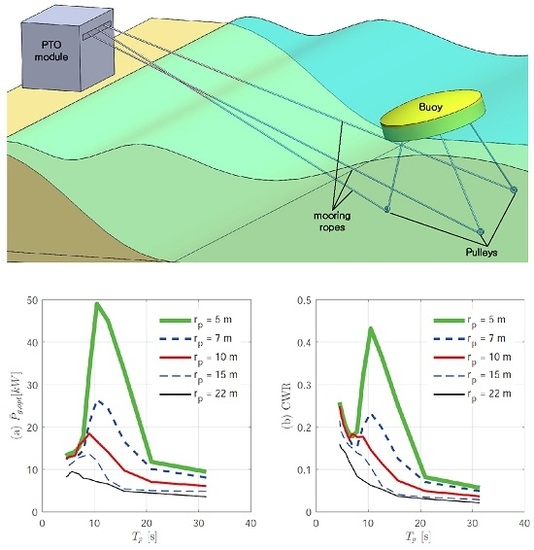
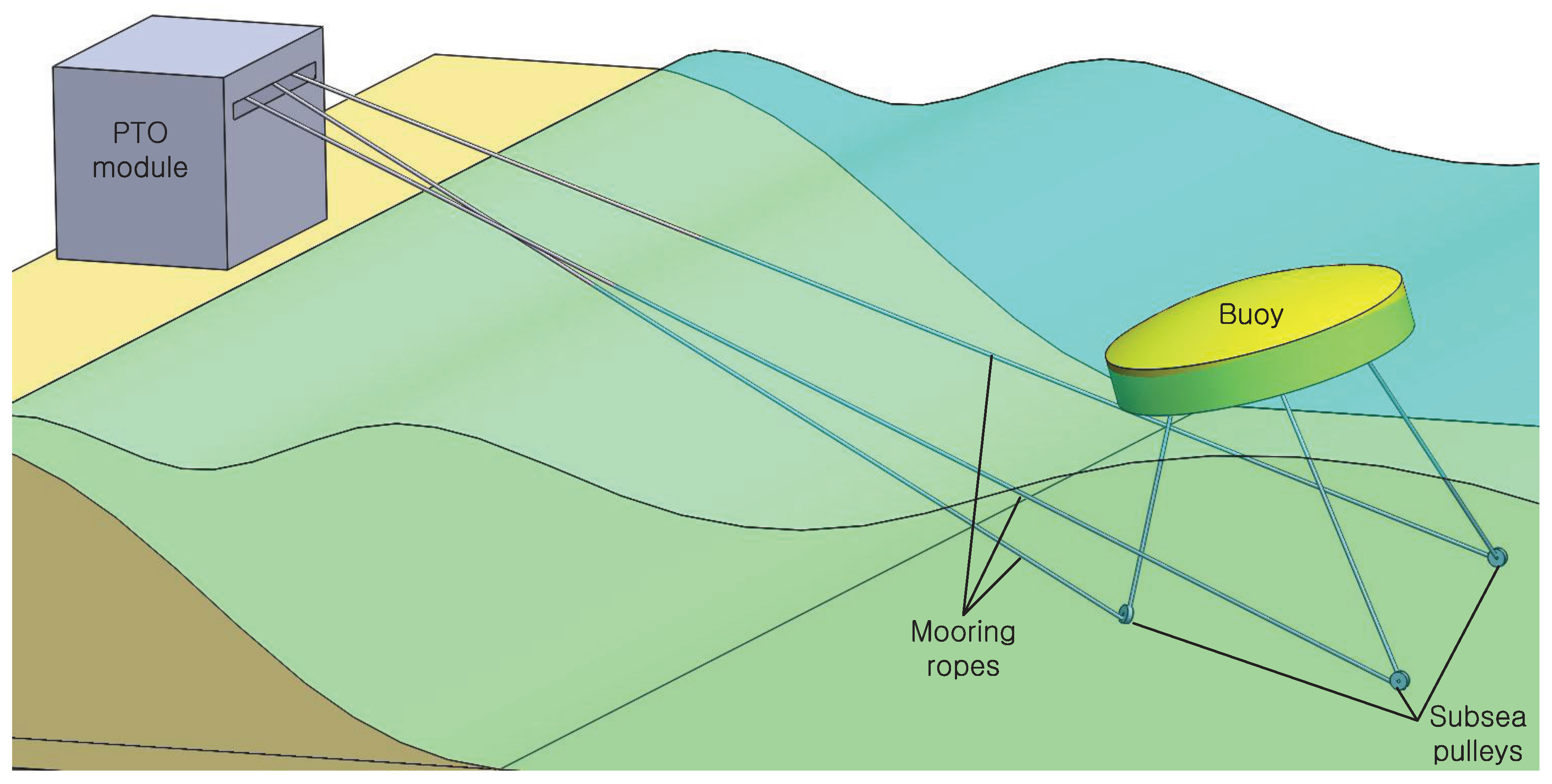
It mainly consists of a buoy, subsea pulleys, and a power take off (PTO) module as shown in Figure 1. Three mooring ropes are attached to three points on the bottom of the buoy and also connected to three counterweights in the PTO module via subsea pulleys on the sea-bed. The counterweight moves only vertically and this provides restoring force to the buoy, and the buoy performs six degrees of freedom movement of heave, surge, sway, roll, pitch, and yaw within a certain range. In addition, the tension prevents the rope from sagging and serves to transfer the kinetic energy of the buoy to the PTO module. As the buoy moves, the three ropes reciprocate and also the rope pulleys in the PTO module that rotate back and forth share one shaft and transmit unidirectional rotary motion to the common shaft through their ratchet gears. This rotational energy is then converted into electrical energy by the electric generator. When the buoy is pulling the rope, the tension of the rope raises the counterweight while transmitting power to the common shaft through the ratchet gear. On the other hand, when the buoy is no longer pulling the rope, the tension is provided by the counterweight, which pulls the buoy back to its equilibrium position. However, during this time, the ratchet gear cuts off the work of the counterweight, so there is no power transmitted to the common shaft.
The two-dimensional modeling and simulation of INWAVE has been presented in a previous paper [25]. This modeling assumes that only two ropes are connected between the buoy and the PTO module unlike the actual plant, and only surge, heave, and pitch motions of the buoy were considered while sway, roll, and yaw motions were ignored as a limitation of the two-dimensional analysis. In this paper, a three-dimensional model of the INWAVE device is presented, which considers the six degree motion of the buoy and the three mooring rope’s connections in order to overcome previous assumptions. To build this dynamic model, the geometric relationship between the behavior of the buoy and the ropes in the three-dimensional space was identified, and, based on this, we derived the overall dynamics by combining the hydrodynamic coefficients for the buoy using an ANSYS AQWA simulator [26] and the PTO module based on the Newtonian mechanics and linear wave theory (LWT) [27,28]. Next, we carried out simulations under regular wave conditions with varying wave periods to analyze the effects of the mooring rope angle, counterweight’s mass, and wave incidence angle, which are the most important factors that influence the system output. Then, for objective efficiency comparison with other WECs, we analyzed the theoretical performance of the device by calculating the capture width ratio (CWR) that is the average power output of the device divided by wave energy density and the diameter of the buoy under irregular wave conditions based on the joint north sea wave project (JONSWAP) wave spectrum model.
2. Geometrical Relationship between Buoy and Ropes in Three-Dimensional Space
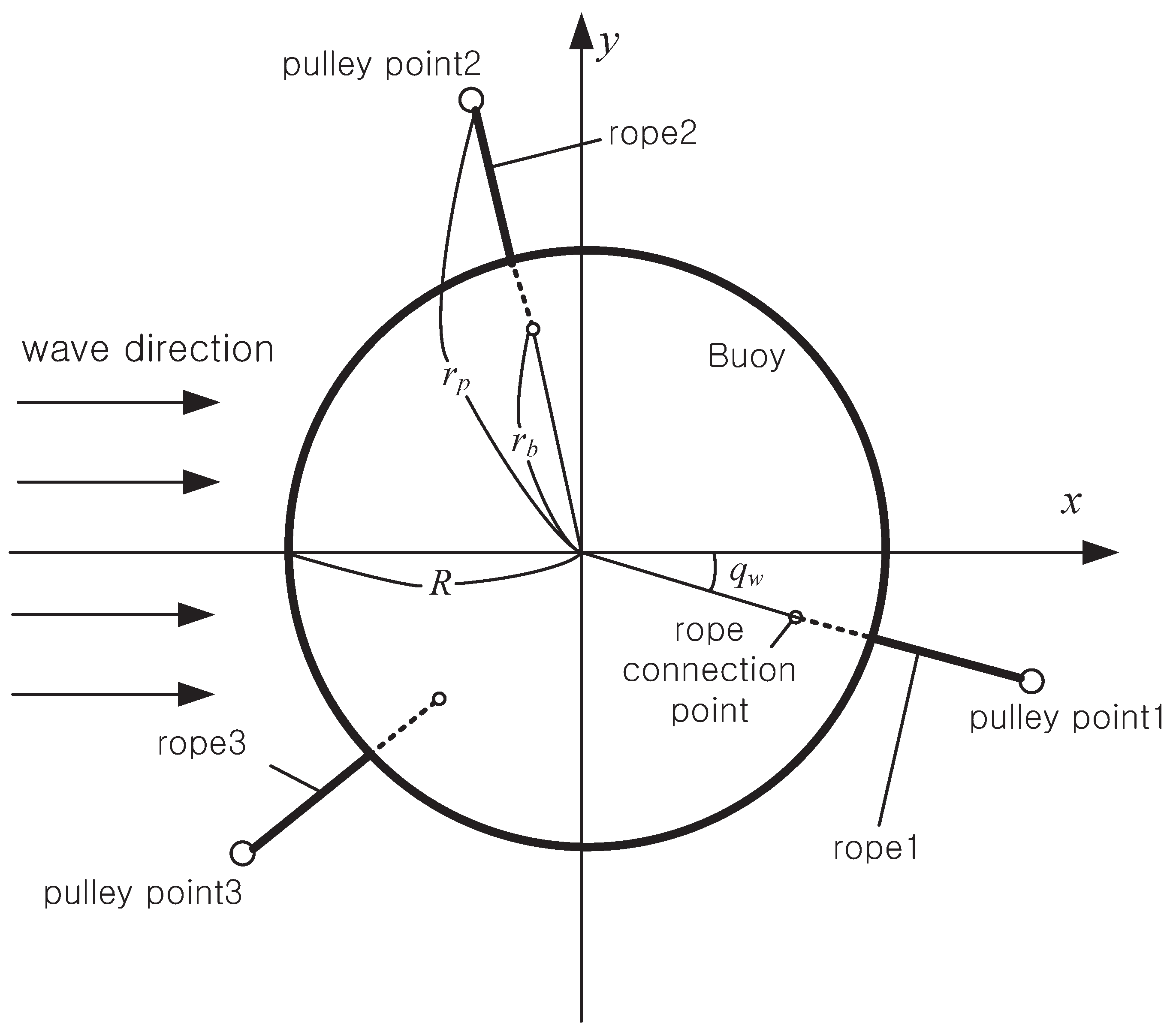
Consider a buoy in the sea with a depth of h, where the buoy radius and draft are R and d, respectively. The behavior of the buoy is given by corresponding to surge (x), sway (y), heave (z), roll (), pitch (), and yaw (), respectively, since the wave propagates in the x-direction. The top view of the buoy, subsea pulleys, and rope connection points are shown in Figure 2. An actual device is installed near the breakwater. Unfortunately, ANSYS AQWA, which is a computational fluid dynamics simulator to obtain the hydrodynamics, assumes a flat undersea surface and does not provide an effect on reflected waves. Hence, it is assumed that the buoy is installed on open sea.
At the bottom of the buoy, the ropes are connected at a distance of , and the connection points make an angle of 120 with each other. At the bottom surface of the sea, the three subsea pulleys are each located at a distance of from the center and are arranged at an angle of 120 with respect to each other.
In the equilibrium state, since the forces exerted on the buoy are only the tensions of the ropes exerted by the counterweight and buoyancy in the heave direction, the center of the subsea pulley and the buoy are placed on the z-line, and each pulley and rope connection point are placed on the same line from the center. Since the buoy is z-axis symmetry, the direction of wave propagation only affects the the rope connection points. Hence it is assumed that the wave direction is heading to the x-direction as seen in Figure 2 and the relative angle between the wave direction and the rear pulley is defined as , which has a value of –60 to 60, but is limited to a range of 0 to 60 by symmetry.
The dynamic model of the device includes the influence of the rope tensions; hence, the geometric analysis between the rope connection point and subsea pulley is necessary. First, the positions of rope connection points and the subsea pulleys must be defined in three dimensions. For convenience, let the position of ith rope connection point and subsea pulley point be and , respectively. These points can be derived using the homogeneous transformation matrices and as follows [29]:
where , , , and are defined as
and are the last column vectors of and that can be expressed as follows:
where (for i = 1, 2, 3). From this relationship, the ith rope vector is given by
The ith length of the rope , the speed of the rope (or ), and the acceleration of the rope (or ) are expressed as follows:
3. Dynamics of the Buoy and Rope Tension
The equations of buoy motion in surge, sway, heave, roll, pitch, and yaw directions can be expressed in Newtonian mechanics based on the LWT [27,28]. These six equations representing each axis are influenced by the excitation force due to waves, radiation damping caused by buoy motion, buoyancy, and rope tensions. The six equations are expressed as one vector equation that can be expressed as [25,27]:
Here, is the mass matrix consisting of buoy mass, buoy inertia, and added mass, is the radiation damping force vector, and is the buoyancy spring coefficient matrix. is the ith matrix of the rope tension effect on the buoy and is the tension applied to the ith rope. is the excitation force vector. can be expressed as
where ⊗ represents a cross product.
and are given as [25]
where , , , and represent the buoy’s masses and inertia of the x-, y-, and z-axes, respectively. Furthermore, , , , , , and are the added masses and inertia at infinity for the buoy’s surge, sway, heave, roll, pitch, and yaw motions, respectively.
and g denote the sea water density and the gravitational acceleration, respectively. is a diagonal matrix.
As described above, the wave direction is limited to the x-direction and it yields the excitation forces of surge, heave, and pitch, only acting on the buoy due to the buoy’s symmetry, and other components are omitted. The excitation force vector can be computed as a convolution of the water surface elevation and impulse response function from the frequency domain results. denotes the time shift for convolution:
where , , and denote the excitation kernel functions for surge, heave, and pitch, respectively, which can be obtained by the following formula:
where is the excitation force in the frequency domain and is the phase shift of the excitation force, which is , 0, and for surge, heave, and pitch, respectively. This phase shift is necessary for the same reason that water particles by the waves cause the orbital motion [1].
Similarly, the radiation damping force, which is a resistance component, can be obtained by convolution of the buoy’s velocity and radiation kernel function as follows [30]:
where
Here, , and and denote radiation damping and added mass in the frequency domain, respectively. It is assumed that there is no resistance in the yaw direction because this part is disk-shaped.
4. PTO Modeling
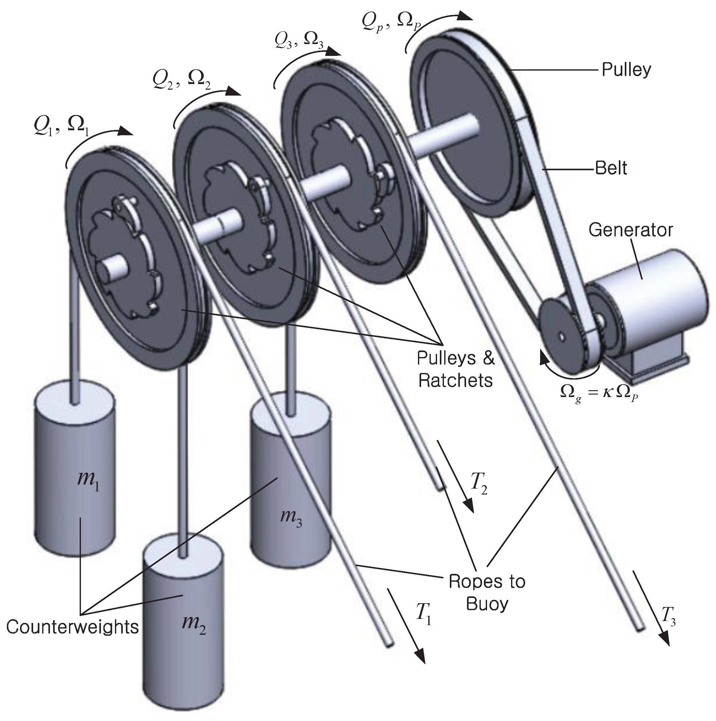
Figure 3 is a simplified representation of the configuration of the PTO module. In the PTO module, three mooring ropes hang on rope pulleys and three counterweights are attached to the end of the ropes to provide constant tension equal to their weight. The rope pulley has a ratchet gear module that only transmits torque to the common shaft when the rope is pulled by the buoy. The rotation of this shaft is increased by the gear ratio and transmitted to the generator. The angle and angular velocity of the ith rope pulley are and , respectively, while that of the common shaft and generator are and , and and , respectively. Then, these variables have the following relationship:
where is the ith pulley radius. Assuming that there is no inertia of the shaft and pulleys, the dynamics of the generator are given as follows:
where is the generator inertia, is the torque transmitted by the ith pulley, and is the induced torque applied by the generator and is given as
where is the generator damping coefficient that can be controlled using an inverter at the rear end of the generator. The instantaneous output from the generator is defined as
The ratchet gears continuously supply and block the torque from the rope pulley to the common shaft. When the torque is transmitted, the rope pulley and the common shaft are coupled and driven as one part, and when the torque is not transmitted, the two parts move independently. At the moment when the rope pulley and the common shaft are combined, the analysis is linked to their physical properties such as the strength and elastic modulus and is difficult to model using Newtonian mechanics. Therefore, to solve this problem, we introduced a virtual spring concept in the ratchet module in our previous paper [25]. This spring occurs at the moment of contact between the pulley and the common shaft, momentarily stores the compressed force as potential energy, and gradually transfers this energy to the shaft without power loss. Then, as soon as negative torque is transmitted through the spring, the pulley and the common shaft are separated. This process can be expressed as follows:
where is the spring coefficient of the virtual spring, and is the time of contact (). Then, when , the contact between the ratchet and the shaft is released.
The dynamic equation of the counterweight, including the transmitted torque to the shaft, is as follows:
The power transfer efficiency of the ratchet gear to the generator during one wave peak period is defined as follows:
5. Simulation and Analysis under Regular Wave Condition
Currently, a prototype installed on Jeju Island has a buoy diameter of 5 m and the maximum power is obtained in a period between 2.5 and 4.5 s [25]. However, the wave period of the area under consideration for installation is 7 to 12 s. By the simulation of buoys with various geometries, it was found that a diameter of 12 m is suitable for the target area. Therefore, in this paper, a simulation is performed based on a buoy with a diameter of and a draft of .
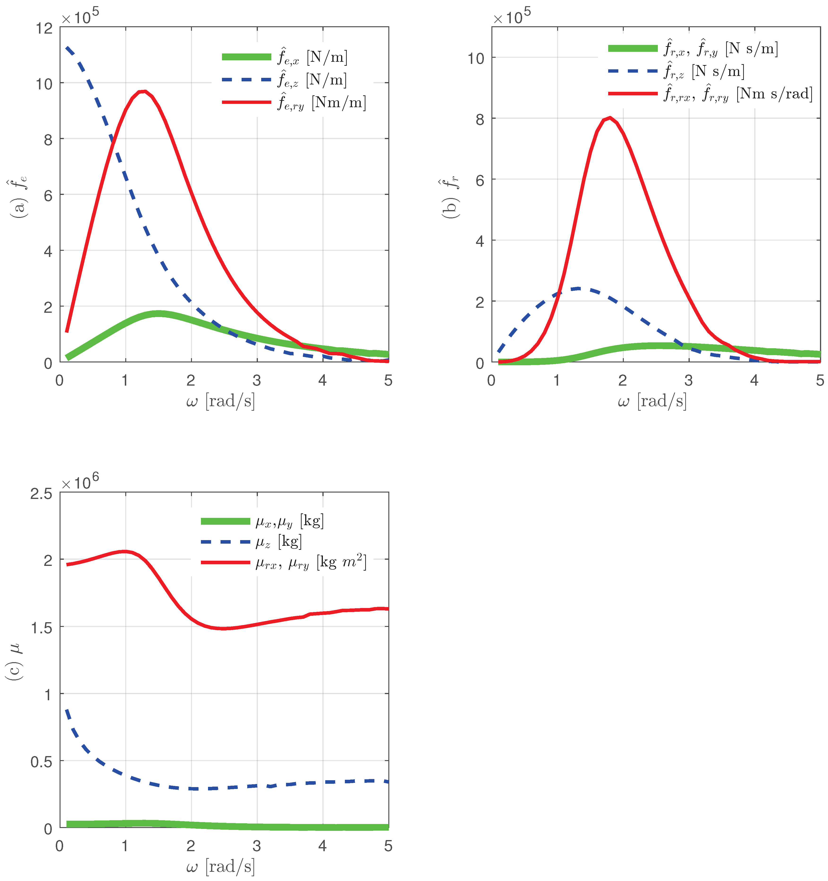
In order to perform simulation on the WEC system, we need the hydrodynamic data such as excitation force, radiation damping, and added mass in the frequency domain. The ANSYS AQWA simulator was used to obtain the data [26]. A disk-shaped buoy with a diameter of and a draft of was applied floating on a sea with a depth (h) of 10 m; the acquired data are shown in Figure 4. This simulator is based on LWT and assumes incompressible, irrotational flow with small amplitude motion [27,28]. Therefore, the simulation only considers the case of 1 m wave height ().
By substituting this data into Equations (21) and (23), we obtain the kernel functions, and then substituting the wave elevation and the excitation kernel function into Equation (20) yields the excitation force in the time domain. As mentioned in the previous section, the overall dynamic equation consisting of Equation (32) with Equations (26) and (29) is analyzed in the time domain using the fourth-order Runge–Kutta method [31].
In the modeling of INWAVE, the influence of the rope is included in . Since this matrix has nonlinearities including the trigonometric function, the analysis of the overall modeling is impossible in the frequency domain. Therefore, the simulation under the regular wave condition in the time domain was carried out to analyze the exact dynamic behavior of the device with the characteristics of the power output. The following sine wave was generated for regular wave condition:
where and are the significant wave height and peak wave frequency, respectively.
The output power of the WEC is sensitive to generator damping load . We substitute between and , and denote when the average of the maximum output power from generator is obtained. The data for all parameters required to perform the simulation are listed in Table 1. In order to observe the characteristics of each wave frequency, was fixed at 1 m and was assigned at intervals of 0.1 rad/s between 0.2 and 1.4 rad/s. The total sampling time was where , and only the results within to were recorded in order to exclude the data in the transient segment. Except for defined in Equation (31), the mean value () and standard deviation () used the data in this interval.
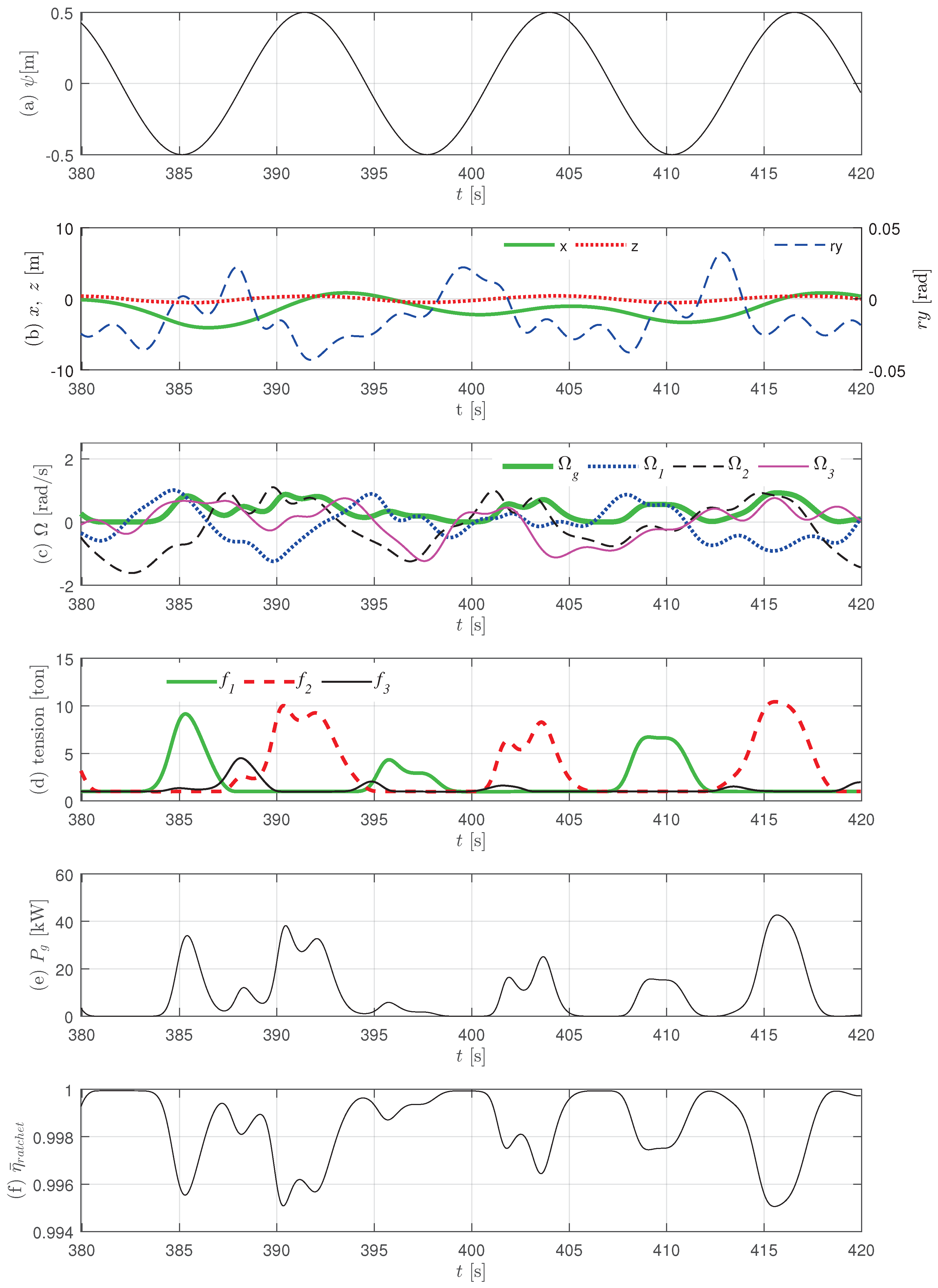
The INWAVE device has all the states intertwined because the buoy moves in six degrees of freedom and three ropes are connected to the single generator. Therefore, it is hard to obtain the perfect periodicity of the states according to the wave period even in regular wave conditions. In the case of , , Nm·s/rad, 30, and () as presented in Table 1, while the simulation results are shown in Figure 5. Figure 5b shows that the surge, heave, and pitch motions of the buoy have periodicity with the wave period and out of these parameters, the surge has the highest amplitude. In Figure 5c–e, however, the angular speeds of the rope pulley and generator, rope tensions, and power output do not have repeated patterns. In Figure 5c, the angular velocity of the generator follows the highest value of the angular velocity of the rope drum, but not perfectly. Even then, the average efficiency of the ratchet in Figure 5f is approximately 1. Accordingly, it can be estimated that there is no power loss in the ratchet transmission. The rope tension in Figure 5d only increases when the power is transferred; otherwise, it acts on the rope only as much as the counterweight’s mass.
As can be seen in Figure 5, the device has a strong nonlinearity and cannot be directly analyzed in the frequency domain. Therefore, we resolved to understand the behavior and performance of the device by taking the average data for a long period of time in the time domain while varying several parameters such as the pulley position , mass of the counterweight , and the wave direction .
5.1. Influence of Subsea Pulley Position
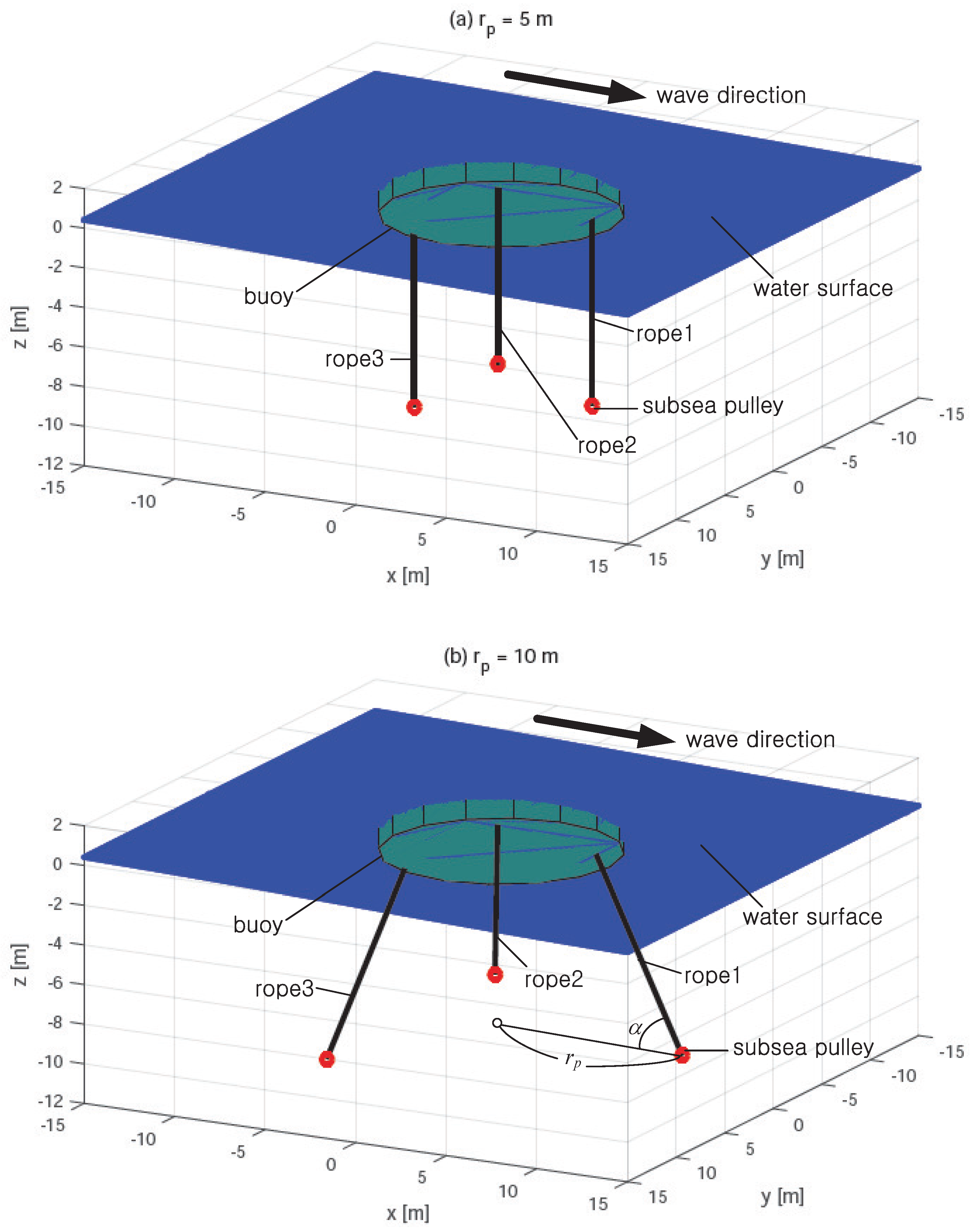
The simulation was carried out where the rope connection points at the bottom of the buoy were fixed at and the position of the subsea pulley was selected from 5, 7, 10, 15, and 22 . The mooring rope’s angle corresponding to with the sea floor is given in Table 2 and Figure 6 shows the rendered image of the buoy and ropes with according to . In the case of , the rope tension acts on the buoy only in the vertical direction, and as increased, the horizontal component of the rope tension acting on the buoy also increased.
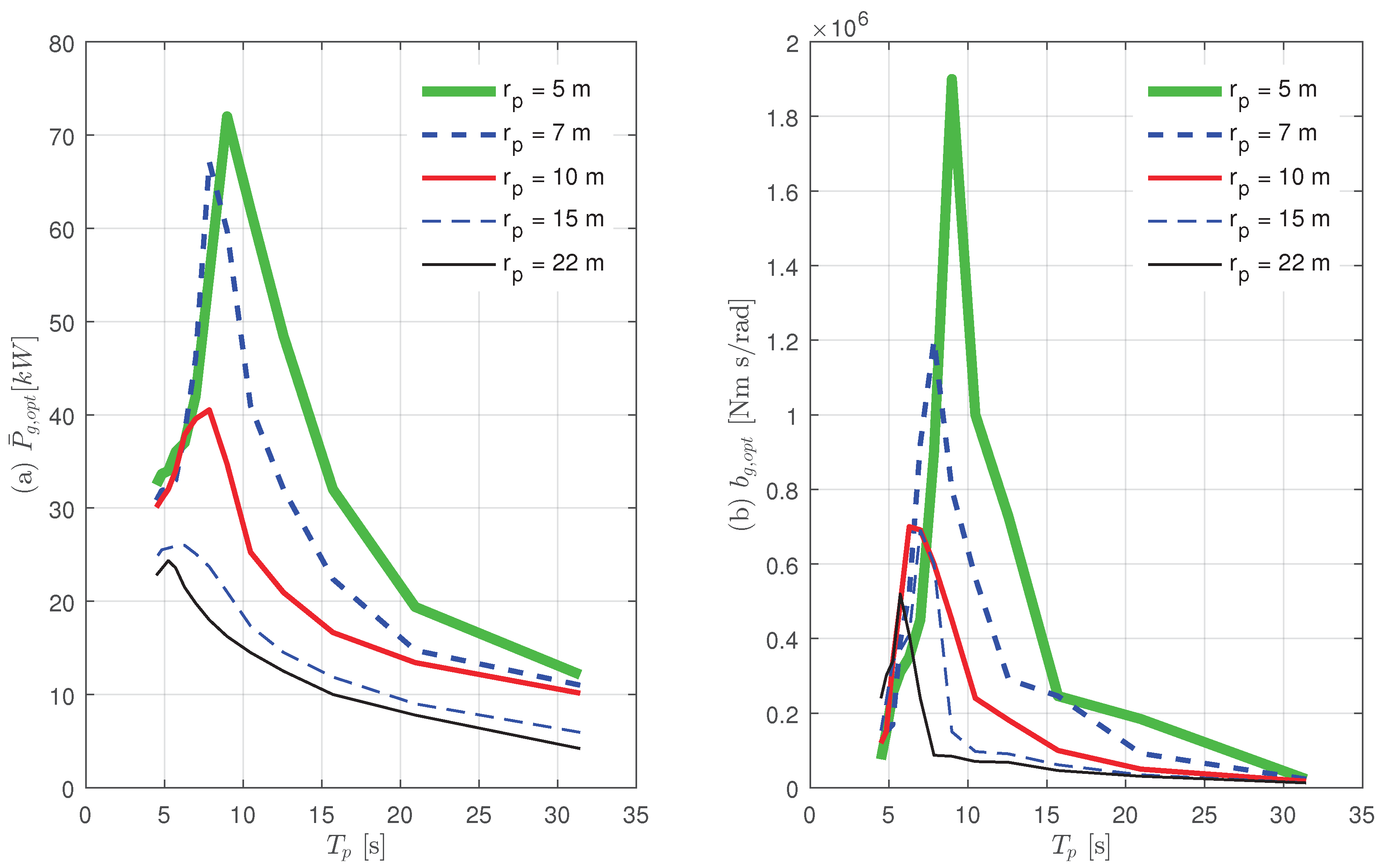
Figure 7 shows simulation results of the average maximum power output and the corresponding damping load at various values that can be obtained at each wave period. In the graph, the case of showed the highest average power and the power decreased as increased. In addition, it can be seen that the wave period of the peak power output slightly decreased while the increased. The smaller the , the larger the lateral force tension generated, which affects the resonance period. also influences how efficiently the movement of the buoy is transmitted to the displacement of the rope. As the rope connection point moved in the tangential direction around the subsea pulley, the change in the length of the rope decreased, so that the transmission rate of the kinetic energy was reduced. Therefore, we define a rope kinematic efficiency factor in order to determine the effectiveness of transmitting the buoy’s motion to the rope’s displacement, which can be defined by the ratio of the absolute value of the rope connection point speed to the speed of the rope length. This can be expressed as follows:
As the efficiency was very close to 1, the movement of the rope connection point was effectively transmitted to the change in the length of the rope.
For a more accurate analysis, we compared the power output, behavior of the buoy, and displacement of the rope for variations in values between 5 and 22 m as seen in Table 2 at 4.49, 8.98, and 12.57 s; the results are shown in Figure 8. Figure 8a shows the optimal mean power and Figure 8b–d show the normalized standard deviation in the direction of surge, heave and pitch, which denotes the standard deviation of the displacement divided by the amplitude of the wave. Figure 8e,f show of ropes 1 and 2, respectively. Since , the motion of rope 3 is the same as that of rope 2, and it is omitted. Figure 8g,h are the motion transfer efficiencies of the rope. First, let us consider the results for 7.85 and 15.71 s in order to analyze the concentration of power output in 7–15 s of the wave period.
In Figure 8a, the power output tends to decrease as increased and the result is similar to In Figure 8b, it can be seen that is overwhelmingly higher than and in Figure 8c,d, respectively. This means that the output of the device depends mostly on the surge movement. It seems to be a good choice to choose m in order to maximize the motion in the surge direction, but the opposite tendency can be seen from Figure 8e–h. In Figure 8e,f, when 15.71 s, it can be seen that increased with increasing until 15 m because the increasing rate of is higher than the decreasing rate of . The dynamic modeling so far considered did not take into account resistances other than radiation damping such as friction and viscosity. If all resistive components were considered, a large as shown in Figure 8b cannot be expected. Therefore, the actual model should select considering both the effects of surge displacement and the motion transfer efficiency of the rope. In addition, the case of 4.49 s is different from 15.71 and 7.85 s. It should be noted that Figure 8g,h, showed a very high near 5 m. This is because the pitching motion increased as decreased, which affects the normal direction movement of the rope rather than the surge and heave.
5.2. Influence of Counterweight
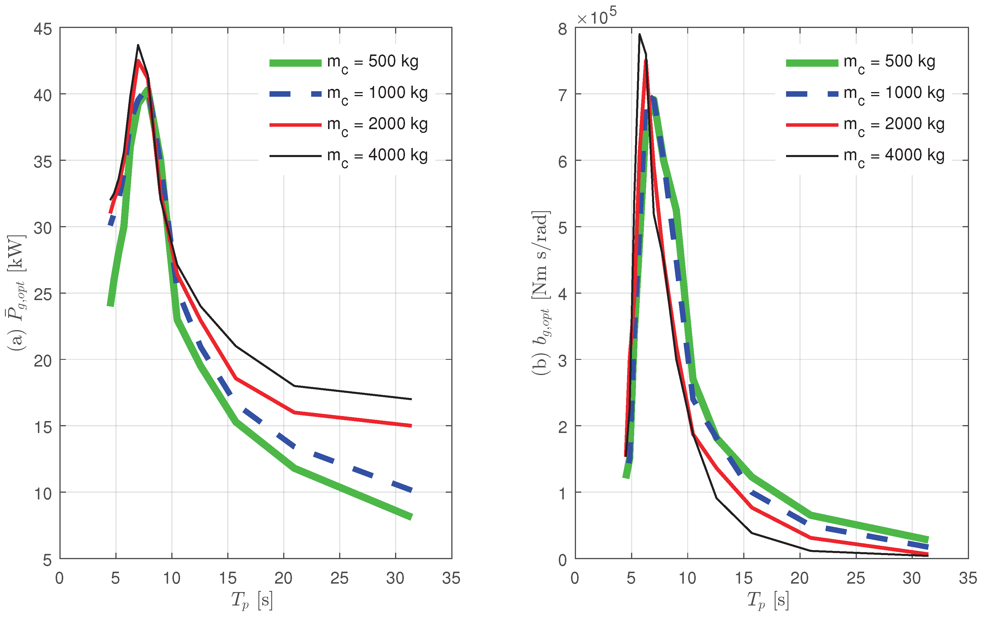
In order to evaluate the effect of the counterweight, we carried out a simulation for the case when 10 m was fixed and was set to 500, 1000, 2000, and 4000 kg. The other parameters remained the same as shown in Table 1. Figure 9 shows the maximum power output and the corresponding . As increased, generally increased, but the extent of the increase gradually decreases. The increase in the power output by the counterweight was prominent in the long period, and the effect was small in the short period. In addition, as increased, the peak of the output shifts slightly to the smaller period, but this tendency is not noticeable.
5.3. Influence of Wave Direction
In order to analyze the influence of the direction of the wave, the average power output and the standard deviation were calculated for various wave directions such as 10, 20, 30, 40, 50, when m, Nm·s/rad. Figure 10 shows the results of the power output with varying wave direction for 15.71, 7.85, and 4.49 s, where the thick green line is the average output and the red line is the standard deviation. When 15.71 s, the average power and standard deviation decreased slightly at approximately 20–30, although this is not significant. When 7.85 s, the average power and standard deviation increased by approximately 30% at 30. In the case of 4.49 s, the average output and standard deviation decrease by approximately 20% as the angle increased. Synthetically, consistent trends could not be derived, so we could not identify meaningful effects of the wave direction.
6. Simulation and Analysis under JONSWAP Irregular Wave Condition
In this section, let us compare the optimal average power for an irregular wave condition with the theoretical wave energy density. We chose the JONSWAP wave model because the target area where the INWAVE device has been installed has of the JONSWAP spectrum [32,33]. When the significant wave height is and the peak period is , it is expressed in the frequency domain with wave angular frequency as
where
The wave power per unit crest length is defined as
where
and
Here, the wave number ( is the wave length) is obtained from
When discussing the performance of many wave power systems, the availability and presentation of data vary greatly between sources. Therefore, many devices use a capture width ratio (CWR) to objectively compare the conversion efficiency. For a cylindrical buoy, the CWR is the average power output divided by and the diameter of the buoy and is expressed as [34]:
For time series calculations, the spectral distribution in Equation (35) is discretized as the sum of a large number N of regular waves and written as
Here, , where is the lowest frequency, is a small frequency interval, and the spectrum does not contain a significant amount of energy outside the frequency range . and are the amplitude of the wave component of order n and the initial phase randomly chosen in the interval , respectively. This wave elevation is substituted into Equation (20), and the simulation was carried out with the equivalent parameters in Table 1.
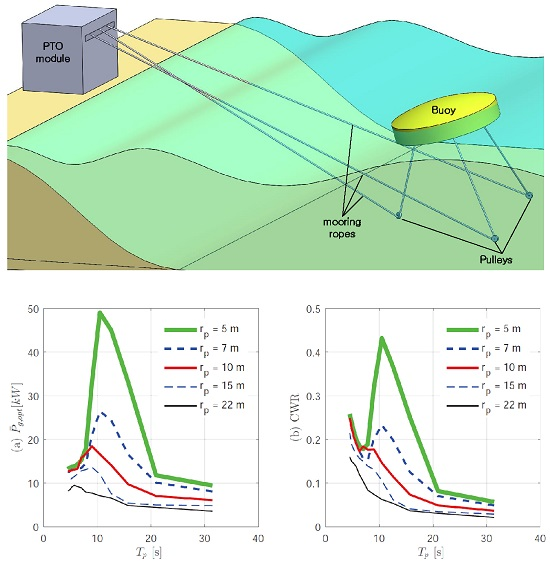
The average power output under irregular waves in Figure 11a was lower than that of the regular wave, but its pattern is similar to that of the regular wave. When 5 m, the highest power output was obtained and the output power gradually decreased as increased. The CWR shown in Figure 11 exhibited a similar pattern, having a peak of 0.43 at m, and the peak gradually disappeared as the increased. In addition, it can be seen that the CWR was much lower at a wider spectrum than in our previous paper [25]. This is a characteristic of the general point observer that can be seen as the diameter of the buoy increases.
Figure 12 shows the standard deviations of the buoy’s behavior in each direction, the standard deviation of the rope motion, and the motion transfer efficiency of the rope, which were also similar to that of the regular waves shown in Figure 8. At 15.71 and 7.85 s, the surge showed the greatest movement, and it decreased rapidly as decreased. In addition, the efficiency of the rope increased as increased, similar to the results of the regular wave condition.
7. Conclusions
In this study, we derived the three-dimensional dynamics of the INWAVE device and carried out simulations in time domain under regular and irregular wave conditions while varying various parameters such as the subsea pulley position, the counterweight’s mass, and the wave direction. The analysis of the results show that the distance between the subsea pulleys significantly affects the behavior of the buoy, the displacement of the rope, and the shape of the power output. The smaller the value of , that is, as the mooring angle approached 90, the dynamic behavior of the buoy became higher; however, the motion transfer efficiency of the rope decreased. This is because a large mooring angle leads to higher movements of the rope in the tangential direction, which decreases the effect on the rope length change. Since the dynamic behavior of the actual buoy motion would be greatly reduced by the unconsidered resistance factors, it may be better to consider the motion transfer efficiency of the rope more than increasing the dynamic behavior of the buoy. It is expected that the actual rope mooring angle would be between 45 and 60.
The effect of the counterweight increased the power output as the mass increased, but the extent of the increase in the output gradually decreased. Therefore, it was concluded that this factor does not affect the output as much as the subsea pulley position. The mass of the counterweight serves to restore the buoy to its origin. Therefore, it is necessary to cope with the drift and to confine the region of the buoy motion within a certain boundary even in extreme wave conditions. In addition, since the basic tension of the rope is determined according to the weight of the counterweight, which also determines the specifications of mechanical components such as the rope thickness and the rope drum size, a suitable value of the counterweight cannot be selected simply by setting the performance of the power output.
In Korea, due to the monsoon effect between Eurasia and the Pacific Ocean, the Northwest and the Southwest monsoons are dominant in winter and summer, respectively. Waves also have different seasonal direction due to these winds. Thus, it is very important to analyze the influence of the direction of propagation of the wave. However, the simulation results did not yield a meaningful conclusion. This implies that when choosing the position of the subsea pulley, the influence of the traveling angle of the waves can be given less consideration.
Currently, there are three full-scale prototype devices installed on Jeju Island, Korea as a test run [23]. The diameter and draft of the buoy are 5 and 0.5 m, respectively. Three mooring ropes have an angle of 60 with the sea floor. The average sea depth is 3 m. At the end of the each rope, a 250 kg counterweight is attached. A speed increaser module in the PTO module increases the angular velocity of the rope drum by 35 times and transfers it to the 20 kW AC generator. The generated power from the generator is converted into stable AC and is transmitted to the grid through the AC/DC converter and the DC/AC inverter to be transmitted.
The most important element of this device is the rope. The rope is constantly weighed by the counterweight, and it continually contacts with the subsea pulley and the rope. Therefore, it is important to secure durability against salt water and friction. As seen in the simulation results, the maximum tension on the rope is determined by the load on the generator rather than the counterweight. Therefore, the determination of the load of the generator has a significant influence on the maximum power generation and the durability of the rope. There are currently ongoing optimization processes to ensure mechanical durability and high efficiency by testing various rope materials and various control logic in the equivalent three prototypes. The optimization process will be discussed later in the paper.
We expect that, in the near future, it will be possible to compare and verify theoretically obtained characteristics using actual data. We will also present a simulation that reflects the actual characteristics of the machine components, such as backlash and friction in the gear modules, and nonlinearity in the generator.
Author Contributions
Yong Jun Sung made a device; Seung Kwan Song conceived and designed the simulations; Seung Kwan Song performed the simulations; Seung Kwan Song and Jin Bae Park analyzed the data; Seung Kwan Song wrote the paper.
Conflicts of Interest
The authors declare no conflict of interest.
References
- Folley, M. Numerical Modelling of Wave Energy Converters: State-of-the-Art Techniques for Single Devices and Arrays; Academic Press: New York, NY, USA, 2016. [Google Scholar]
- Krell, M.; Jonsson, L. Evaluating the Potential of Seabased’s Wave Power Technology in New Zealand. Available online: http://www.diva-portal.org/smash/record.jsf?pid=diva2.%3A414885.&dswid=9530 (accessed on 25 March 2017).
- Antonio, F.d.O. Wave energy utilization: A review of the technologies. Renew. Sustain. Energy Rev. 2010, 14, 899–918. [Google Scholar]
- Drew, B.; Plummer, A.R.; Sahinkaya, M.N. A Review of Wave Energy Converter Technology; Sage Publications: London, UK, 2009. [Google Scholar]
- Mekhiche, M.; Edwards, K.A. Ocean power technologies power buoy: System-level design, development and validation methodology. In Proceedings of the 2nd Marine Energy Technology Symposium, Seattle, WA, USA, 15–17 April 2014. [Google Scholar]
- Weber, J.; Mouwen, F.; Parish, A.; Robertson, D. Wavebob—Research & development network and tools in the context of systems engineering. In Proceedings of the Eighth European Wave and Tidal Energy Conference, Uppsala, Sweden, 7–10 September 2009. [Google Scholar]
- Mann, L.D. Application of ocean observations & analysis: The CETO wave energy project. In Operational Oceanography in the 21st Century; Springer: Berlin, Germany, 2011; pp. 721–729. [Google Scholar]
- Cameron, L.; Doherty, R.; Henry, A.; Doherty, K.; Van’t Hoff, J.; Kaye, D.; Naylor, D.; Bourdier, S.; Whittaker, T. Design of the next generation of the Oyster wave energy converter. In Proceedings of the 3rd International Conference on Ocean Energy, Bilbao, Spain, 6–8 October 2010; Volume 6, pp. 1–12. [Google Scholar]
- Whittaker, T.; Folley, M. Nearshore oscillating wave surge converters and the development of Oyster. Phil. Trans. R. Soc. A 2012, 370, 345–364. [Google Scholar] [CrossRef] [PubMed]
- Lucas, J.; Livingstone, M.; Vuorinen, M.; Cruz, J. Development of a Wave Energy Converter (WEC) Design Tool—Application to the WaveRoller WEC Including Validation of Numerical Estimates; ICOE (Imperial County Office of Education): El Centro, CA, USA, 2012. [Google Scholar]
- Ohneda, H.; Igarashi, S.; Shinbo, O.; Sekihara, S.; Suzuki, K.; Kubota, H.; Ogino, H.; Morita, H. Construction procedure of a wave power extracting caisson breakwater. In Proceedings of the 3rd Symposium on Ocean Energy Utilization, Tokyo, Japan, 22–23 January 1991; pp. 171–179. [Google Scholar]
- Takahashi, S.; Nakada, H.; Ohneda, H.; Shikamori, M. Wave Power Conversion by a Prototype Wave Power Extracting Caisson In Sakata Port. pp. 3440–3453. Available online: http://ascelibrary.org/doi/abs/10.1061/9780872629332.261 (accessed on 25 March 2017).
- Ravindran, M.; Koola, P.M. Energy from sea waves—The Indian wave energy programme. Curr. Sci. 1991, 60, 676–680. [Google Scholar]
- Brito-Melo, A.; Neuman, F.; Sarmento, A. Full-Scale Data Assessment in OWC Pico Plant; International Society of Offshore and Polar Engineers: Mountain View, CA, USA, 2008; Volume 18. [Google Scholar]
- Boake, C.B.; Whittaker, T.J.; Folley, M.; Ellen, H. Overview and initial operational experience of the LIMPET wave energy plant. In Proceedings of the Twelfth International Offshore and Polar Engineering Conference, Kitakyushu, Japan, 26–31 May 2002; International Society of Offshore and Polar Engineers: Mountain View, CA, USA, 2002. [Google Scholar]
- Torre-Enciso, Y.; Ortubia, I.; de Aguileta, L.L.; Marqués, J. Mutriku wave power plant: from the thinking out to the reality. In Proceedings of the 8th European Wave and Tidal Energy Conference, Uppsala, Sweden, 7–10 September 2009; pp. 319–329. [Google Scholar]
- Arena, F.; Romolo, A.; Malara, G.; Ascanelli, A. On design and building of a U-OWC wave energy converter in the Mediterranean Sea: A case study. In Proceedings of the ASME 2013 32nd International Conference on Ocean, Offshore and Arctic Engineering, American Society of Mechanical Engineers, Nantes, France, 9–14 June 2013. [Google Scholar]
- Naty, S.; Viviano, A.; Foti, E. Wave Energy Exploitation System Integrated in the Coastal Structure of a Mediterranean Port. Sustainability 2016, 8, 1342. [Google Scholar] [CrossRef]
- Kofoed, J.P.; Frigaard, P.; Friis-Madsen, E.; Sørensen, H.C. Prototype testing of the wave energy converter wave dragon. Renew. Energy 2006, 31, 181–189. [Google Scholar] [CrossRef]
- Buccino, M.; Banfi, D.; Vicinanza, D.; Calabrese, M.; Giudice, G.D.; Carravetta, A. Non breaking wave forces at the front face of seawave slotcone generators. Energies 2012, 5, 4779–4803. [Google Scholar] [CrossRef]
- Contestabile, P.; Iuppa, C.; Di Lauro, E.; Cavallaro, L.; Andersen, T.L.; Vicinanza, D. Wave loadings acting on innovative rubble mound breakwater for overtopping wave energy conversion. Coast. Eng. 2017, 122, 60–74. [Google Scholar] [CrossRef]
- Yoo, K.; Park, E.; Kim, H.; Ohm, J.Y.; Yang, T.; Kim, K.J.; Chang, H.J.; del Pobil, A.P. Optimized renewable and sustainable electricity generation systems for Ulleungdo Island in South Korea. Sustainability 2014, 6, 7883–7893. [Google Scholar] [CrossRef]
- Yong, J.S. Bukchon Demo Plant Jeju, Korea. Available online: https://www.youtube.com/watch?v=-vt2PJdBhkU (accessed on 14 October 2016).
- Sjolte, J.; Sandvik, C.M.; Tedeschi, E.; Molinas, M. Exploring the potential for increased production from the wave energy converter lifesaver by reactive control. Energies 2013, 6, 3706–3733. [Google Scholar] [CrossRef]
- Song, S.K.; Sung, Y.J.; Park, J.B. Modeling and Simulation of a Wave Energy Converter INWAVE. Appl. Sci. 2017, 7, 99. [Google Scholar] [CrossRef]
- Ansys, A. User Manual v. 13.0, 2010; RH12 2DT; Century Dynamics Ltd.: Horsham, UK, 2010. [Google Scholar]
- Cummins, W.E. The Impulse Response Function and Ship Motions. Technical Report, DTIC Document. Available online: https://dome.mit.edu/handle/1721.3/49049 (accessed on 25 March 2017).
- Dean, R.G.; Dalrymple, R.A. Water Wave Mechanics for Engineers and Scientists; Wiley: Hoboken, NI, USA, 1991. [Google Scholar]
- Paul, R.P.; Zhang, H. Computationally efficient kinematics for manipulators with spherical wrists based on the homogeneous transformation representation. Int. J. Robot. Res. 1986, 5, 32–44. [Google Scholar] [CrossRef]
- Bosma, B.; Zhang, Z.; Brekken, T.K.A.; Özkan-Haller, H.T.; McNatt, C.; Yim, S.C. Wave energy converter modeling in the frequency domain: A design guide. In Proceedings of the Energy Conversion Congress and Exposition (ECCE), Raleigh, NC, USA, 15–20 September 2012; pp. 2099–2106. [Google Scholar]
- Butcher, J.C. The Numerical Analysis of Ordinary Differential Equations: Runge-Kutta and General Linear Methods; Wiley-Interscience: New York, NY, USA, 1987. [Google Scholar]
- Kang, D.H.; Lee, B.G. Evaluation of Wave Characteristics and JONSWAP Spectrum Model in the Northeastern Jeju Island on Fall and Winter. J. Korean Soc. Mar. Environ. Energy 2014, 17, 63–69. [Google Scholar] [CrossRef]
- Hasselmann, K.; Barnett, T.; Bouws, E.; Carlson, H.; Cartwright, D.; Enke, K.; Ewing, J.; Gienapp, H.; Hasselmann, D.; Kruseman, P.; et al. Measurements of Wind-Wave Growth and Swell Decay During the Joint North Sea Wave Project (JONSWAP); Technical Report; Deutches Hydrographisches Institute: Delft, The Netherlands, 1973. [Google Scholar]
- Babarit, A. A database of capture width ratio of wave energy converters. Renew. Energy 2015, 80, 610–628. [Google Scholar] [CrossRef]
Figure 1.
Schematics of the INWAVE device model configuration.

Figure 2.
Top view of the buoy and ropes.

Figure 3.
Power take off (PTO) module consisting of counterweights, pulleys, including ratchet gears, and the generator.
Figure 3.
Power take off (PTO) module consisting of counterweights, pulleys, including ratchet gears, and the generator.

Figure 4.
Hydrodynamic parameters of the buoy analyzed using ANSYS AQWA: (a) excitation force; (b) radiation; and (c) added mass.
Figure 4.
Hydrodynamic parameters of the buoy analyzed using ANSYS AQWA: (a) excitation force; (b) radiation; and (c) added mass.

Figure 5.
Simulation results of the INWAVE device under regular wave condition with and when and : (a) wave elevation; (b) buoy’s behavior; (c) pulley’s angular speed; (d) rope tension; (e) power from generator; and (f) ratchet efficiency.
Figure 5.
Simulation results of the INWAVE device under regular wave condition with and when and : (a) wave elevation; (b) buoy’s behavior; (c) pulley’s angular speed; (d) rope tension; (e) power from generator; and (f) ratchet efficiency.

Figure 6.
Rendered image of buoy and ropes for: (a) ; (b) .

Figure 7.
Graphs of: (a) and (b) with varying for regular waves with .

Figure 8.
Results of change at 15.71, 7.85, and 4.49 s for regular waves with : (a) maximum average power; (b) in surge displacement; (c) in heave displacement; (d) in pitch displacement; (e) in rope 1 displacement; (f) in rope 2 displacement; (g) motion transfer efficiency of rope 1; and (h) motion transfer efficiency of rope 2.
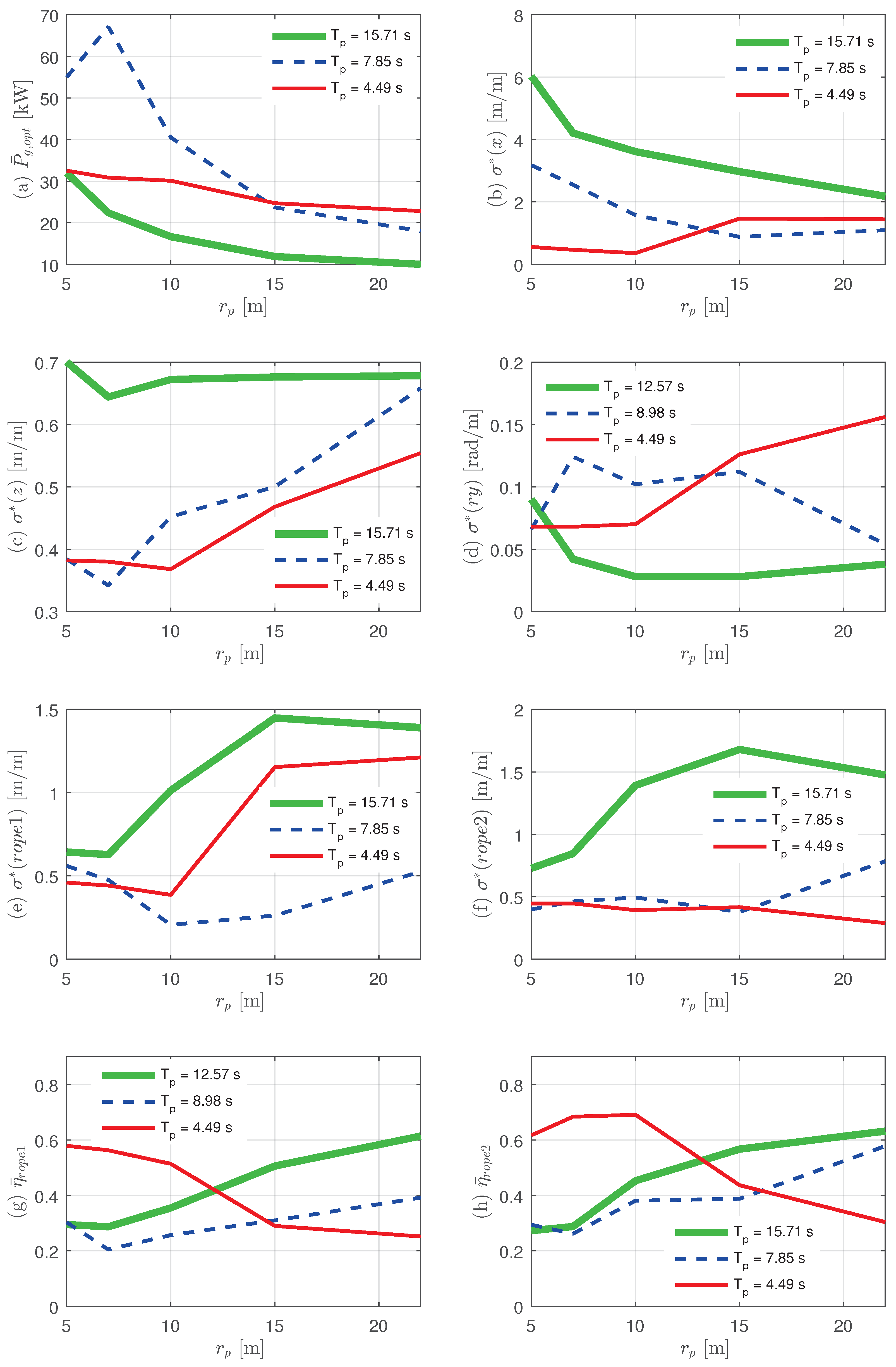
Figure 9.
Graphs of: (a) and (b) with varying counterweight mass for regular waves with .

Figure 10.
Graphs of mean and standard deviation of with varying wave direction at: (a) 15.71 s; (b) 7.85 s; (c) 4.49 s (thick green: average, red: standard deviation).
Figure 10.
Graphs of mean and standard deviation of with varying wave direction at: (a) 15.71 s; (b) 7.85 s; (c) 4.49 s (thick green: average, red: standard deviation).
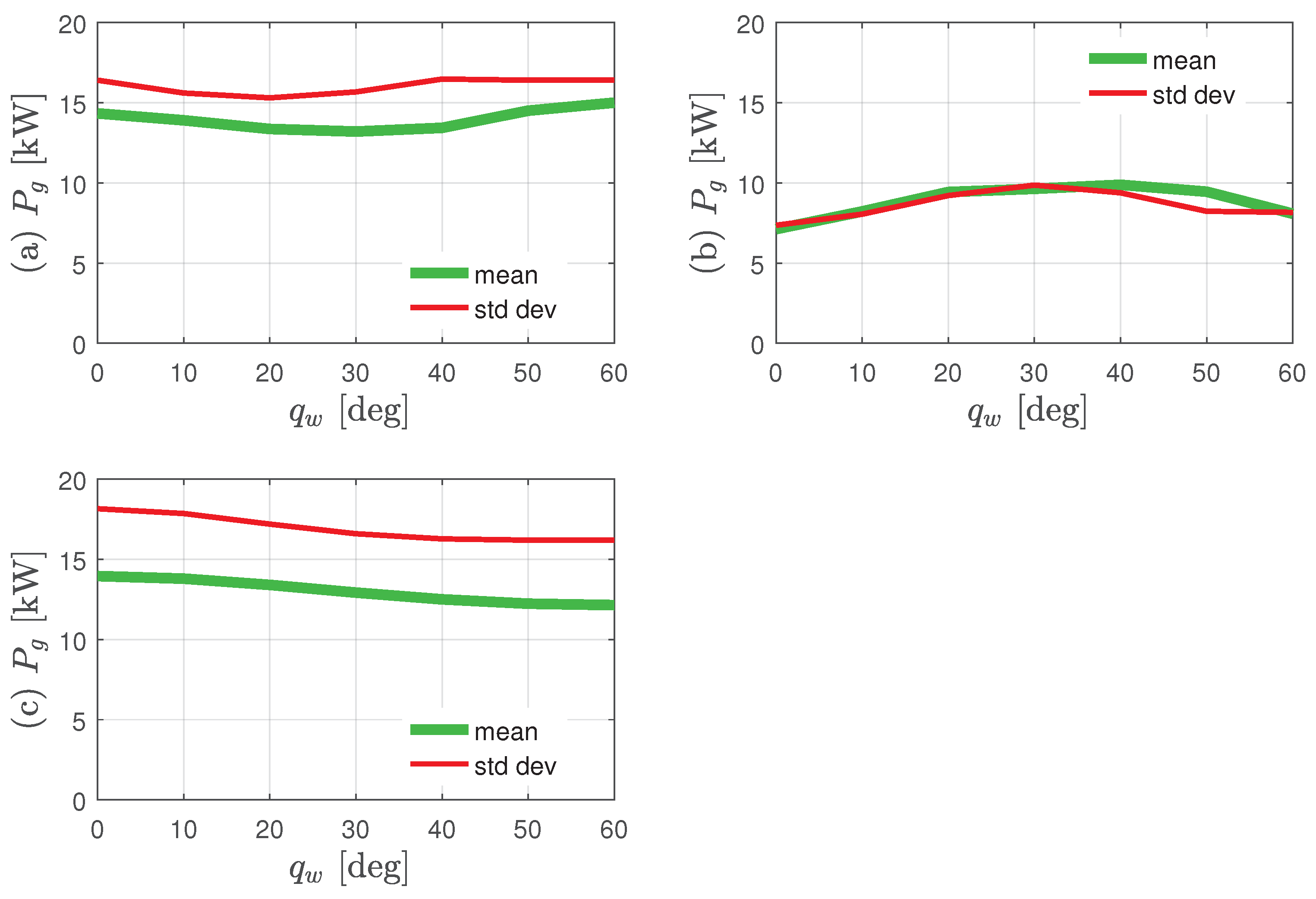
Figure 11.
Graphs of: (a) ; (b) CWR; and (c) with varying under JONSWAP irregular waves condition with .
Figure 11.
Graphs of: (a) ; (b) CWR; and (c) with varying under JONSWAP irregular waves condition with .
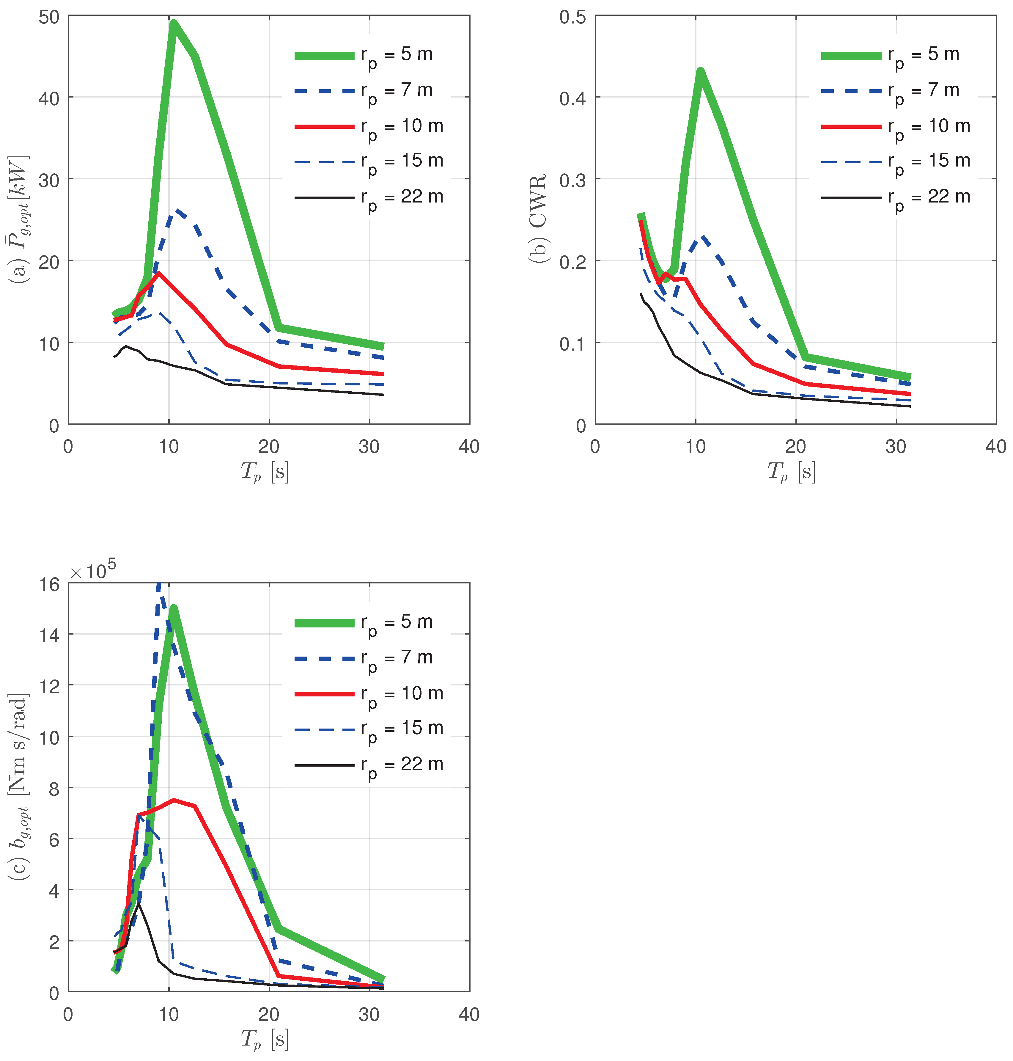
Figure 12.
Results of change at 15.71, 7.85, and 4.49 s under JONSWAP irregular waves condition with : (a) maximum average power; (b) in surge displacement; (c) in heave displacement; (d) in pitch displacement; (e) in rope 1 displacement; (f) in rope 2 displacement; (g) motion transfer efficiency of rope 1; and (h) motion transfer efficiency of rope 2.


Table 1.
Parameters and values in the simulations.
| Parameter | Symbol | Value | Unit |
|---|---|---|---|
| sea water density | 1025 | ||
| gravitational acceleration | g | 9.8 | |
| buoy radius | R | 6 | |
| buoy draft | d | 1 | |
| rope connection point from center | 5 | ||
| counterweight | 1000 (or 500, 2000, 4000) | ||
| buoy mass | (= | ||
| buoy inertia (rx, ry) | (=0.25 | kg·m | |
| buoy inertia (rz) | (=0.5 | kg·m | |
| distance of subsea pulley from center | 5, 7, 10, 15, 22 | ||
| sea depth | h | 10 | |
| rope pulley (drum) radious | 0.5 | ||
| gear ratio between pulley and generator | 1 | ||
| generator inertia | kg·m | ||
| virtual torsion spring coefficient | N·m/rad | ||
| generator damping load | – | Nm·s/rad | |
| wave direction | 0 (or 10, 20, 30, 40, 50, 60) | ||
| significant wave height | 1 | ||
| peak wave frequency | 0.2 to 1.4 | ||
| peak wave period | (=2 | 4.49 to 31.4 |
Table 2.
The pulley position and mooring angle.
| 5 | 7 | 10 | 15 | 22 | |
| 90 | 78.7 | 63.5 | 45 | 30.4 |
© 2017 by the authors. Licensee MDPI, Basel, Switzerland. This article is an open access article distributed under the terms and conditions of the Creative Commons Attribution (CC BY) license (http://creativecommons.org/licenses/by/4.0/).
Share and Cite
MDPI and ACS Style
Song, S.K.; Sung, Y.J.; Park, J.B. Numerical Modeling and 3D Investigation of INWAVE Device. Sustainability 2017, 9, 523. https://doi.org/10.3390/su9040523
AMA Style
Song SK, Sung YJ, Park JB. Numerical Modeling and 3D Investigation of INWAVE Device. Sustainability. 2017; 9(4):523. https://doi.org/10.3390/su9040523
Chicago/Turabian StyleSong, Seung Kwan, Yong Jun Sung, and Jin Bae Park. 2017. "Numerical Modeling and 3D Investigation of INWAVE Device" Sustainability 9, no. 4: 523. https://doi.org/10.3390/su9040523
Note that from the first issue of 2016, this journal uses article numbers instead of page numbers. See further details here.