
Optimization and Analysis of a Manufacturing–Remanufacturing–Transport–Warehousing System within a Closed-Loop Supply Chain

1
Industrial Engineering and Production Laboratory of Metz, Lorraine University, Ile du Saulcy, 57045 Metz CEDEX, France
2
Logistics and Transport Department, International University of Logistics and Transport, 51-168 Wroclaw, Poland
*
Author to whom correspondence should be addressed.
Sustainability 2017, 9(4), 561; https://doi.org/10.3390/su9040561
Submission received: 20 December 2016
/
Revised: 26 March 2017
/
Accepted: 30 March 2017
/
Published: 7 April 2017
(This article belongs to the Special Issue Sustainability in Supply Chain Management)
Abstract
:This paper deals with the optimization of a manufacturing–remanufacturing–transport–warehousing closed-loop supply chain, which is composed of two machines for manufacturing and remanufacturing, manufacturing stock, purchasing warehouse, transport vehicle and recovery inventory. The proposed system takes into account the return of used end-of-life products from the market. Manufactured and re-manufactured products are stored in the manufacturing stock. The used end-of-life products are stored in the recovery inventory for remanufacturing. The vehicle transports products from the manufacturing stock to the purchasing warehouse. The objective of this work is to simultaneously evaluate the optimal capacities of manufacturing stock, purchasing warehouse and the vehicle, as well as the optimal value of returned used end-of-life products. Those four decision variables minimize the total cost function. A discrete flow model, which is supposed to be the most realistic, is used to describe the system. An optimization program, based on a genetic algorithm, is developed to find the decision variables. Numerical results are presented to study the influence of transportation time, unit remanufacturing cost and configuration of the manufacturing/remanufacturing machines on the decision variables.
1. Introduction
Due to the increasing environmental preoccupation, the potential economic benefits and the legislation pressure, supply chain management has changed to focus on environmental impacts of production and earth resources’ preservation. Consequently, today, many managers are driving their supply chains through a sustainable supply chain management [1,2]. Several works have dealt with industrial sustainability. Despeisse et al. [3] have analyzed industrial practice and environmental principles, with the objective of developing a conceptual manufacturing ecosystem model as a foundation to improve environmental performance. The authors suggested a model that focuses on energy, waste and material flows to offer a better understanding of interactions between manufacturing operations, supporting facilities and surrounding buildings. Liu et al. [4] studied an operational decision-making problem of single machine systems with the consideration of sustainable performance. Bi-objective optimization model is elaborated to minimize the total completion time and total carbon dioxide emission. The authors have presented results that serve as a guide to implement sustainable production in factory companies and enrich the related theories of manufacturing decision. As far as this topic is concerned, throughout the last two decades, an interesting sustainable concept, which is called closed-loop supply chain [5], attracts more and more researchers and company leaders. Indeed, this sort of supply chain strengthened its position because of several evident advantages. Foremost, companies are obliged to pay attention to eco-destructive products, because environmental issues have become a major worldwide concern, for governments (laws and norms) as well as for consumers, who more and more take this point into account when they buy products. Moreover, they could benefit from the returns of broken or used products back to the retailer or even to the manufacturer. Last but not least, companies have realized an opportunity of raising profits and exploring new markets [6]. The reverse supply chain is the combination of both forward and reverse flows of products. The forward flow stands for products (or materials) going from suppliers through manufacturers and distributors to the consumers, and this flow corresponds to the market for “new” products. The backward flow (or reverse flow) is the back return of products from consumers, through collectors and recyclers, to suppliers or manufacturers. Returned products could be put back into distribution system later. In this case, we are talking about the market of used and/or recycled products. A reverse supply chain implies a relationship between these two markets and, when they coincide, we talk of a closed-loop network, instead of an open-loop network [7]. Indeed, in such supply chains, four major categories of return items have been defined: recycling of wasted products, reusable products, repair services and remanufacturing. Concerning the recycling, the returned product completely disappears, and only raw material reappears in the production circuit. Reusable products can reappear in the same state as when they had been returned, as it is the case for pallets or returnable bottles. Concerning the repair services, the returned product is destined to be sent back to the owner after repairing. It often concerns products under guarantee. In this paper, we will consider the case of remanufacturing closed-loop supply chain. Remanufacturing is an industrial process in which used end-of-life products are restored to “like-new” conditions [8]. This process has existed for years, especially for high-value items, such as locomotive engines and aircrafts (product life extension) [9], and it is spreading into more industries and product sectors than ever before.
Within the past decade, remanufacturing closed-loop supply chains have drawn the attention of academia and manufacturers due to their great performance in raising profits and improving ecology. In the literature, we have found many works that consider such systems. Mitra [10] studied the inventory management issue in closed-loop supply chains, and developed deterministic and stochastic models for a two-echelon system, with correlated demands and returns, under generalized cost structures. More recently, Kenné, Dejax, and Gharbi [11] have proposed a production-planning model of a hybrid manufacturing/remanufacturing system in a continuous time stochastic context. The authors used hedging a point policy to determine the optimal stock levels of manufactured and remanufactured products. These optimal stock levels control production rates. Chung et al. [12] analyzed an inventory system with traditional forward-oriented material flow, as well as a reverse material flow supply chain. In the reverse material flow, used products are returned, remanufactured and shipped to the retailer for resale. Turki et al. [13] considered a closed-loop supply chain system with remanufacturing activities. The authors have evaluated the optimal serviceable inventory level, which allows for minimizing the sum of inventory, lost sales costs, and machines degradation cost. More recently, Turki and Rezg [14] studied a manufacturing/remanufacturing system, taking into account the withdrawn products and the return of the used products from the market. The authors studied the influence of withdrawn products and used products on the value of the optimal serviceable inventory level. However, the majority of these works consider classical remanufacturing supply chain system composed of two machines (manufacturing and remanufacturing) and one serviceable stock. In such systems, several characteristics of supply chain are not considered, such as the purchasing warehouse inventory or the transportation activities. However, delivery or transport time [15], which is the amount of time the vehicle needs to move the products between a manufacturing stock and a purchasing warehouse, has a great impact on the systems’ performance.
There are works studying the impact of transportation time or lead-time on the whole system. For instance, Teunter [16] studies a simple manufacturing/remanufacturing system with disposal option, deterministic demand and lead times to investigate inventory replenishment policies. Tang and Grubbström [17] explored a coordination problem in a two-level assembly system that has stochastic transport times and developed models to minimize total stock out and inventory holding cost. Later, Tang and Grubbström [18] adopted this method to study a manufacturing/remanufacturing system with stochastic transportation times and constant demand. The authors compared the two different ordering policies (cycle ordering policy and dual sourcing), and showed the influence of transport time values on economic consequences. There are also other works in that area. However, apart from the transport time or delivery time there are also other main characteristics of transportation activity, such as vehicle capacity and transportation costs, which are not often taken into account. In this paper, we consider a remanufacturing closed-loop supply chain that ensures production, transport and selling of products under optimal economic management. The configuration of this supply chain system is inspired by the real case of a company that produces new products from raw material and used products, then transports the products from the manufacturing stock to the purchase warehouse which is usually located in an urban area. Examples include companies that produce mobile phones, printer cartridges, home appliances or car spare parts. Indeed, when warehouses are located in city centers, where traffic is more constrained, vehicle capacities and transportation time become two considerable issues to take into account. Thus, in this work, we will consider a deterministic transportation time, we will include transportation costs and, among other things, we take interest to optimize the vehicle’s capacity. Moreover, we also optimize the capacities of manufacturing and purchasing warehouses included in our system, because their levels are also usually limited and because they have a significant impact on economic indicators. To study the benefit of remanufacturing used end-of-life products versus to the manufacturing products from raw materials, we include unit costs of manufacturing and remanufacturing as well as costs for collecting the used end-of-life products in the total cost function. Concerning the return of the used end-of-life products, several works assume that the returned quantity is proportional to customers demand and is defined by a percentage relative to the demand [11,14,19], while others [20,21] consider the returned quantity for remanufacturing restricted by the sales in previous periods. Indeed, sales quantity is lower than the demand when a part or the whole of the latter is unsatisfied (lost sales). Therefore, returned quantity of used end-of-life products is based on the sales in past periods, and not based on demands. In this paper, to consider the system which is more realistic, we assume that the returned quantity is propositional to the sales in the previous periods. The modeling of such complex closed-loop supply chains requires the use of a discrete flow model.
Discrete flow model is widely used for the design, the optimal control and the optimization of manufacturing systems. It has been considered as an alternative paradigm to queuing network for analysis and synthesis of discrete event systems. This model is also used for network systems designs or for modeling manufacturing/remanufacturing systems [22]. Indeed, a discrete flow model is more realistic for discrete manufacturing systems than for continuous flow models (Yao and Cassandras [23], and Xie, Hennequin, and Mourani [24]); allows tracking individual parts, in either performance evaluation or real-time flow control; and is generally easier to simulate. However, in terms of optimization, continuous parameter optimization is usually easier than discrete parameter optimization [25]. That is why we spent much time on choosing the optimization technique and our final choice was a genetic algorithm method.
Genetic algorithms are useful and relevant for discrete optimization purpose. Many applications of this method proved both its accuracy and speed [26,27]. The particular shape of the objective function in the neighborhood of optimal solutions and the relatively long computation time of the objective function calculating program made us propose adding to this genetic algorithm a neighborhood method, in a second phase of optimization.
This article brings three contributions: the first is to consider a manufacturing/remanufacturing closed-loop supply chain in a sustainable framework, whilst taking into account the transport and the warehousing of new products, and the recovering of used end-of-life products. It consists simultaneously to determine the values of four decision variables: the optimal levels of the manufacturing stock and purchasing warehouse, the optimal transport vehicle capacity and the optimal percentage of returned used end-of-life products. The consideration and determination of these decision variables and study of such manufacturing/remanufacturing closed-loop supply chain is a novelty in industrial sustainability topics and a challenging problem to solve. Indeed, the coordination between manufacturing/remanufacturing operations, the storage and the transport in presence of return of used end-of-life products complicates the inventory control and production decisions. The second contribution is to establish discrete flow model that describe closed-loop supply chain and its coordination, and then to determine decision variables using an optimization method based on a genetic algorithm. The third contribution is to study the impact of the transportation time, unit remanufacturing cost and the reconfiguration of the machines on the optimal capacities of the manufacturing stock, the purchasing warehouse, transport vehicle and optimal return percentage of used end-of-life products.
The article is organized as follows: we introduce the manufacturing–remanufacturing–transport–warehousing closed-loop supply chain in Section 2. We then explain the optimization performed on this model with a genetic algorithm in Section 3, before introducing and analyzing the numerical results in Section 4. We finally conclude in Section 5 and consider some further research axes and perspectives.
2. Manufacturing–Remanufacturing–Transport–Warehousing Closed-Loop Supply Chain System
2.1. Notation
| t | instant time. |
| ∆t | time period length. |
| s(t) | manufacturing stock (B) level at time t. |
| S | manufacturing stock capacity. |
| S* | optimal manufacturing stock capacity. |
| g(t) | amount of products outgoing from manufacturing stock S at time t. |
| r(t) | returned products inventory (R) level at time t. |
| D | customers demand at every time t. |
| y(t) | satisfied demand at time t. |
| l(t) | unsatisfied demand at time t. |
| w(t) | purchasing warehouse (W) level at time t. |
| z(t) | returned amount of used end-of-life products at time t. |
| p | percentage relative to the sales of the returned used end-of-life products. |
| p* | optimal percentage relative to the sales of the returned used end-of-life products. |
| q(t) | products being transported at time t. |
| τ | transportation time (the value of transportation time is multiple of Δt). |
| θ | products’ service life. |
| X | purchasing warehouse capacity. |
| X* | optimal purchasing warehouse capacity. |
| V | vehicle capacity. |
| V* | optimal vehicle capacity. |
| α(t) | state of the machine M1 at time t. |
| β(t) | state of the machine M2 at time t. |
| U | maximum production rate of both machines. |
| U1 | maximum production rate of the machine M1. |
| U2 | maximum production rate of the machine M2. |
| u(t) | production rate of M1 and M2 at time t. |
| u1(t) | production rate of the machine M1 at time t. |
| u2(t) | production rate of the machine M2 at time t. |
| MTBF1 | mean time between failures for machine M1. |
| MTBF2 | mean time between failures for machine M2. |
| MTTR1 | mean time to repair for machine M1. |
| MTTR2 | mean time to repair for machine M2. |
| cs | unit inventory holding cost for the manufacturing stock (B). |
| cl | unit lost sales cost. |
| cr | unit inventory holding cost for the returned products (recovery inventory R). |
| ct | unit transportation cost. |
| cw | unit inventory holding cost for purchasing warehouse (W). |
| cu1 | unit manufacturing cost of a product from raw materials. |
| cu2 | unit remanufacturing cost. |
| cz | unit return cost of used products. |
| T | total simulation time. |
| f(t) | cost function at time t. |
| F(T) | total cost function (the objective function). |
Decision variables are S*, X*, V* and p*.
2.2. Explanation of the System
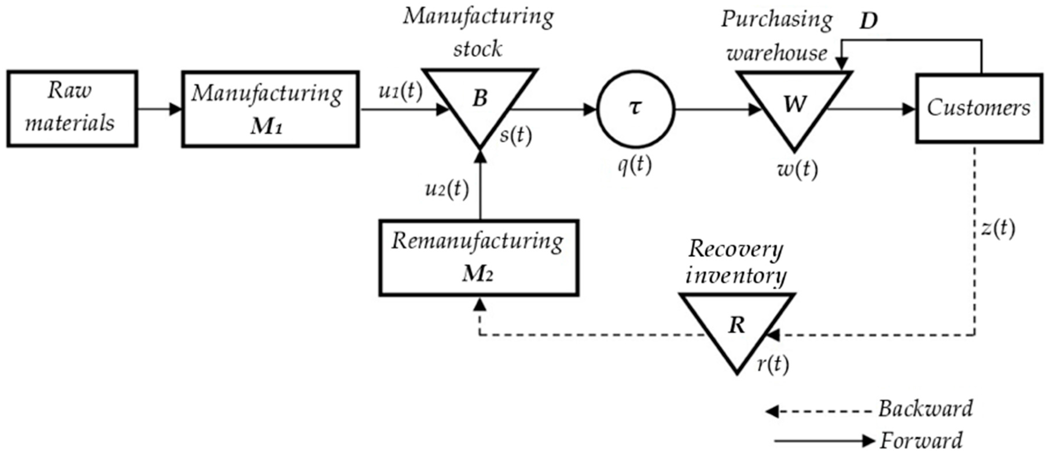
The studied closed-loop supply chain system (see Figure 1) consists of two parallel machines (denoted M1 and M2, for manufacturing and remanufacturing, respectively), which are subject to random repairs and failures. Both machines are assumed to produce the same type of product. Machine M1 produces from raw materials and machine M2 produces from used products that were returned (end-of-life products). Indeed, in this closed-loop supply chain system, the production activity is considered in forward and reverse directions. Remanufactured products are of the same quality as the products that are made from raw materials. Therefore, both types of products (manufactured and remanufactured) can be distributed like new. At every time t, customers demand a constant quantity of products D, which is satisfied from the purchasing warehouse W. Machines M1 and M2 are filling up the manufacturing stock B that supplies the purchasing warehouse W with a transport vehicle. Thus, products outgoing from B are transported to the warehouse, and take a transportation time τ to arrive to W. Indeed, when the products leave S at time t, they will arrive at time t + τ. The vehicle has a maximum capacity V and transports a quantity of products q(t) at time t between B and W. The maximum capacity of purchasing warehouse W is defined by variable X. Another inventory R is available for stock keeping of the returned used end-of-life products, before their remanufacturing process. It is assumed that inventory R has an infinite capacity. As mentioned in the introduction, to study more realistic situations, we calculate z(t) at every time period, with taking into account the lost sales that have occurred.
Let [0, T] be the finite horizon discretized into K periods Δt (see Figure 2). Indeed, Δt is the time period length that represents simulation time step, thus the total simulation time T = K·Δt. Occurrence of the events in system (machine failure, stock empty, etc.) is defined by the instant time t є [0, T].
Possible system events at every time t are: machine M1 failure, machine M1 repair, machine M2 failure, machine M2 repair, manufacturing stock full, manufacturing stock full empty, purchasing warehouse full, purchasing warehouse empty, lost sales, products transport, return of used products, recovery inventory full, recovery inventory empty, manufacturing of products and remanufacturing of used products.
We suppose that machine M1 will never starve. M1 is either up or down.
Machine M1 state at time t is represented by:
The machine M2 state at time t is represented by:
Time to repair and time between failures are exponentially distributed. In the case that machine M1 is up, production rate u1(t) can be between 0 and its maximum U1, i.e., 0 u1(t) U1. In the case that machine M1 is down, u1(t) = 0. Machine M2 is in the same case, where u2(t) is its production rate and U2 is its maximum production rate. The failure/repair process is an independent random process.
We consider the following assumptions:
- (1)
- In order to simplify the calculations, we assume Δt = 1.
- (2)
- When the demand is not satisfied, loss occurs which results into lost sales costs (l(t)).
- (3)
- To consider transportation time, we assume that τ > 0, known and constant. Indeed, τ is multiple of Δt with τ = m·Δt = m (Δt = 1) and m = {1, 2, 3, …, T}. We assume also that the time for changing and discharging the vehicle is included in the transportation time τ.
- (4)
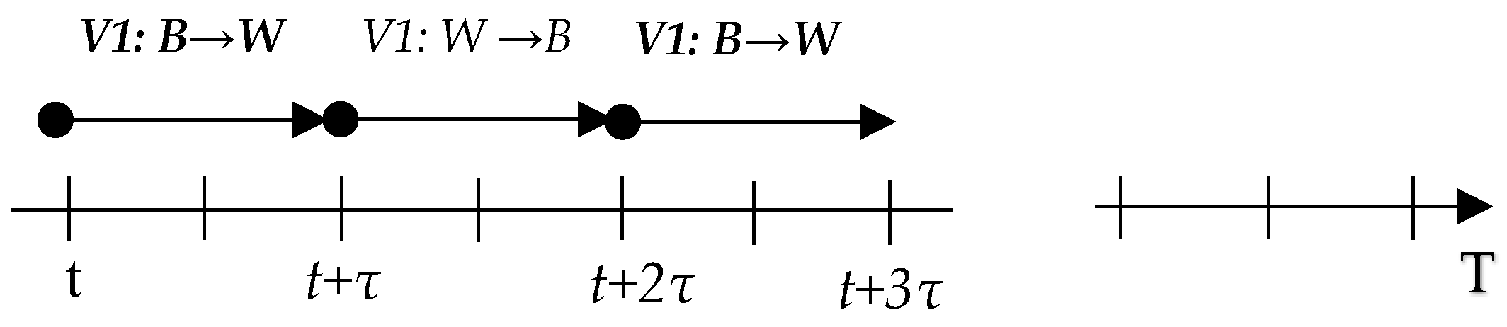
- We assume the case where transport is ensured by two vehicles, vehicle 1 and vehicle 2. When vehicle 1 reaches W, vehicle 2 departs from B and when vehicle 1 comes back to B, vehicle 2 reaches W and vice versa. This assumption allows having one trip from B to W for every τ period and the objective is to reduce the number of trips (see Figure 3: an example when m = 2 we have τ = 2·Δt = 2). This assumption is the usual case of companies that ensure manufacturing and transport of products.
- (5)
- Companies are working to keep a good level service by satisfying customers’ demands. Thus, in inventory management, to avoid having too much lost sales (unsatisfied demand), we must avoid having both manufacturing stock B and purchasing warehouse W is always empty. Thus, we made the following assumptions:
- (5.1)
- Maximum production rate U satisfies the demand (i.e., U ≥ D). This assumption avoids having manufacturing stock B always empty.
- (5.2)
- Purchasing of the warehouse capacity W should be equal or higher than the sum of demands during the transportation time (i.e., X ≥ τ·D). Indeed, the fact that W satisfies the customers demand D at each period and is fulfilled every period equals to the transport time τ = m·Δt. The level of W should be equal or higher than the sum of demands during τ (w(t) ≥ m·D) to satisfy the demands. Thus, if capacity X < τ·D, we always have lost sales. Let us look at the following example (see Figure 4).
If we assume that m = 2 (i.e., τ = 2·Δt = 2) and D = 10 products/period, at the purchasing warehouse, the capacity should be X ≥ τ·D = 2 × 10 = 20.- (5.3)
- The vehicle capacity should also be equal or higher than the sum of the demands during the transportation time (i.e., V ≥ τ·D). Indeed, the vehicle supplies the purchasing warehouse W. If V < τ·D, the level of W will never reach τ·D, and then we always have lost sales.
- (6)
- Maximum production rate U2 is higher than the return amount, (i.e., U2 > z). This assumption avoids having the remanufacturing inventory R always full.
- (7)
- Remanufactured products have the same quality and price as the brand new ones.
- (8)
- We suppose that we have enough parts in the warehouse to satisfy the demand in a given time period t = 0, i.e., w(0) ≥ D.
2.3. Mathematical Model
As mentioned in our introduction, we use a discrete flow model to formulate the problem. Assumptions in this model are the same as those presented in the beginning of Section 2.
As mentioned above, the studied time horizon is discretized in equal periods. We should also emphasize the fact that, in our model, demand D is always satisfied at the beginning of each period, which means that we use the purchasing warehouse level of the previous period w(t − ∆t). Thus, the value of satisfied demand at time t could be found with following equation:
The Purchasing warehouse W, which satisfies customers’ demand, is replenished with products coming from the manufacturing stock and being transported by the vehicle. Thus, the purchasing warehouse level at time t (w(t)) is the sum of the amount of products in this warehouse remaining from the previous period (t − ∆t), and of the amount of products that left manufacturing stock at time (t − τ), minus the amount of products that were sold in the current period:
The transportation time τ can obviously take values greater than 1. Thus, we need to note that, if (t − τ) < 0, then g(t − τ) = 0.
However, if (t − τ) = 0, we are obliged to set boundaries for g(0), assuming that the transportation from the manufacturing stock (B) to the purchasing warehouse (W) has the frequency of τ, thus and , so .
The purchasing warehouse level, after the transportation and the satisfaction of the demands during period τ, is given by:
Remark 1.
We introduced this equation because it is needed for further calculations.
Outgoing products from manufacturing stock B at time t need time τ to be transported to the purchasing warehouse W. The amount of products outgoing from manufacturing stock S at time t (g(t)) depends on the purchasing warehouse level at time t + τ and its total capacity, manufacturing stock level at time t − ∆t , vehicle capacity and the demand:
With n = {1, 2, 3, …, [T/τ]}, where [T/τ] is the integer part of T/τ and is the number of transportations during the finite time horizon [0,T]. Thus, g(t) = 0 when and means that the products outgoing from B at each period τ (see Assumption 3).
The Products from machines M1 and M2 replenish the manufacturing stock S which supplies the purchasing warehouse.
Therefore, the manufacturing stock level at time t consists of the level of this stock remained from the previous period, plus the quantity of products that was produced during the previous period, minus the amount of products outgoing from manufacturing stock S at time t:
The amount of unsatisfied demand (lost sales) at time t and is calculated by subtracting the amount of products that were sold at time t from the customers’ demand:
The number of returned used end-of-life products at time t (see Figure 5) is proportional to the quantity of sold products at time t − θ (when the products were sold to the customer). We denote by p (0 < p < 1) the percentage of products which are returned for remanufacturing relatively to sales. As it was mentioned above, θ stands for the products’ service time. Obviously, in case if (t − θ) < 0, there are no returns.
In the following figure, we illustrate the products’ sales and returns (e.g., θ = 3).
The returned products inventory R, which supplies the machine M2, is replenished by the returned products z(t). Thus, the returned products inventory level at time t consists of the level of this inventory that remained from the previous period, plus the amount of the products that were returned in the current period, minus the amount of products that were used by the remanufacturing machine M2 on the previous period:
We consider that the parts are transported in a vehicle. The amount of products that entered the vehicle at time t is the amount of parts being transported during the time . That is to say, the shipment enters the vehicle at time (n·τ) and the next shipment enters another vehicle at time (n + 1)·τ.
The number of products being transported at time t is described as follows:
As described above, n = {1, 2, 3, …, [T/τ]}, where [T/τ] is the integer part of T/τ and is the number of transportations during the finite time horizon [0, T].
For machines productions rates, we use the hedging point policy [28], which ensures that the amount of products does not exceed the manufacturing stock capacity.
In order to determine the production rates for M1 and M2 while both machines are working we need to introduce a partitioning policy. Therefore, we assume that:
and
We are now going to explain the production control of both machines, according to machines states and inventories cases. This policy controls machines production, with preserving coordination between manufacturing, remanufacturing, inventorying and return of end-of-life products.
Transforming the previous equations, we can determine the production rates of M1 and M2 separately:
Cost function at time t, which consists of inventory costs (manufacturing stock, returned products inventory, purchasing warehouse), transportation cost, lost sales costs, manufacturing/remanufacturing costs and return of used products cost:
The total cost function (the objective function) and is given by:
where T is the total simulation time.
3. Optimization Based on the Genetic Algorithm
3.1. Interest of Using Optimization Method
Total function cost program has been encoded with the C++ freeware devcpp (Free Software Foundation, Inc., Cambridge, MA, USA). Since the model is a stochastic one, we decided to take as objective function the average value of ten simulations. Even though this decision makes the calculation time longer, it has the advantage of a better accuracy and confidence in obtained results. Indeed, in order to obtain efficient simulation results, we have launched several simulations, with different combinations of both time horizon and repetitive sets, to find the suitable couple of values, which is the compromise between spent time and calculation accuracy. In our work, the time horizon has been found to be 105 time units, and we come to an average of ten simulations per set of input parameters. With simulation, we verified that obtained results are efficient. For simulation purpose, this function is called with different parameters sets. Furthermore, when an optimal vector value is researched, simulations are performed with all the possible parameters sets. Since the solution space is very wide, we use optimization techniques to reduce the number of simulations, and therefore lessen necessary time to get the optimal vector.
However, this stochastic objective function also presents a drawback obtaining two different values for the same input vector. This is not only harmful for the calculation, but also for optimization purpose, because the neighborhood of optimal solution is rather flat. Then, while a better input vector is tested, it may not be retained only because the objective function returned value is overvalued.
Nevertheless, the gain obtained on computation time using our optimization method overtakes the stochastic objective function and the flat optimal solution neighborhood drawbacks. This is the reason why we use an optimization method to converge quickly towards an optimal solution. Moreover, we developed improvement methods which, in this area, find better solutions while testing the less possible vectors.
3.2. Optimization Method Description
We decided to tackle the optimization problem with four discrete variables. Each of the three variables S*, X* and V* can take integer values in the interval [10; 100], and the fourth variable p can take one of the five first integer values. Two optimization constraints are added to the problem. The first (V* ≤ S*) stands for the fact that the vehicle capacity must be inferior or equal to the manufacturing stock. The second constraint (V* ≤ X*) reminds that the vehicle capacity must also be inferior to the purchasing warehouse capacity. To respect both constraints and chromosomes simplicity, we decided to generate canonical individuates, and to test their conformity to problem constraints only after their generation. Obviously, not fitting individuates did not give rise to the objective function evaluation. Resulting solutions space distortion of this programming strategy has only a weak incidence on final results, because neighborhood strategies are very effective and the genetic algorithm is only used to speed up the solution process.
The optimization algorithm we developed is described below (Algorithm 1):
| Algorithm 1 Optimization Algorithm Pseudo-Code |
|
In the first step of the metaheuristic, we optimize using a classical genetic algorithm (Lines 1–2) with a population of 30 individuates and a stopping criteria counting the number of times when the best obtained value remains identical ctbvi (counter of times when best value remains identical) = 6 [29,30,31,32]. However, since the objective function evaluation is rather long, we quickly shift on the second step, composed of neighborhood tests. The second step is the most effective neighborhood we have tested (Improvement method 1, on lines 3–17). Here, we suggest moving two randomly chosen coordinates of the vector, either upper or lower from current vector position. Variations authorized are successively decreasing from 100% of the difference between coordinate position and its corresponding bound to, respectively, 50%, 33%, 25% and 20%. Tested coordinate value is then randomly drawn in the authorized variation interval. At each time, a best individuate is found, it becomes the new reference point in solution space, from which neighborhoods are tested. The third step of the optimization method moves coordinates only one by one, in both possible directions (Improvement method 2, on lines 18–38). It is repeated as long as it improves the current solution. Variations authorized for this improvement method are less and less wide, because it is performed at the end of the optimization process. At each step of the optimization process, only fitting individuates are tested, because of the relatively long objective function computing time.
3.3. Conclusion on Optimization Method
Obviously, genetic algorithm methods are stochastic, as well as neighborhood methods. Thus, the final results cannot be considered as optimal. Nevertheless, in this particular context of long computing time of objective function, the optimization method we have developed allows converging towards the area of optimal solution by testing less than 1% of the solution space. We can also add that the objective function is all but convex. Moreover, it is quite flat around optimal solution. In addition, numerous quasi-optimal solutions are relatively remote. Despite all these drawbacks, the method we propose correctly optimizes, which tends to prove its relevance to treat this kind of problems.
4. Numerical Results
In this section, we will introduce some numerical data and apply the above-described model to compute the decision variables. We also conducted several important studies. Firstly, we examined an influence of p value (returned end-of-life products percentage) on optimal values of manufacturing stock (S*), vehicles’ capacity (V*) and purchasing warehouse (X*). We do not assume here that we can have an impact on the value of p, because it is a given value (by environmental regulations, the company’s policy, etc.). We just study its impact on the system’s outcomes. Secondly, an influence of the value of τ (transportation time) on the optimal values of returned products percentage (p*), manufacturing stock (S*), vehicles’ capacity (V*) and purchasing warehouse (X*) has been analyzed. Here, we assume that the returned products percentage p is under our control and we can optimize this parameter, among others, to achieve the most effective system state possible. Finally, we observed the influence of unit manufacturing and unit remanufacturing costs on optimal values p*, S*, V*, and X*. We gradually increased these costs and then noticed that they have a significant impact on the system’s indicators.
4.1. Influence of p on the Optimal Values S*, V*, X*.
To conduct this study, five different percentages were applied on p that are 10%, 20%, 30%, 40%, and 50%.
The input data that we used for the simulation and optimization are the following:
- T = 100,000 periods
- MTBF1 = 4 periods
- MTTR1 = 1 period
- MTBF2 = 4 periods
- MTTR2 = 1 period
- D = 10 products/period
- U1 = 9 products/period
- U2 = 5 products/period
- τ = 1 period
- cu1 = 10 monetary units
- cu2 = 4 monetary units
- cw = 2 monetary units
- cs = 2 monetary units
- cr = 1 monetary unit
- cz = 1 monetary unit
- cl = 250 monetary units
- cq = 1 monetary unit
- θ = 30 periods
After the simulation and the optimization processes, we have obtained the following results.
As can be noticed in Table 1, the increase of the percentage of returned products tends to decrease optimal values. This can be explained by the fact that when p increases, the amount of returned used end-of-life (z(t)) increases and then recovery inventory fills up more. Thus, M2 is better supplied and production quantities M2 may increase. This is why manufacturing stock (B) fulfillment becomes more stable and, consequently, the customers’ demand is better satisfied (less lost sales). However, even though lost sales costs decrease, inventory holding costs in B, X and R may grow up. Therefore, to counterbalance this increase, optimal inventory capacities S* and X* decrease. This is confirmed in the work [12]. The value of optimal vehicle capacity V* follows behaviors of S* and X*, because the vehicle ensures the supply of W from B. Thus, V* decreases, when S* or X* decreases, and vice versa.
The most interesting aspect in this example is that the total cost F(T) has a minimum when p = 20% (see Table 1). That corresponds to the optimal return of used end-of-life products for our closed-loop supply chain. Indeed, when p = 10%, the return of used products is low and machine M2 is insufficiently supplied, thus production rate decreases and then B and W are insufficiently supplied. Results are number of unsatisfied demands and then lost sales cost become important. Therefore, in this case, total cost is higher than when p = 20%. In the case where p > 20%, machine M2 is sufficiently supplied and then B and W are sufficiently supplied. Thus, demands are satisfied as when p = 20%, but of used end-of-life products return become more important, thus increasing used products return cost and the recovery inventory cost. Thus, in this case the total cost is higher than when p = 20%. Therefore, by way of conclusion we can say that the total cost can be optimized in function of the returned products amount. Thus, in the case where the enterprise leader has the option to fix the amount of returned used products, he can optimize the system by determining the optimal value of p that minimizes the total cost. This is what studied in the next parts.
4.2. Influence of the Value of Transportation Time (τ) on the Optimal Values p*, S*, V*, and X*
For this study, we varied τ (transportation time) and included p* as decision variable into the optimization algorithm. Input data are the same as in the previous part. Results are presented in Table 2.
This part has some interesting information and we should pay attention to it. First, we need to mentio, that we have introduced another column—X*/(τ·D). This column shows the ratio of the optimal capacity of the purchasing warehouse to the demand throughout the time period of τ (recall that in our model vehicle departures occur every τ period, so we need to have τ·D products in the purchasing warehouse in order to satisfy all the demand). The higher the value of this ratio, the more extra capacity we have in the purchasing warehouse.
As can be seen in the Table 2, when transportation time increases, S*, V* and X* increase too. This is normal because during the transportation time, inventories shall hold a quantity equal or higher to τ·D (see assumptions), then optimal capacities increase with τ. We can notice that τ has hardly any influence on P*. This is due to the fact that at every time t, we have an amount of used products return to R that supplies machine M2 independently on transportation time τ. Total cost normally increases with transportation time, because in this case transport cost and inventory cost increase with τ.
In the first case with τ = 1, we can notice that optimal purchasing warehouse capacity is much higher than optimal manufacturing stock capacity (X* > S*). Consequently, the ratio is also high. This phenomenon can be explained in the following way. It is a well-known fact in inventory management that, under uncertain demand, inventory level should be higher than this demand. In our model, in the case with τ = 1 (which means that transportation takes place every time period and immediately after production), great fluctuations in manufacturing stock (B) occur and consequently, the model creates a considerable level at the purchasing warehouse (W) to mitigate those fluctuations. This observation is evidenced by other results. We can see, in Table 2, that in cases with τ > 1, we have more chances to stabilize and control production, because we have more time. Thus, we also have greater possibility to fulfill the purchasing warehouse (W) to the desired level, thus avoiding to create a huge level. Moreover, the higher the value of τ is, the better we can control the production is possible and the values of S* and X* get closer to the amount of stock that we will achieve in perfect situation (i.e., M1 and M2 never fail). We can see this from the last column of Table 2, where the ratio is approaching the value of 1, which is the value of a perfect situation. To illustrate this, we provide some examples.
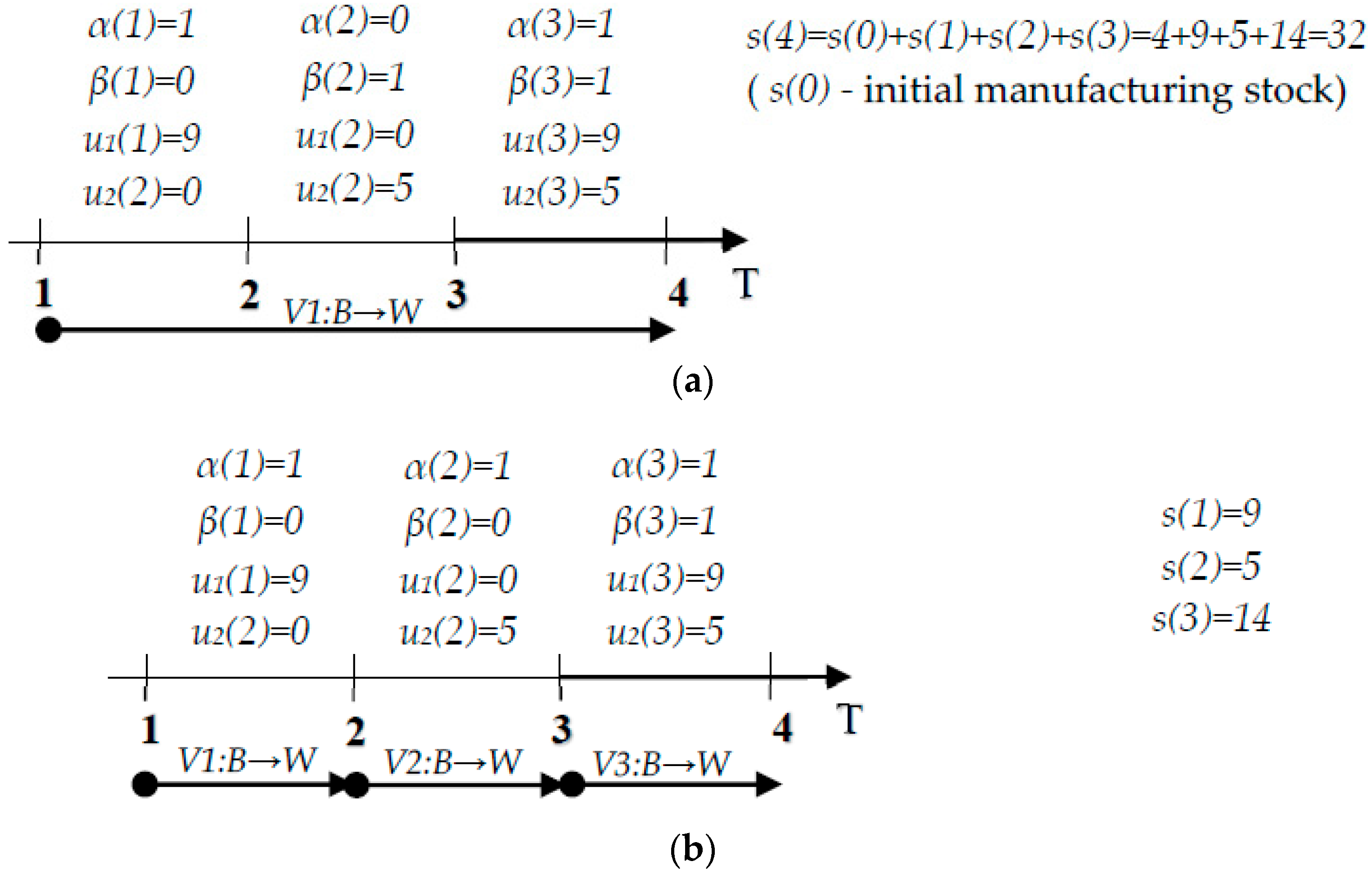
We assume two situations with: (a) τ = 3, D = 10 and s(0) = 4; and (b) τ = 1, D = 10 and s(0) = 4.
We assume that, in Case (a), the last departure of the vehicle occurred at t = 1. Thus, the next are takes place at t = 4 (because τ = 3). In addition, as far as τ = 3, the needed desirable amount of products to transport to the purchasing warehouse is τ·D = 30 products. Therefore, to satisfy this demand we need to produce sufficient amount during periods t = 1, t = 2 and t = 3. In Case (b), departure of vehicle occurs in the beginning of every period (τ = 1), then desirable amount of products to transport to the purchasing warehouse is τ·D = 10 products. In addition, we only have one time period to produce a sufficient amount of products. If the situation is perfect and machines never fail, the production rates in both cases would be divided between the machines in such a way that they would always satisfy the demand with a minimum or no stock level. However, as far as machine can fail, the stock level becomes essential. Nevertheless, the more time we have between the two consecutive vehicle departures, the more production control is possible. If we look at Figure 6a,b, we can see that when τ = 1, quantities of products entering the vehicle before its departure are very different, which leads to either shortages or high stock levels. Furthermore, on the contrary, when τ = 3 the quantity of products entering vehicle stabilizes. Stock level is not so big, which allows reducing the inventory holding costs. In conclusion, the more transportation time increases the more the production is controlled to satisfy the demand, and then the optimal inventories and transport capacities are easy to evaluate.
Finally, we are obliged to emphasize the fact that, in results from Table 2, the values of X* and S* are equal (excepted when τ = 1). This is because we have the same unit inventory holding cost in manufacturing stock and purchasing warehouse (i.e., cw = cs). Variation of those costs would change the situation. For example, we considered the same input data, changing only the values of cw and cs.
Therefore, from results presented in Table 3, we can see that when the unit holding cost in manufacturing stock (cs) is lower than in the purchasing warehouse (cw), the optimal capacities of those two stocks no longer remain equal, as seen in Table 2. This makes sense, because, even though cw gets bigger, the model still needs to create a considerable stock level and, thus, to counterbalance this cost increasing in purchasing warehouse, it transfers a part of this stock to manufacturing stock. In the second case, we observe the opposite situation with cs > cw and therefore X* gets higher than S*. These results prove that our model has an appropriate behavior in function of relative variations of parameters cs and cw.
4.3. Influence of Machines Reconfiguration and Unit Manufacturing/Remanufacturing Costs on the Optimal Values p*, S*, V* and X*
The remanufacturing of used end-of-life items improves the sustainability system by reducing the consumption of row materials and the recovery of the used products. In this part, we will study the influence of remanufacturing production () on the system by increasing remanufacturing compared with the manufacturing (). The idea is to change the configuration of the machines by increasing the maximal production rate of machine M2 (U2) and decreasing maximal the production rate of machine M1 (U1), while preserving their sum value (i.e., U = U1 + U2 stays constant). Then, for every reconfiguration, we determine the total cost and the system optimal outcomes (see Table 4). In the second part, we will study the influence of remanufacturing cost versus manufacturing cost on the system. Thus, we vary units manufacturing and remanufacturing costs to study their influence on the system optimal outcomes.
As can be observed in Table 4, when the remanufacturing of used products increases compared to the manufacturing, optimal return of used products increases and total cost of course decreases. Indeed, because the unit remanufacturing cost is much lower than the unit manufacturing cost (cu2 < cu1), the model tends to shift more production activity to M2. Thus, we were interested in studying the influence of units manufacturing and remanufacturing costs on machines configuration. We changed its value from cu2 = 4 to cu2 = 8.
We have studied four configurations of the machines:
- (1)
- U1 = 9 and U2 = 5;
- (2)
- U1 = 8 and U2 = 6;
- (3)
- U1 = 7 and U2 = 7; and
- (4)
- U1 = 6 and U2 = 8.
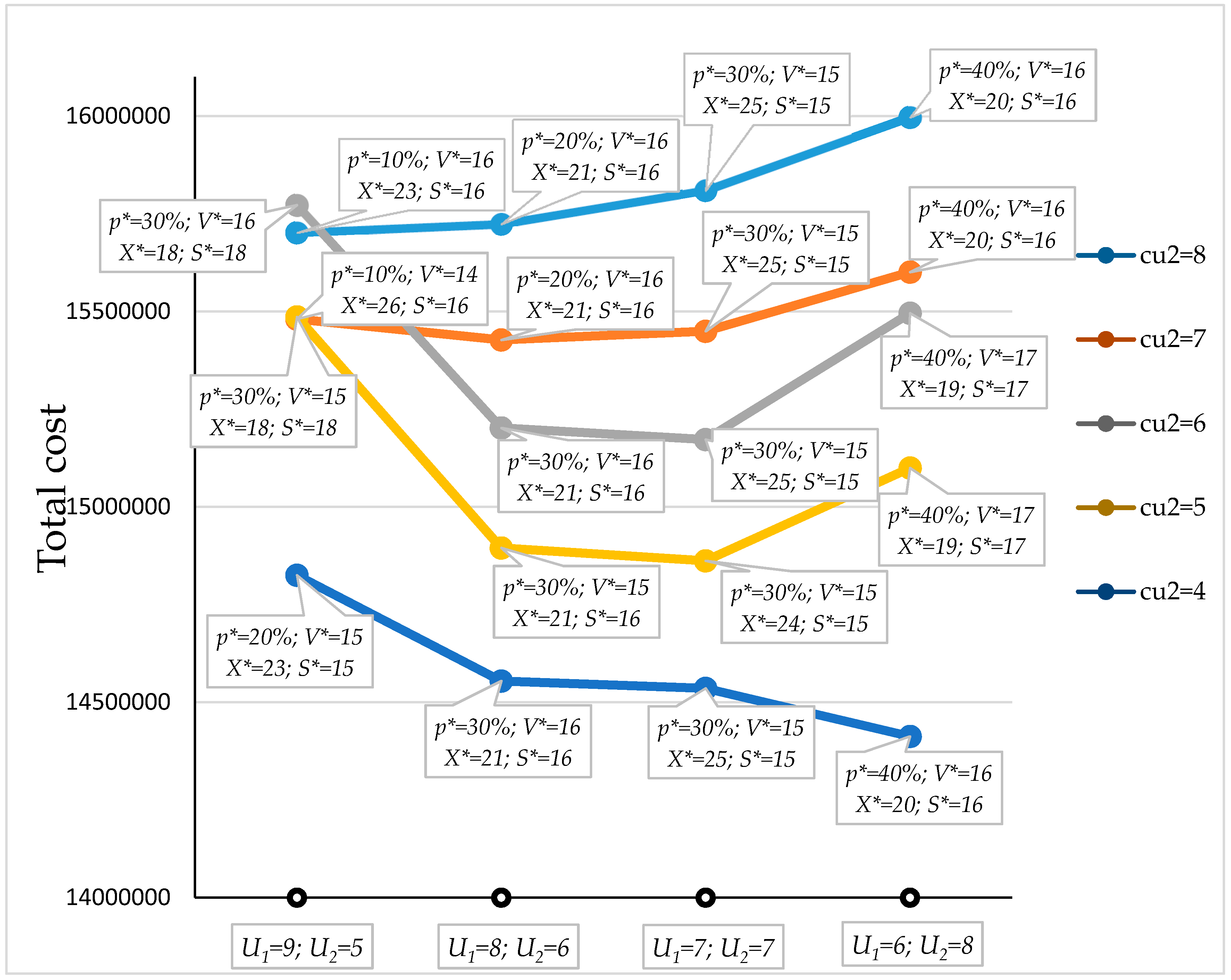
The results can be seen in Figure 7.
In Figure 7, we can see that the higher cu2 is, the more the production goes to manufacturing on M1 and vice versa. This is logical, because, when the unit remanufacturing cost increases, remanufactured product will have a cost near to those of a manufactured one. Indeed, for the remanufactured product, we have the remanufacturing cost, the inventory recovery cost and the return cost. In this study, we can also determine the optimal configuration and optimal values p*, S*, V* and X* according to the unit remanufacturing cost. For example, when cu2 = 6, the optimal configuration is when U1 = 7 and U2 = 7 and also when p* = 30%, V* = 15, X* = 25 and S* = 15. This study allows for any company leader to find in the same time optimal machines configuration, optimal values of return of the used products, manufacturing stock, purchasing warehouse and vehicle capacities.
5. Conclusions
In this paper, a manufacturing–remanufacturing–transport–warehousing closed-loop supply chain is considered. The proposed system is composed of two machines for manufacturing and remanufacturing, manufacturing stock, purchasing warehouse, transport vehicle and recovery inventory. The vehicle transports the products from the manufacturing stock to the purchasing warehouse. Customers demand is constant and is supposed to be lost when it is unsatisfied. We also considered that the returned amount of used end-of-life products was based on the sales of the past periods, and not on the demand. A hedging point policy is defined to control manufacturing and remanufacturing, with preserving the coordination between manufacturing, remanufacturing, inventorying and return of end-of-life products. Discrete flow model is proposed to faithfully describe the system and to formulate the problem. Total cost function program was encoded with the C++. Since the model is stochastic, we had to set a high value of total simulation time and to repeat simulation several times in order to obtain more accurate results. In such a case, simulation is extremely time consuming and this is why we applied genetic algorithm, which allowed us to dramatically cut down the duration of optimization. The optimization program determines optimal values of manufacturing stock, vehicle and purchasing warehouse capacities and optimal return of used products. Finally, we illustrated the performance of our model by numerical examples, and we have shown how the optimal values of decision variables depend on different model indicators, such as transportation time, unit remanufacturing cost and manufacturing/remanufacturing machines configuration.
In future works, we will consider a more complex system with random demand and random return of used end-of-life products.
Acknowledgments
This research was supported by the Industrial Engineering and Production Laboratory of Metz (France).
Author Contributions
Sadok Turki is the responsible for conducting this research. He proposed the main paper contribution and developed the mathematical model and the simulation program. Stanislav Didukh contributed to writing of the paper and results analysis. Christophe Sauvey contributed to propose and to develop the optimization method. Nidhal Rezg supervised this work and contributed to revise this paper.
Conflicts of Interest
The authors declare no conflict of interest.
References
- Galve, J.E.; Elduque, D.; Pina, C.; Javierre, C. Sustainable supply chain management: The influence of disposal scenarios on the environmental impact of a 2400 L waste container. Sustainability 2016, 8, 564. [Google Scholar] [CrossRef]
- Moon, I.; Jeong, Y.J.; Saha, S. Fuzzy Bi-Objective Production-Distribution Planning Problem under the Carbon Emission Constraint. Sustainability 2016, 8, 798. [Google Scholar] [CrossRef]
- Despeisse, M.; Ball, P.D.; Evans, S.; Levers, A. Industrial ecology at factory level—A conceptual model. J. Clean. Prod. 2012, 31, 30–39. [Google Scholar] [CrossRef]
- Liu, C.; Yang, J.; Lian, J.; Li, W.; Evans, S.; Yin, Y. Sustainable performance oriented operational decision-making of single machine systems with deterministic product arrival time. J. Clean. Prod. 2014, 85, 318–330. [Google Scholar] [CrossRef]
- Li, J.; Du, W.; Yang, F.; Hua, G. The carbon subsidy analysis in remanufacturing closed-loop supply chain. Sustainability 2014, 6, 3861–3877. [Google Scholar] [CrossRef]
- Van Nunen, A.E.E.J.; Zuidwijk, R.A. E-enabled closed-loop supply chains. Calif. Manag. Rev. 2004, 46, 40–54. [Google Scholar] [CrossRef]
- Salema, M.I.G.; Povoa, A.P.B.; Novais, A.Q. An Optimization Model for the Design of a Capacitated Multi-Product Reverse Logistics Network with Uncertainty. Eur. J. Oper. Res. 2007, 179, 1063–1077. [Google Scholar] [CrossRef]
- De Brito, M.P.; Dekker, R.; Flapper, S.D.P. Reverse Logistics—A Review of Case Studies; Report Series Research in Management, ERS-2003-012-LIS; Erasmus Research Institute of Management: Berlin, Germany, 2003. [Google Scholar]
- Guide, V.D.R., Jr.; Van Wassenhove, L.N. OR FORUM—The evolution of closed-loop supply chain research. Oper. Res. 2009, 57, 10–18. [Google Scholar] [CrossRef]
- Mitra, S. Inventory management in a two-echelon closed-loop supply chain with correlated demands and returns. Comput. Ind. Eng. 2012, 62, 870–879. [Google Scholar] [CrossRef]
- Kenne, J.P.; Dejax, P.; Gharbi, A. Production planning of a hybrid manufacturing–remanufacturing system under uncertainty within a closed-loop supply chain. Int. J. Prod. Econ. 2012, 135, 81–93. [Google Scholar] [CrossRef]
- Chung, S.L.; Wee, H.M.; Yang, P.C. Optimal Policy for a Closed-Loop Supply Chain Inventory System with Remanufacturing. Math. Comput. Model. 2008, 48, 867–881. [Google Scholar] [CrossRef]
- Turki, S.; Hajej, Z.; Rezg, N. Performance Evaluation of a Hybrid Manufacturing Remanufacturing System Taking Into Account the Machine Degradation. In Proceedings of the 15th IFAC Symposium on Information Control Problems in Manufacturing (INCOM 15), Ottawa, ON, Canada, 11–13 May 2015. [Google Scholar]
- Turki, S.; Rezg, N. Unreliable manufacturing supply chain optimisation based on an infinitesimal perturbation analysis. Int. J. Syst. Sci. Oper. Logist. 2016. [Google Scholar] [CrossRef]
- Turki, S.; Hennequin, S.; Sauer, N. Performances evaluation of a failure-prone manufacturing system with time to delivery and stochastic demand. In Proceedings of the 13th IFAC Symposium on Information Control Problems in Manufacturing (INCOM 09), Moscow, Russia, 3–5 June 2009; Volume 13. [Google Scholar]
- Teunter, R.H. Economic ordering quantities for recoverable item inventory systems. Nav. Res. Logist. 2001, 48, 484–495. [Google Scholar] [CrossRef]
- Tang, O.; Grubbström, R.W. The detailed coordination problem in a two-level assembly system with stochastic lead times. Int. J. Prod. Econ. 2003, 81, 415–429. [Google Scholar] [CrossRef]
- Tang, O.; Grubbström, R.W. Considering stochastic lead times in a manufacturing/remanufacturing system with deterministic demands and returns. Int. J. Prod. Econ. 2005, 93, 285–300. [Google Scholar] [CrossRef]
- Darla, S.P.; Naiju, C.D.; Annamalai, K.; Sravan, Y.U. Production and Remanufacturing of Returned Products in Supply Chain using Modified Genetic Algorithm. World Acad. Sci. Eng. Technol. Int. J. Mech. Aerosp. Ind. Mechatron. Manuf. Eng. 2012, 6, 574–577. [Google Scholar]
- Kelle, P.; Silver, E.A. Purchasing Policy of New Containers Considering the Random Returns of Previously Issued Containers. IIE Trans. 1989, 21, 349–354. [Google Scholar] [CrossRef]
- Toktay, L.B.; Wein, L.M.; Zenios, S.A. Inventory management of remanufacturable products. Manag. Sci. 2000, 46, 1412–1426. [Google Scholar] [CrossRef]
- Sadok, T.; Nidhal, R. Perturbation analysis for discrete flow model: Optimization of a manufacturing-remanufacturing system. In Proceedings of the 2014 IEEE International Conference on Systems, Man and Cybernetics (SMC), San Diego, CA, USA, 5–8 October 2014; pp. 2569–2574. [Google Scholar]
- Yao, C.; Cassandras, C.G. Using infinitesimal perturbation analysis of stochastic flow models to recover performance sensitivity estimates of discrete event systems. Discret. Event Dyn. Syst. 2012, 22, 197–219. [Google Scholar] [CrossRef]
- Xie, X.; Hennequin, S.; Mourani, I. Perturbation analysis and optimisation of continuous flow transfer lines with delay. Int. J. Prod. Econ. 2013, 51, 7250–7269. [Google Scholar] [CrossRef]
- Mourani, I.; Hennequin, S.; Xie, X. Simulation-based optimization of a single-stage failure-prone manufacturing system with transportation delay. Int. J. Prod. Econ. 2008, 112, 26–36. [Google Scholar] [CrossRef]
- Falkenauer, E. A hybrid grouping genetic algorithm for bin packing. J. Heuristics 1996, 2, 5–30. [Google Scholar] [CrossRef]
- Rubinowitz, J.; Levitin, G. Genetic algorithm for assembly line balancing. Int. J. Prod. Econ. 1995, 41, 343–354. [Google Scholar] [CrossRef]
- Akella, R.; Kummar, P.R. Optimal control of production rate in failure prone manufacturing system. IEEE Trans. Autom. Control 1986, 31, 116–126. [Google Scholar] [CrossRef]
- Lia, Y.; Yub, J.; Ta, D. Genetic algorithm for spanning tree construction in P2P distributed interactive applications. Neurocomputing 2014, 140, 185–192. [Google Scholar] [CrossRef]
- Lasheen, M.; Abdel Rahman, A.K.; Abdel-Salam, M.; Ookawara, S. Performance enhancement of constant voltage based MPPT for photovoltaic applications using genetic algorithm. Energy Procedia 2016, 100, 217–222. [Google Scholar] [CrossRef]
- Cornejo-Bueno, L.; Nieto-Borge, J.C.; Garcia-Diaz, P.; Rodriguez, G.; Salcedo-Sanz, S. Significant wave height and energy flux prediction for marine energy applications: A grouping genetic algorithm—Extreme Learning Machine approach. Renew. Energy 2016, 97, 380–389. [Google Scholar] [CrossRef]
- Sauvey, C.; Sauer, N. A genetic algorithm with genes-association recognition for flowshop scheduling problems. J. Intell. Manuf. 2012, 23, 1167–1177. [Google Scholar] [CrossRef]
Figure 1.
Manufacturing–remanufacturing–transport–warehousing closed-loop supply chain.

Figure 2.
Studied time horizon.

Figure 3.
Example of the transport from B to W.

Figure 4.
Frequency of transportation and customers’ demands throughout the time horizon.
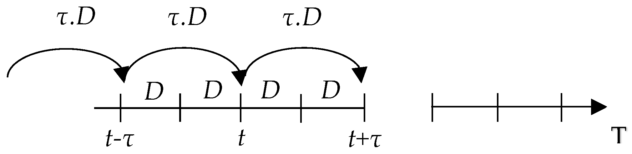
Figure 5.
Products’ service life.
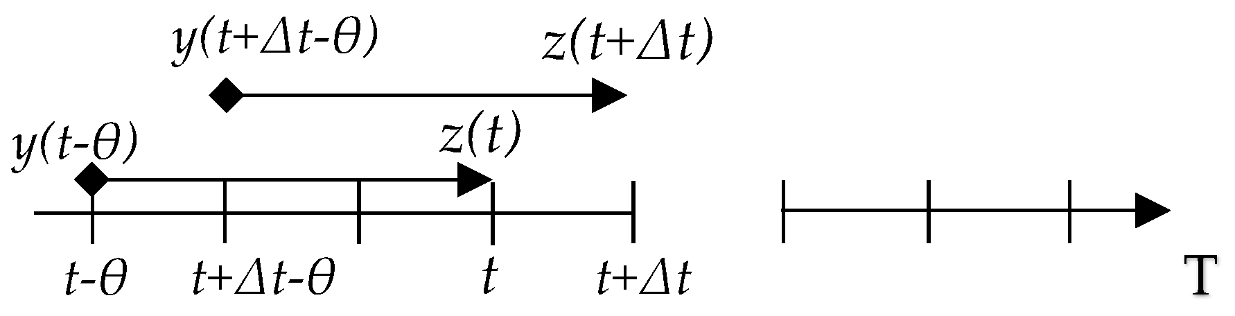
Figure 6.
(a) Production control illustration; and (b) production control illustration.

Figure 7.
Influence of the unit manufacturing/remanufacturing costs on the optimal machines configuration.
Figure 7.
Influence of the unit manufacturing/remanufacturing costs on the optimal machines configuration.


Table 1.
Influence of returned used end-of-life products (p) relative percentage to the sales on S*, V* and X*.
Table 1.
Influence of returned used end-of-life products (p) relative percentage to the sales on S*, V* and X*.
| p | S* | V* | X* | F(T) |
|---|---|---|---|---|
| 10% | 16 | 15 | 27 | 15,022,529 |
| 20% | 15 | 15 | 23 | 14,824,557 |
| 30% | 15 | 14 | 19 | 15,148,097 |
| 40% | 14 | 13 | 17 | 41,847,037 |
| 50% | 11 | 11 | 11 | 214,821,535 |
Table 2.
Influence of the value of τ (transportation time) on p*, S*, V* and X*.
| τ | p* | S* | V* | X* | F(T) | τ·d | X*/(τ·d) |
|---|---|---|---|---|---|---|---|
| 1 | 20% | 15 | 15 | 23 | 14,824,557 | 10 | 2.3 |
| 2 | 30% | 29 | 29 | 29 | 18,562,953 | 20 | 1.45 |
| 3 | 30% | 38 | 38 | 38 | 21,981,917 | 30 | 1.27 |
| 4 | 30% | 48 | 48 | 48 | 25,292,159 | 40 | 1.20 |
| 5 | 30% | 58 | 58 | 58 | 28,251,540 | 50 | 1.16 |
| 6 | 30% | 68 | 68 | 68 | 31,413,165 | 60 | 1.13 |
| 7 | 30% | 77 | 77 | 77 | 34,594,556 | 70 | 1.10 |
| 8 | 30% | 86 | 86 | 86 | 37,115,528 | 80 | 1.07 |
| 9 | 30% | 96 | 96 | 96 | 40,614,008 | 90 | 1.06 |
| 10 | 30% | 104 | 104 | 104 | 43,707,006 | 100 | 1.04 |
Table 3.
Study of the influence of inventory holding costs on the system’s outcomes.
| cs | cw | τ | P* | S* | V* | X* | F(T) |
|---|---|---|---|---|---|---|---|
| 1 | 4 | 4 | 30% | 66 | 40 | 56 | 27,729,534 |
| 4 | 1 | 4 | 20% | 46 | 46 | 65 | 26,453,331 |
Table 4.
Influence of machines reconfiguration on the vector p*, S*, V* and X*.
| U1 | U2 | cu1 | cu2 | P* | V* | X* | S* | COST |
|---|---|---|---|---|---|---|---|---|
| 9 | 5 | 10 | 4 | 20% | 15 | 23 | 15 | 14,824,557 |
| 8 | 6 | 10 | 4 | 30% | 16 | 21 | 16 | 14,553,720 |
| 7 | 7 | 10 | 4 | 30% | 15 | 25 | 15 | 14,535,097 |
| 6 | 8 | 10 | 4 | 40% | 16 | 20 | 16 | 14,411,959 |
© 2017 by the authors. Licensee MDPI, Basel, Switzerland. This article is an open access article distributed under the terms and conditions of the Creative Commons Attribution (CC BY) license (http://creativecommons.org/licenses/by/4.0/).
Share and Cite
MDPI and ACS Style
Turki, S.; Didukh, S.; Sauvey, C.; Rezg, N. Optimization and Analysis of a Manufacturing–Remanufacturing–Transport–Warehousing System within a Closed-Loop Supply Chain. Sustainability 2017, 9, 561. https://doi.org/10.3390/su9040561
AMA Style
Turki S, Didukh S, Sauvey C, Rezg N. Optimization and Analysis of a Manufacturing–Remanufacturing–Transport–Warehousing System within a Closed-Loop Supply Chain. Sustainability. 2017; 9(4):561. https://doi.org/10.3390/su9040561
Chicago/Turabian StyleTurki, Sadok, Stanislav Didukh, Christophe Sauvey, and Nidhal Rezg. 2017. "Optimization and Analysis of a Manufacturing–Remanufacturing–Transport–Warehousing System within a Closed-Loop Supply Chain" Sustainability 9, no. 4: 561. https://doi.org/10.3390/su9040561
Note that from the first issue of 2016, this journal uses article numbers instead of page numbers. See further details here.