Article

Mortality Associated with High Ambient Temperatures, Heatwaves, and the Urban Heat Island in Athens, Greece

by
John Paravantis
1,
Mat Santamouris
2,
Constantinos Cartalis
3,*,
Chrysanthi Efthymiou
3 and
Nikoletta Kontoulis
1
1
Department of International and European Studies, University of Piraeus, Piraeus 185 34, Greece
2
The Anitta Lawrence Chair of High Performance Architecture, Faculty of Built Environment, University of New South Wales, Sydney, NSW 2052, Australia
3
Department of Environmental Physics, National and Kapodistrian University of Athens, Athens 157 72, Greece
*
Author to whom correspondence should be addressed.
Sustainability 2017, 9(4), 606; https://doi.org/10.3390/su9040606
Submission received: 23 November 2016 / Revised: 29 March 2017 / Accepted: 11 April 2017 / Published: 13 April 2017
(This article belongs to the Special Issue Urban Heat Island)

Abstract

:
Climate change looms as the biggest threat of the 21st century, and its effect on urban mortality is exacerbated by urban heat islands. This study analyzes the impact of high temperatures, heatwaves, and the urban heat island on the cardiovascular and respiratory mortality of people over 65 years of age for the years 2002 to 2012. The area of application is Athens, Greece, an urban agglomeration experiencing an urban heat island of high intensity. The correlation of the daily cardiovascular and respiratory mortality count of people over 65 years of age with various temperature measures confirmed a U-shaped exposure response curve, with fewer deaths in the range of moderate temperatures. At high and very high temperatures, this mortality increased by 20% to 35% correspondingly, at a 99.9% significance level. Mortality was further investigated with ordinary least squares, Poisson, and negative binomial times series models, which, although suffering from poor fit, showed a one-day lag for the maximum temperature effect on mortality. Finally, cluster analysis for observations confined to May to September, confirmed by multiple discriminant analysis, showed the existence of six clusters, with the highest excess mortality count of 23% for the cluster that included the hottest days and 20.6% for the heatwave cluster. To this end, it is recommended that policies target high ambient temperatures and heatwaves as a priority.

1. Introduction

Climate change may well constitute the biggest global health threat of the 21st century [1,2]. The negative impact of global warming is exacerbated by the urban heat island (UHI) phenomenon, which refers to cities being hotter than surrounding rural areas, affecting people in urban areas in ways worse than mild thermal discomfort [3]. The UHI refers to the development of high ambient air temperatures in the dense part of cities compared to surrounding suburban or rural areas. Higher urban ambient temperatures are the result of the positive urban thermal balance that is highly controlled by the increased absorption of shortwave radiation and the excessive release of anthropogenic heat.
Data on the amplitude of the urban heat are available for more than 400 cities around the world, and the average urban heat island intensity exceeds 5–6 °C [4,5]. The UHI and the local climate change affect the environmental quality of cities highly as they increase the energy spent for cooling purposes [6], increase the peak electricity demand during the summer period [7], deteriorate thermal comfort conditions [8], and increase the thermal stress to low income and vulnerable segments of the population [9]. The UHI is enhanced during heatwaves, as the difference between urban and rural temperatures is increased because of higher ambient temperatures, especially during the night. Given the impact of increased urbanization on the intensity of the urban heat island and that heatwaves are projected to become more frequent due to climate change, heat-related health risks for urban residents are expected to worsen in the twenty-first century. Adaptation and mitigation strategies will require, among others, more reflective materials and more green and blue spaces.
The urban heat island and global climate change affect the urban climate, but their specific impact may not always act in a synergistic way. However, most studies conclude that the UHI increases considerably during heatwave periods [10,11]. Urban air pollution is implicated as well since the adverse effects of the UHI include an elevation in the concentration of ground-level ozone [12] and an increase in mortality [13]. High ambient temperatures in urban areas relate to serious medical problems, affecting vulnerable groups including the elderly and individuals suffering from cardiovascular or respiratory diseases [14]. During heatwaves, especially in temperate latitudes, the UHI intensifies heat stress, particularly at night [15]. Robine et al. [16] collected the daily number of regional deaths in 16 European countries, analyzed the summer mortality for 1998–2002 (considered the reference period) and for 2003, and concluded that more than 70,000 additional deaths occurred in Europe during the summer of 2003, when a European-wide heatwave hit.
Extreme temperatures are a cause of mortality [17] and the leading cause of weather-related mortality [18]. It has also been established that the increase in winter and summer mortality is indirectly [19] attributed to cardiovascular and respiratory causes, especially in the elderly [20]. Exposure of the population to high ambient temperatures has a significantly negative impact on health and increases mortality rates [21], rapidly over a threshold temperature, which appears to be higher in the Mediterranean countries, 29.4 °C, compared to northern and continental European areas, where it equals 23.3 °C [22]. Heatwaves amplify heat-related mortality [23], especially in the elderly, so some studies have focused on the mortality of people over 65 years of age [24,25]. Such heat-related mortality in urban areas, being more of a risk to the elderly and those with chronic cardiorespiratory disease, is likely to be intensified in the coming decades by the effects of global warming [26] and the augmentation of UHIs.
The goal of this research is to carry out an analysis of the association of high temperatures with heatwaves and consecutively to enhanced UHI and urban air pollution to the cardiovascular and respiratory mortality of people over 65 years of age. The goals also include the comparison of the impact of high and low ambient temperatures on mortality, to shed light on the enhanced importance of the effects of high urban temperatures in areas that are characterized by a UHI. The paper is structured as follows: a literature review (Section 1.1) and methods (Section 2) are followed by an analysis of temperature, humidity (Section 3.1), and air pollution (Section 3.2). Fatalities due to cardiovascular and respiratory causes in individuals over 65 years of age are examined in Section 3.3, with estimates of functional forms and tests of statistical significance. Section 3.4 carries out a cluster analysis, which is confirmed by a discriminant analysis. Finally, the manuscript ends with a discussion (Section 4).

1.1. Literature Review

In a study of the correlation between temperature and cardiovascular or respiratory mortality of the elderly in the 20 largest metropolitan areas in the USA, Basu, Dominici, and Samet [27] estimated comparable epidemiological time series (conditional logistic and Poisson regression) models and established that the strongest association was found in the summer. The authors point out that heat-related deaths are likely underreported because some may be attributed to other causes. The mean daily and dew-point daily temperatures were used in the analysis, which considered the confounding effect of air pollution (particulate matter and ozone) and did not exclude nonresident deaths, arguing that temperature is thought to have an acute response. Although the authors used data from only one year (1992), they found their models to be in strong agreement (with slight variations in consistency) about season and geographic region, in showing that elevated cardiovascular and respiratory mortality were associated with temperature exposure mostly in the summer.
Harlan et al. [28] researched the mortality of males and females over and under 65 years of age during the summer months (i.e., the months May to October of the years 2000 to 2008) in desert cities of central Arizona that have an extremely hot climate. Cubic spline regressions were estimated, to describe the relationship between temperature and mortality, using dummy variables for heatwave days and their lags (up to three days); day of the week and holiday dummies were not found to be significant. Among the causes of death examined were: direct exposure to environmental heat, dehydration, cardiac disease or stroke, heart failure, chronic obstructive pulmonary disease and asthma, other respiratory diseases, and chronic renal failure. All groups, except males over 65 years of age, were found to have an elevated relative risk of death from all causes, with one-day lag effects. The authors found increasing mortality above threshold temperature values for direct exposure to environmental heat. Moreover, temperature effects on direct heat exposure deaths were found to be statistically significant for all age and gender groups. The daily maximum apparent temperature was found to be more robustly associated with mortality from direct exposure to high ambient heat.
In a study of mortality during a heatwave (May 2010) in Ahmedabad, India, Azhar et al. [19] analyzed death counts for 2010 using seven-day moving averages, mortality rate ratios, and the daily maximum temperature. The period of the heatwave was found to be characterized by a very significant excess of mortality (43.1% increase over a reference period), with no lag time observed between temperatures and fatalities. Moderate to high correlations were found between mortality and temperature (particularly when the maximum temperature was over 43 °C and the mean temperature over 36 °C) in the hot summer months of April, May, and June, with significantly more female deaths in these summer months and the heatwave period. No cause-specific analysis of deaths was performed.

Heat Mortality in Europe

In terms of research studies focusing on mortality in Europe, Baccini et al. [22] examined the association between daily maximum apparent temperature and daily deaths during the warm season (April to September, with the study period ranging from five to 11 years around 1990–2000) in 15 European cities (including Athens, Greece) with six other Mediterranean cities (Barcelona, Ljubljana, Milan, Rome, Turin, and Valencia) and nine northern continental cities (Budapest, Dublin, Helsinki, London, Paris, Prague, Stockholm, and Zurich). Among others, the aim of this research was to explore the delayed effect of heat and test the assumption of a constant heat effect over the summer period. Mortality counts were subdivided by age groups (15 to 64, 65 to 74, and over 75 years of age), with data available for cardiovascular and respiratory fatalities separately. The effects of heat and cold were examined separately. Confounding variables included air pollution (represented, as a proxy, by nitrogen dioxide concentration), wind speed, barometric pressure, month, day of the week, holidays as well as linear and quadratic trend variables. Lags of up to 40 days for the maximum apparent temperature were considered to account even for delayed effects of exposure to extreme temperatures. The authors confirmed that the exposure–response curves that depict the association between maximum and minimum apparent temperature and log mortality are J-shaped (or U-shaped), with the lowest mortality appearing at a range of moderate temperature values and rising progressively as temperatures increase or decrease. Plotting the data for Mediterranean and northern continental cities separately showed that the effect of maximum apparent temperature was somewhat stronger for Mediterranean cities. Heat effects were reported as percent changes in the mortality associated with a 1 °C increase in the maximum apparent temperature above a city-specific threshold (lower for northern continental cities, implying an increased susceptibility of their residents at lower values of apparent temperature), which for Athens equaled 32.7 °C (with a 95% confidence interval spanning 32.1–33.3 °C). Finally, the authors found stronger associations between heat and mortality from respiratory diseases, and with mortality from all causes for ages above 75 years, with heterogeneity observed among cities, especially those in the Mediterranean.
Heat-related mortality peaks during heatwaves, which are often defined as spells of consecutive days with maximum temperatures exceeding the 90th percentile of the 1961–1990 period; these have also been defined as periods of at least two days [29] that have unusually and excessively hot weather, usually accompanied by high humidity [19]. The impact of summer heatwaves on the mortality of people over 65 years of age was examined by D’Ippoliti et al. [24]. Heatwaves in nine European cities, including Athens along with four other Mediterranean cities (Barcelona, Milan, Rome, and Valencia) and four continental cities (Budapest, London, Munich, and Paris), were defined by the maximum apparent as well as the minimum temperature (flagging hot nights) and were classified by intensity, duration, and timing (for the months of June, July, and August). Gender, age, and cause of death were considered in the analysis of daily mortality counts. Great geographical heterogeneity among the cities was found, with Mediterranean cities characterized by a greater impact of temperature extremes. Potential confounding variables considered included day of the week, calendar month, barometric pressure (including time lags), wind speed, and the concentration of nitrogen dioxide. Data for Athens spanned 1997 to 2004, with the summer of 2003 marking one of the worst European heatwaves in recent history. Cerebrovascular mortality during heatwaves was highest in Athens (17.7% of total fatalities), with the highest effect found for fatalities caused by respiratory diseases in females aged 75–84.
The association of daily mortality with thermal conditions (in both hot and cold weather) in Athens (1992–2001) was also researched by Nastos and Matzarakis [30]. Daily maximum and minimum temperatures were considered, along with the daily values of two indexes intended to assess physiological thermal stress. Statistical analysis showed significant correlations among daily temperature, thermal indexes, and mortality, with a one-day lag also having a significant effect on hot-weather mortality. These authors cite various studies (in different countries) that support the widely-established notion of daily mortality being a U-shaped function of temperature, with the mortality at a minimum at a value varying from 16.5 to 24 °C (with northern regions generally having lower temperatures) and rising below and above this point. It was found that a daily minimum temperature greater than 23.4 °C seemed to quadruple the mortality risk, while a daily maximum temperature greater than 33 °C seems to multiply the mortality risk by a factor of six. The U-shaped (quadratic) form of the relationship between (minimum, maximum, and index) temperature and mortality was confirmed, with cold weather also affecting mortality in a way that was as important as that attributed to heat for specific types of deaths [31].
Heatwaves are expected to become more frequent and severe during the 21st century as global warming intensifies [32,33,34]. Referring to the Iberian Peninsula and the Mediterranean region, Fischer and Schar [35] assert that the frequency of heatwave days will increase, from an average of about two days per summer for the period 1961–1990 to around 13 days for 2021–2050 and 40 days for 2071–2100, expecting the urban areas of Athens, Bucharest, Marseille, Milan, Rome, and Naples to experience the greatest health effects. They consider warm nights to exacerbate health effects, by causing sleep deprivation and inhibiting recovery from daytime heat. They also note that relative humidity, an important thermoregulation factor, is a stress factor when combined with high temperatures, as the evaporation rate of sweat is reduced.
Researching heatwaves that have been observed in Greece since 1951, Papanastasiou, Melas, and Kambezidis [36] considered a heatwave to have occurred when the daily maximum temperature is at least 37 °C and the daily average temperature is at least 31 °C in a city center. While few heatwave days were identified until the mid-1960s and no heatwave days were identified during in the early 1990s, an increasing trend seems to be in effect since 1992, with the most prolonged heatwave ever recorded in a 12-day event observed in 2010 [36,37].

2. Materials and Methods

To establish an association between mortality and high temperatures (associated with UHI and heatwaves), this research analyzed the fatalities that occurred in the municipality of Athens. A total of 36,038 daily death counts were made available to this research by the Hellenic Statistical Authority, for the period 1 January 2002–31 December 2012. Counts included the total number of daily deaths (for the entire city of Athens) per gender, age group, and cause of death. In addition, meteorological data were obtained from the meteorological station of the National Observatory of Athens. Temperature and humidity data from the Patission Street monitoring station were selected because it is located on a major street in central Athens and had few missing values.
The following variables were available for each observation:
  • year, date, and day of the week;
  • minimum and maximum temperature and apparent temperature (°C);
  • minimum and maximum relative humidity (%);
  • gender of deceased individuals;
  • age group of deceased individuals (in classes of five-year width);
  • cause of death (categories shown in Table 1); number of daily deaths per gender, age group, and cause.
The variable names employed are presented in the list of abbreviations at the end of this paper.
Heatwaves were defined per the criteria set by the Hellenic National Meteorological Service, i.e., at least three consecutive days with maximum air temperature higher or equal to 36.5 °C [38]. Furthermore, motivated by the work of Robine et al. [16], who found no harvesting effect in the months following the pan-European heatwave of 2003, it was decided that harvesting (i.e., the compensatory reduction in overall mortality in the weeks after a heatwave) would not be accounted for in this research. Also, the use of a heatwave days variable allowed for considering the number of consecutive days in a heatwave.
Following a descriptive analysis of temperature and humidity, an analysis of mortality was carried out, including the estimation of exposure–response curves between mortality and temperature (Section 3.2). Next, time series models were estimated, appropriate for the count of daily fatalities below 65 years of age that were attributed to cardiovascular or respiratory causes (Section 3.3). Finally, cluster analysis was run on mortality, temperature, and humidity data, with a discriminant analysis employed to confirm the chosen clustering scheme (Section 3.4).
Graphing was done with Minitab (version 17) (Minitab Inc., Pennsylvania, PA, USA), while statistical analyses were done with Minitab (version 17), SPSS (version 23) (IBM Corp., Armonk, NY, USA), the 2016d version of the Gretl regression, econometric and time-series library [39], and Stata (version 13) (StataCorp, College Station, TX, USA).

3. Results

3.1. Temperature and Humidity

The maximum daily temperature (TEMPMAX) for the entire study period ranged from −1.82 to 43.80 °C, with a mean of 22.80 °C, while the maximum apparent temperature ranged from 1.53 to 48.51 °C with a mean of 24.45 °C (the apparent temperature is a metric of how hot it feels to people when air temperature, wind, and relative humidity are considered [29]). The distribution of the maximum temperature showed three modes, at around 17, 28, and 34 °C. The distribution of the maximum apparent temperature appeared to have two modes, at around 18 and 35 °C. The minimum daily temperature (TEMPMIN) for the entire study period ranged from −5 to 31.09 °C, with a mean value of 15.37 °C. The distribution of the minimum temperature had three modes (peaks), around 12, 18, and 26 °C, possibly corresponding to the prevailing weather conditions during the winter, the spring/summer, and the autumn months, respectively. The minimum apparent temperature ranged from −6.96 to 36.98 °C with a mean of 16.91 °C.
The minimum daily humidity (RELHUMIN) for the entire study period ranged from 8% to 91% with a mean of 47.14%, while the maximum humidity (RELHUMAX) ranged from 32% to 101% with a mean of 77.16%. While the minimum humidity followed a symmetric (nearly normal) distribution within its range of values, the maximum humidity displayed a strong negative skewness, with many values in the range of 80%–90%. It is noted that humidity is considered in the calculation of the apparent temperature.
The variation of average minimum and maximum values of temperature and humidity per month confirmed the expected seasonal variability, with higher temperature and lower humidity values during the summer months.
Finally, using the definition of heatwaves mentioned in the materials and methods section, 2012, 2007, and 2010 were the years with the highest number of heatwaves (20, 10, and 8, respectively), while 2003 (the year of the European heatwave) was only characterized by two short heatwaves in Greece. Of the other years of the sample, 2005 and 2006 had four heatwaves; 2004, 2009, and 2011 had one heatwave; and 2002 and 2008 had zero heatwaves.

3.2. Mortality

Following the examination of temperature and humidity, attention now shifts to the fatalities that occurred in the municipality of Athens during the period considered in this research (2002–2012). The number of deaths (mortality count) rather than the proportion of deaths in the population (mortality rate) was analyzed; the concept of excess mortality is discussed in the discussion section.
In the years 2002 to 2012, a total of 89,658 fatalities occurred due to various causes. Of these, 51.4% were female and 48.6% were male. The mean age of death from all causes was 75.6 years (72.2 for males; 78.7 for females). The distribution of total fatalities per month of the year confirmed a connection to temperature extremes: the highest mortality counts occurred in the months of December to March and July to August. Regarding the day of the week, there was a slight variation, with more fatalities occurring on Monday and fewer during the weekend (Saturday and Sunday).
A closer examination of the cause of death, shown in Table 1, shows that cardiovascular disease, cancers, and respiratory diseases were the most frequent cause of death, jointly responsible for almost eight out of 10 deaths (78.3%) for the duration of the research.
The breakdown of fatalities by year and cause (not shown) did not reveal any significant annual changes in the distribution of deaths among the different causes for the period under study. The distribution of fatalities from different causes per month (also not shown) confirms the correlation between cardiovascular and respiratory deaths and the time of year (more in the coldest winter and hottest summer months).
The rest of this research now focuses on the deaths of individuals over 65 years of age that were due to cardiovascular and respiratory causes; these have been examined in the epidemiological research literature (e.g., [
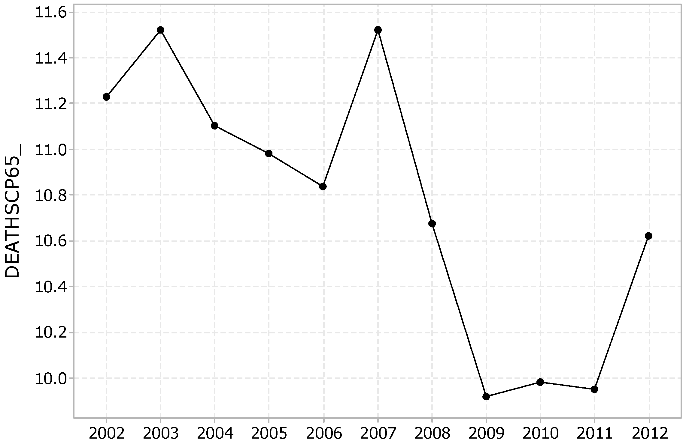
27]) as potentially attributed to temperature extremes. The total number of such fatalities was 4018 out of a total of 89,658 (4.5%). The daily average number of such deaths was equal to 10.761, with a minimum of one and a maximum of 33 deaths. The distribution of cardiovascular and respiratory fatalities of individuals over 65 years per day (i.e., the daily mortality count), follows a relatively symmetric distribution with a slight positive skew. Regarding the average annual variation of cardiovascular and respiratory fatalities of people over 65 years of age, as shown in Figure 1, it is observed that such fatalities were exacerbated in 2003, the year of a pan-European heatwave [16] and 2007, and appeared to have a minimum in the years 2009, 2010, and 2011.
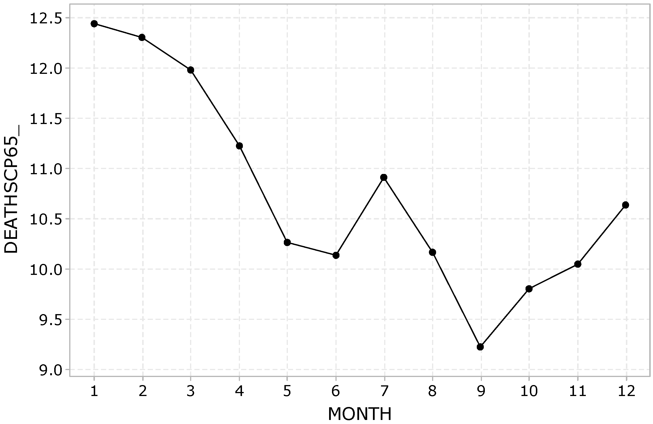
Regarding the average monthly variation of cardiovascular and respiratory deaths of people over 65 years of age, as shown in Figure 2, these showed an upsurge in the winter months, a decline during the spring and the autumn, and a smaller peak in the middle of summer, with the lowest value occurring in September.
Of particular interest in the literature is the correlation of the daily number of cardiovascular and respiratory deaths of individuals over 65 years of age, to the daily maximum (apparent) temperature. The functional form of some such exposure response curves, fit as quadratic equations via ordinary least squares, are shown in Equations (1)–(4).
Equations (1) and (2) show the functional form of the association between the daily mortality count of cardiovascular and respiratory deaths of individuals over 65 years of age and maximum temperature, in both raw and logarithmic form.
DEATHSCP65_ = 15.17 − 0.3720 TEMPMAX + 0.006882 TEMPMAX2
log10(DEATHSCP65_) = 1.188 − 0.01562 TEMPMAX + 0.000289 TEMPMAX2
where DEATHSCP65_ is the daily fatality count below 65 years of age attributed to cardiovascular or respiratory causes, and TEMPMAX is the daily maximum temperature (measured in °C).
Equations (3) and (4) show the functional form of the association between the daily mortality count of cardiovascular and respiratory deaths of individuals over 65 years of age and maximum apparent temperature, also in both raw and logarithmic form:
DEATHSCP65_ = 14.14 − 0.2609 APPTEMPMAX + 0.004364 APPTEMPMAX2
log10(DEATHSCP65_) = 1.146 − 0.01104 APPTEMPMAX + 0.000185 APPTEMPMAX2
where DEATHSCP65_ is the daily fatality count below 65 years of age attributed to cardiovascular or respiratory causes, and APPTEMPMAX is the daily maximum apparent temperature (measured in °C).
The maximum temperature is regarded as the most representative [30]. As an illustration of the functional form of the above equations, 
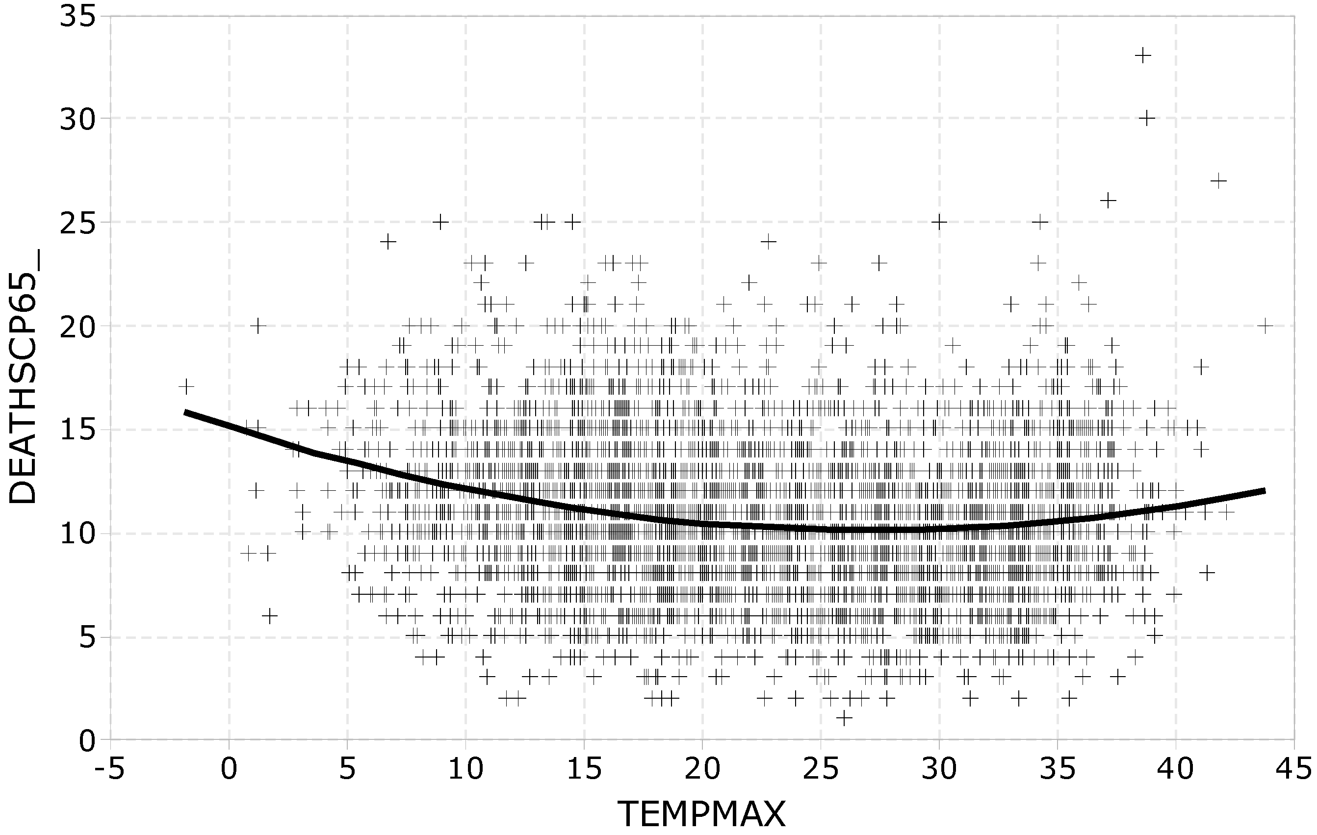
Figure 3 depicts a scatter plot of the mortality count per month as a function of the average maximum temperature values for the years 2002–2012.
Equations (1)–(4), along with the illustrative Figure 3, confirm the U-shaped functional form of such relationships that has been reported in the literature [22,30]: fatalities are lowest around maximum temperature values of 20–30 °C and increase below and above these values. It may be observed that the highest daily mortality counts are positioned in the top right corner of the graph, between 35 and 40 °C; more on this in the section presenting the cluster analysis of the sample data.
The statistical significance of the increased occurrence of cardiovascular and respiratory fatalities of people over 65 years of age, in days of temperature extremes, is examined next. As mentioned previously, the analysis considers absolute rather than apparent temperature values because their association with such deaths was more pronounced.
Table 2 compares the mean number of fatalities of people over 65 years of age, in days that were characterized by temperature extremes to the number of similar fatalities in other days. The statistical significance of the difference between fatalities, as described above, is tested by appropriate one-sided t-tests for independent samples, following an examination of the equal standard deviations assumption by Levene’s test. The first four rows in Table 2 consider days with extreme values of the minimum temperature (TEMPMIN); the next four examine days with extreme values of the maximum temperature (TEMPMAX); and the last two combine extreme temperature criteria, so that steadily cold (TEMPMIN ≤ 5 and TEMPMAX ≤ 10) and steadily hot (TEMPMIN ≥ 25 and TEMPMAX ≥ 35) days are examined.
As far as days with extreme minimum temperatures are concerned, no reliable conclusions may be drawn regarding the average number of deaths in days that had a minimum temperature above 30 degrees (TEMPMIN ≥ 30) because the total number of such days was very small (six out of a total of 4018). On days that had a minimum temperature below zero degrees (TEMPMIN ≤ 0), the average number of deaths was 12.85, which is 19.5% higher than the average number of deaths in the remaining days (10.75), with this difference being statistically significant at a 99% confidence level (t = 2.50, p = 0.006). The average number of deaths on days with a minimum temperature below 5 degrees (TEMPMIN ≤ 5) was equal to 12.53, which is 19.5% greater than the average number of deaths in the remaining days (10.65), a difference with a very high statistical significance (t = 7.73, p = 0.000). Finally, the average number of deaths on days with a minimum temperature above 25 degrees (TEMPMIN ≥ 25) is equal to 11.55, which is 8.1% greater than the average number of deaths in the remaining days (10.68), a difference that is also statistically very significant (t = 4.36, p = 0.000).
Turning our attention to the values of the maximum temperature, it is observed that fatalities were increased on days when the maximum temperature was above 35 °C (11.69 compared to 10.69 on other days), with the significance being very high in all cases (p = 0.000). On the 12 days when the maximum temperature exceeded 40 degrees, the largest increase in mean deaths was noted: 14.42 versus 10.75 on the remaining days.
The last two rows of Table 2 concern steadily cold (TEMPMIN ≤ 5 and TEMPMAX ≤ 10) or steadily hot (TEMPMIN ≥ 25 and TEMPMAX ≥ 35) days, where again there was an increase in cardiovascular and respiratory mortality of people over 65 years old, at a confidence level greater than or equal to 99.9%.

3.3. Time Series Analyses

In this section, the statistical analysis that took into consideration the temporal nature of the daily cardiovascular and respiratory mortality of people over 65 years of age (DEATHSCP65_) is presented.
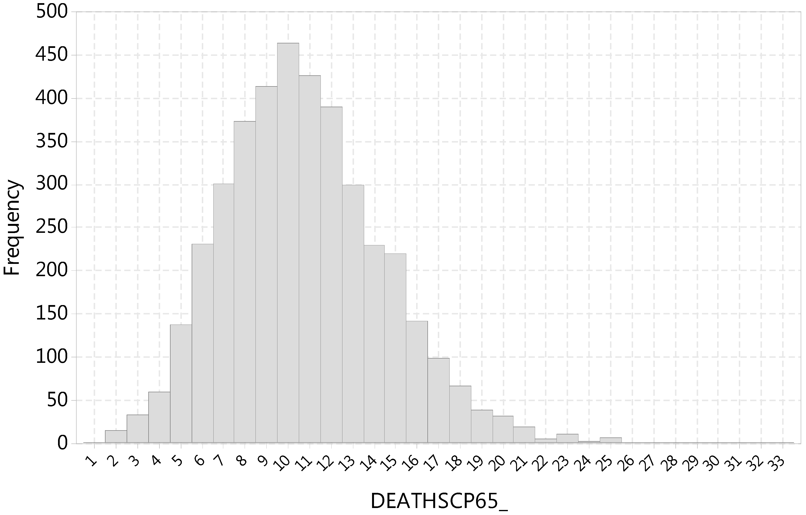
Considering the entire population of people over 65 years of age in Athens, DEATHSCP65_ is a rare event that takes positive integer values ranging from one to 33. As shown by the histogram of discrete values in Figure 4, the distribution of DEATHSCP65_ is characterized by some positive skewness. Therefore, DEATHSCP65_ should be analyzed with statistical modeling techniques appropriate for count data [40].
While count variables should be modeled based on the Poisson or negative binomial distribution [41], the histogram in Figure 4 shows that the daily mortality values are large enough for their distribution to approximate the normal distribution (although some positive skewness remains). Given that the Central Limit Theorem (CLT) states that, as the sample size increases, the sampling distribution of the mean (as in the case of regression coefficients) becomes normally distributed regardless of the shape of the original distribution of the sample [42], ordinary least Squares (OLS) could probably be used, although at some risk of being unable to detect true effects [43]. Compared to an OLS model, a distinct advantage of resorting to a Poisson or negative binomial regression would be that negative numbers would be precluded. In any case, several alternative statistical models are presented in this research.
The Poisson distribution is restricted to have the same parameter for both the mean and the variance of the count process that it models. This restriction relates to the concept of overdispersion if the Poisson distribution is used to model count processes that have a variance that is (significantly) larger than their mean (not difficult to achieve given that the variance is the square of the standard deviation). Compared to the Poisson distribution, the negative binomial distribution has separate parameters for the mean and the variance, allowing for overdispersion as well as a bigger number of zero counts [44]. In the case of DEATHSCP65_, there are no zero mortality counts; furthermore, the overall mean of the mortality daily count time series equals 10.761, with the overall variance equaling 14.039. Broken down by year, the annual mean of DEATHSCP65_ varies from 9.923 to 11.526, with the annual variance varying from 10.978 to 16.239. One of the reasons that the values of the means are approximately equal to the values of the variances is that there are no excess zero values in the daily mortality counts. It may be argued that overdispersion does not constitute a significant problem in this analysis, especially considering that the introduction of covariates (i.e., independent variables in the regression models) implies that the equality of the mean and the variance is conditional on the values of these covariates. In any case, both Poisson and negative binomial regression models were estimated in this research.
An important question in the regression of time series data is how to deal with variables that are nonstationary. A time series plot of DEATHSCP65_ (not shown) lacks any trending and wandering, but is characterized by seasonality, with most fatalities occurring in cold and hot weather. Autocorrelation function (ACF) plots (not shown) display a significant amount of positive serial correlation, with strong seasonality becoming apparent when the plots are extended into many lags. Taking the first differences of these daily mortality counts to stationarize the time series renders a series with an ACF plot (not shown) that has a highly negative AFC in the first lag and insignificant ACF values in the next lags. This is an indication of overcompensating for nonstationarity and, possibly, not in the proper way, e.g., the series could be trend stationary, in which case the proper way to stationarize it would be to subtract the trend rather than take differences. In this research, addressing nonstationarity in modeling followed the methodology of Katsouyianni et al. [45], who argued that the objective of any transformation of daily mortality counts should be to make any structures (related to trend, seasonality, and interventions) invisible in the residual plots of the fitted models, so that the final residual plots reflect only white noise.
The estimated models are shown in Table 3. The maximum likelihood method used to estimate the Poisson and negative binomial regression models requires a large sample, a stipulation satisfied in the case of this research (4017 observations with no missing data). All models were estimated with robust standard errors. The dependent variable in all models was the natural logarithm of the daily mortality counts, a transformation feasible since DEATHSCP65_ had no zero values. There was no need to estimate zero-truncated models because, although there were no zero fatalities in DEATHSCP65_, the number zero would be an acceptable value.
Resorting to cross-correlation values between mortality counts and lags of temperature or humidity to assess the delay at which the effect of these covariates on mortality is maximum [46] was not particularly helpful because these were (a) greatly influenced by seasonality and (b) unclear when the seasonality was removed, e.g., by subtracting a 30-day moving average of the mortality counts. So, lags of up to 12 days were tried, as these have been reported to represent a central value in a broad range of lags attempted in the literature [47]. Of these, only the first lag of temperature had a meaningful statistically significant coefficient and was kept in the final model formulations. The regression models presented in Table 3 do not include the square of the maximum temperature, which was included in the quadratic exposure response function presented previously [48] because its inclusion failed to render meaningful statistical coefficients for temperature and did not improve the fit.
To account for the year-to-year changes in mortality patterns (i.e., the long-term trend), two alternative formulations were tried in the models: (a) dummy variables for each year (2002–2012), or (b) a linear or a quadratic time trend [48]. Not accounting for a long-term trend at all gave models that fit the data poorly, especially after 2008. Of the two alternative formulations (dummy variables versus trend), it was decided that the yearly dummy variables would be maintained as they rendered a marginally better fit and were easier to interpret meaningfully. Seasonality was accounted for by including indicator (dummy) variables for each month (except December, to avoid perfect multicollinearity). Dummy variables were also included for each day of the week (except Sunday); alternative models including weekend dummies were also tried but were found to be inferior. The potential interaction between year and season was not accounted for because including year and month interaction terms for all 11 years of the sample would be too complex for the scheme to be useful. Finally, an attempt to account for temperature–humidity interactions [48] also failed to improve any of the models.
Regarding overdispersion, although a likelihood-ratio test showed that the negative binomial regression model was more appropriate than the Poisson one, Table 3 shows that, in fact, these two models are very similar.
Comparing the overall fit of the three models, it is observed that all information criteria (Akaike, Swartz, and Hannan–Quinn) concurred that the OLS model is superior to both the Poisson and the Negative Binomial model. Although the R-squared values are not comparable among the models (i.e., McFadden in Poisson and pseudo R-square in Negative Binomial), they show clearly that all three models fit the data very poorly. Plots of fitted vs. observed and residual values over time (not shown) showed that non-stationarity had been removed, but they also confirmed that the models fit the data poorly.
A few remarks may be made, keeping in mind the very poor fit of the models:
  • The yearly dummies that were added to account for the existence of a time trend showed that daily mortality counts appeared to decrease over time, especially after 2008 (with the corresponding negative coefficients being statistically significant, at a 5% or 10% level, in the Poisson and the negative binomial models).
  • Regarding the day of the week, it should be kept in mind that the day of the week coefficients compared the effect of the corresponding day of the week to Sunday, which was the day for which no dummy was included in the models. Mondays appeared to have a statistically significant aggravating effect on mortality in all models, with no other days of the week being associated with increased or decreased mortality in a statistically significant way.
  • The monthly dummy variables compared the effect of the months to December, which was the month for which no dummy was included in the models. Thus, it was shown that the cold months aggravated mortality while the summer months alleviated it (more on the effect of temperature later), with January being the worst and September being the best months, mortality-wise.
  • While the maximum temperature (of the day the fatality occurred) did not appear to have a significant effect on mortality, the maximum temperature lagged by one day had a significant aggravating effect on mortality, in all models. This shows that it takes one day for the temperature to have a drastic effect on the cardiovascular and respiratory health of people over 65 years of age, a fact that sheds more light on the literature findings cited previously [47]. Unfortunately, the very poor fit of all the models adds ambiguity to this finding. The number of heatwave days also had a clear, statistically significant effect on mortality, showing that, as a heatwave is prolonged, it is associated with increased mortality.
  • Turning to humidity, one sees that the maximum humidity has a negative effect on mortality that is statistically significant (at an 18% confidence level or less). Apparently, there are low-humidity days that are characterized by high cardiovascular and respiratory health issues of people over 65 years of age. More on this association will be presented in the cluster analysis results, presented in the next section.
It is worth mentioning that air pollutant (ozone, sulfur dioxide, and nitrogen dioxide) concentrations were employed as independent variables but were found to have statistically insignificant coefficients and were, thus, excluded from the models; particulate concentrations, which (as mentioned previously) were available only for a few years towards the end of the study period, were characterized by great gaps of missing data, and thus were of no use in time series analysis.
To recap the findings of the time series models, mortality appeared to fall after 2008, a result possibly pointing to a better level of preparedness of the state and society in Greece. In addition, it was found that the effect of temperature was most significant at a lag of one day. Nevertheless, it was concluded that a time series approach had mediocre success in discovering associations in the mortality counts of Athens and it was decided that an alternative multivariate analysis approach would be attempted in the next section. To the knowledge of the authors, such an approach has not been tried before in temperature–mortality research.

3.4. Cluster Analysis

Following the estimation of time series models of the cardiovascular and respiratory mortality of people over 65 years of age, an attempt is made now to discover meaningful associations between mortality, temperature, and humidity by carrying out a cluster analysis. It was decided to limit the analysis on the months of May to September to analyze the effect of high temperatures. The usage of cluster analysis constitutes a rather novel approach in the mortality–temperature literature.
Estimates regarding the number of clusters, based in part on the multimodal shape of the distribution of temperatures, had indicated the presence of three or more (some possible small) clusters [49]. On the issue of sample size, Formann [50], as cited by Mooi and Sarstedt [51] (p. 243), recommends a sample of at least 2m cases, where m equals the number of clustering variables. These recommendations imply that a sample size of 1678 observations with no missing data (which was left for clustering, as shown in Table 4) could support up to 10 variables (210 = 1024 while 211 = 2048).
To arrive at a relatively robust clustering scheme, Ward’s method, with the squared Euclidean distance being the recommended distance metric [52], was run to estimate and compare three-, four-, five-, and six-cluster solutions that were suggested by the dendrogram (not shown). Of these, the five- and six-cluster solutions were particularly appealing because they classified heatwave days into their own cluster. A two-step cluster analysis (effective with large datasets [51]), which was run (with SPSS) to determine the final number of clusters and membership scheme, rendered the six-cluster solution optimal. This was chosen as the final clustering scheme and is tabulated in Table 4, which shows the centroid values of variables used in the cluster analysis. To facilitate interpretation, the clusters were numbered in order of increasing mortality.
Table 5 shows the centroid or percentage values of the variables that were not used in the cluster analysis.
To confirm the significance of the selected clustering scheme, it is not enough to consider the high significance of ANOVA or Welch tests, shown in Table 4 and Table 5: this was expected because of the large sample size. Therefore, a multiple discriminant analysis was run on the clustering variables of Table 5, which employed five canonical discriminant functions (with eigenvalues of 4.756, 1.657, 1.172, 0.359, and 0.038) and cumulatively accounted for 100% of the variance. Prior probabilities were not adjusted for group size, so as not to bias the classification results with a priori knowledge of cluster sizes. The classification results (confusion matrix) of the multiple discriminant analysis are (is) shown in Table 6.
The membership in Clusters 1 to 6 was classified correctly in 89.2, 96.1, 92.4, 97.4, 64.7, and 97.8% of the cases. Of these, the membership in Cluster 5 (the heatwave cluster, as explained below) was classified correctly in 64.7% of the cases, with the rest 31.4% misclassified into Cluster 6 (the cluster with the highest mortality counts, a cluster similar to Cluster 5 yet distinct in an important way, as will be discussed below) and 3.9% into Cluster 2. The overall clustering scheme is deemed satisfactory since 93.8% of the total cases were classified into the correct cluster.
Having validated the clustering scheme, attention now turns to the description of the six clusters.
  • Cluster 1 had the lowest mortality, 7.77 daily fatalities of people over 65 due to cardiovascular and respiratory causes. The minimum and maximum temperature centroids were equal to 23.64 and 32.94 °C respectively, with their apparent values equal to 26.35 and 34.01 °C, respectively, certainly not the lowest among the clusters. The minimum and maximum relative humidity were equal to 29.42% and 60.9%, respectively, among the lowest in the clusters. The cases of this cluster were dispersed in August, July, and June, mostly, with fewer cases being in September and fewest in May.
  • Cluster 2 was also a cluster of low mortality, with 8.15 daily fatalities. Centroid minimum and maximum temperatures equaled 18.54 and 26.07 °C, respectively (or 22.99–30.28 °C in apparent values), among the lowest in the clusters. The minimum and maximum relative humidity were equal to 53.09% and 85.32%, respectively, the highest among all the clusters. Almost half of the cases of this cluster were in September, with about one-third in May, almost one-fifth in June, and very few in July and August.
  • The mortality centroid jumped to 10.66 in Cluster 3, which had minimum and maximum temperatures equal to 17.82 and 26.68 °C, respectively (with 19.99 and 27.99 °C being the apparent values). The minimum and maximum relative humidity were equal to 36.83% and 71.75%, respectively. Over half of the cases of this cluster were in May, with about one-fifth in September and June; July and August contained very few cases belonging to this cluster.
  • Cluster 4 had a centroid daily mortality equal to 11.02, and minimum and maximum centroid temperatures equal to 23.72 and 32.88 °C respectively (and apparent values equal to 29.24 and 37.9 °C). The minimum and maximum relative humidity were high, equal to 44.81% and 77.46%, respectively. This cluster contained cases mostly from August and July, with fewer from September and June, and very few from May.
  • Cluster 5 was the heatwave cluster, with a centroid value of 2.745 heatwave days. Its mortality at the centroid was equal to 12.98, which was the second highest among all six clusters. The heatwave cluster had the second highest minimum and maximum centroid temperatures, equal to 28.25 to 38.57 °C, respectively (apparent values equal to 30.86 and 39.49 °C). The minimum and maximum relative humidity were the smallest among the six clusters, equal to 25.14% and 52.37% respectively. Over 90% of the cases in this cluster fell in the months of July and August, with a few cases in June and almost none in May and September.
  • Finally, Cluster 6 had the highest centroid mortality (13.24), yet it was characterized by the second highest centroid minimum and maximum temperatures, equal to 25.35 and 34.82 °C, respectively (with 27.73 and 35.44 °C being their apparent values), which was rather surprising. Like Cluster 5, Cluster 6 was also characterized by low values of the minimum and maximum relative humidity (26.29% and 54.05%, respectively). Finally, Cluster 6 contained cases from July, August and July, with fewer cases from September and May.
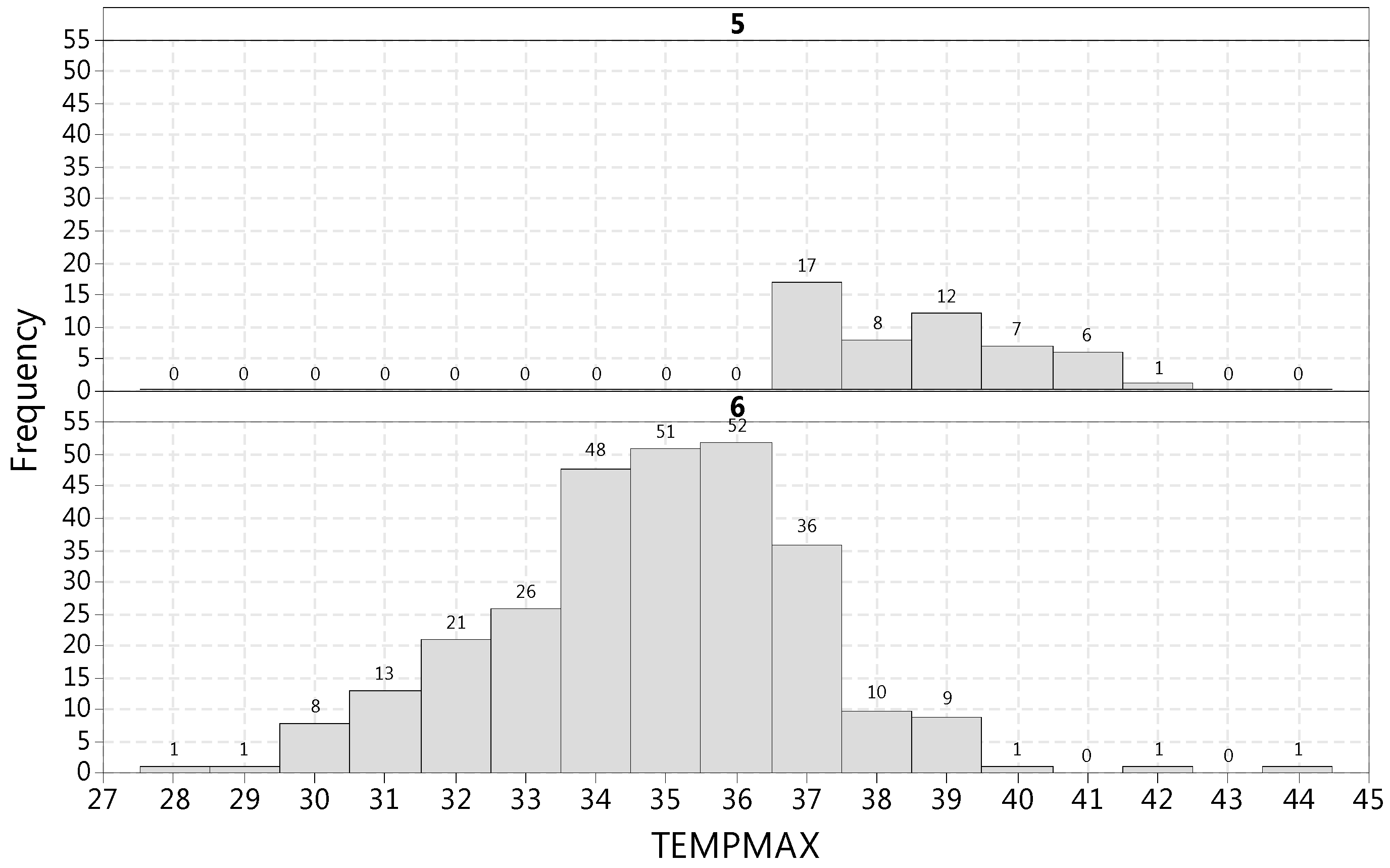
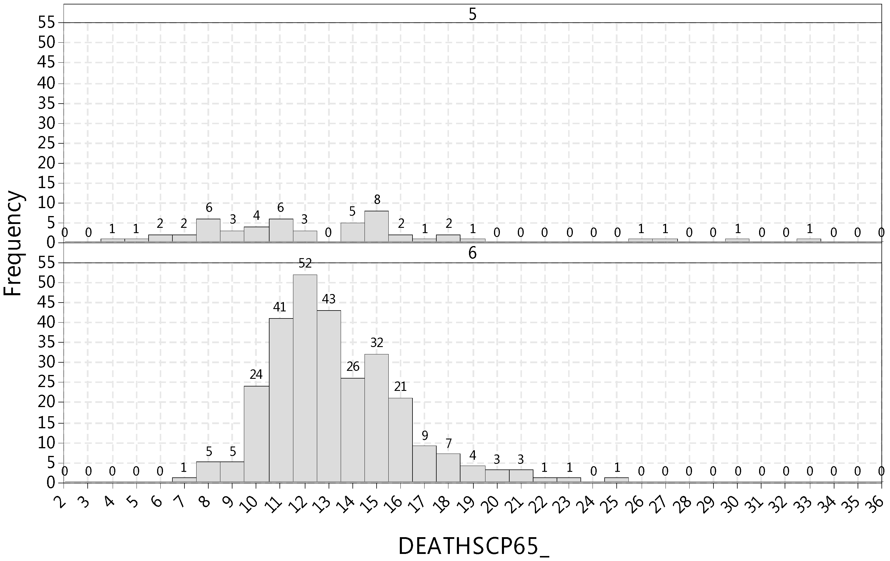
The apparent discrepancy between temperature and mortality of clusters 5 and 6 was investigated further with the aid of the histograms displayed in Figure 5 and Figure 6. Cluster 5 contained cases with the maximum temperature ranging from 36.5 to 41.8 °C (top panel of Figure 5) and the mortality varying from four to 33 daily fatalities (top panel of Figure 6). Cluster 6 contained cases with the maximum temperature ranging from 28.4 to 43.8 °C (bottom panel of Figure 5), with the mortality varying from seven to 25 daily fatalities (bottom panel of Figure 6). Yet, as shown in Figure 6, the mortality of Cluster 5 was essentially distributed from 4 to 19, with four distant observations raising the maximum value to 33. While Cluster 6 contained a few unusually hot days (that were not part of a heatwave), the highest maximum temperature day (43.8 °C) being one of them (bottom panel of Figure 5), it was not these very few outlying observations that caused the higher centroid mortality of Cluster 6, but mostly the fact that the entire distribution of mortality of Cluster 6 was shifted to the right (i.e., towards higher fatality values) compared to Cluster 5 (Figure 6).
Neither the weekend nor the weekday indicator variables contributed in a significant or meaningful way to discerning any differences among the clusters. Finally, air pollutant concentrations were not found to contribute meaningfully in any clustering scheme, while particulate concentrations (being available for a few years only and with many missing values) were excluded from the analysis because they would greatly reduce the sample size.
The approach of cluster analysis overcame the problem of analyzing discontinuous observations, i.e., May to September only. The findings shed light on the interaction of temperature and mortality. The mortality of Cluster 5 (the heatwave cluster) is important because heatwaves exacerbate the UHI [10], yet the existence of Cluster 6 showed that older people perhaps get acclimated and develop better responses to conditions prevalent in heatwaves, thus running a smaller risk of suffering adverse health effects compared to isolated days of very high temperature.

4. Discussion

Published research that examines the effects of high temperatures on human health includes (a) studies that examine a single city such as Ahmedabad [19], Athens [37], Madrid [53], Budapest [54], Dublin [55], Montreal [56], Toronto [57], Sydney [58], Brisbane [59], and São Paulo [60]; (b) studies that examine a relatively small geographical region such as the state of Arizona [28] or the Netherlands [61]; and (c) multiple city studies such as [22,24]. Compared to the state of the art, this research is a single-city analysis that reflects significant potential, given (a) the size of the city, (b) its lasting exposure to high temperatures, and (c) the occurrence of heat waves and the increasing share of elderly people in the city’s population. Furthermore, the results of this research reflect the period until 2012 (thus they are considerably updated as compared to previous studies in this region, with 2004 being the end year), facilitating new analyses of the cardiovascular and respiratory mortality of people over 65 years of age. To this end, this paper may be used as a reference for studies in other cities in southern Europe.
As mentioned before, the average daily cardiovascular and respiratory mortality count of people over 65 years of age for the entire sampling period (2002 to 2012) was equal to 10.76 (with a minimum of one and a maximum of 33). Compared to this value, the excess mortality count for Cluster 6 was +23%, while for Cluster 5 (the heatwave cluster) it was +20.6%. For comparison purposes, the excess mortality counts for the other four clusters were: +2.42% for Cluster 4, −0.929% for Cluster 3, −24.3% for Cluster 2, and −27.8% for Cluster 1. So, Clusters 6 and 5 were clusters of significantly increased and Clusters 2 and 1 were clusters of significantly decreased daily cardiovascular and respiratory mortality count of people over 65 years of age (13.24 and 12.98 versus 8.15 and 7.77 daily deaths correspondingly, a reduction of approximately 38%).
The minimum apparent temperature of 30.86 °C for cluster 5 (heatwave) was near the value of 32.7 °C found by Baccini et al. [22] to constitute the threshold of increased susceptibility for Athens, and the value of 33 °C that was found to increase the mortality risk six-fold [30]; on the other hand, the minimum apparent temperature of Cluster 6, 27.73 °C, was quite a bit lower. In other words, (a) very hot days outside heatwave periods and (b) heatwave spells represented the worst periods in terms of excess cardiovascular and respiratory mortality in people over 65 years of age.
Per the findings of this research study, and taking into consideration that (a) the combined effect of very hot days or heatwaves and the urban heat island translate into excessive cardiovascular and respiratory mortality (for people over 65 years of age), and (b) the share of people above 65 years of age is increasing in cities in developed countries due to aging, the improvement of the thermal environment in urban areas is considered to be of great priority. Significant attention needs to be given to efforts towards the reduction of mortality during heatwaves and very hot days, along with efforts towards the amelioration of fuel poverty and impacts on low-income families due to heat stress [62,63,64].
What will the future look like in terms of heat-related mortality, and what can we do about it? There is little doubt that the increased frequency of hot days and warm spells will exacerbate the UHI effects [10], causing health problems [65]. Zuo et al. [66] provide a comprehensive review of the impacts of heat waves and corresponding measures. According to this review, a heat wave will often involve a combination of environmental factors (such as temperature, humidity, radiation, and wind speed) and social or cultural factors. In terms of the impact of heat waves, the review shows that, in the majority of the related studies, more focus is given to environmental issues such as water quality, power consumption, peak demand, and pollution and health issues. Cost and social issues derived from heat waves are comparatively overlooked.
Stone et al. [67] developed a set of climate projections for three urban areas in the USA (Atlanta, Georgia; Philadelphia, Pennsylvania; and Phoenix, Arizona), establishing that temperature reductions could be achieved through a combination of changes in vegetation cover and surface albedo, and found heat management strategies to be effective in offsetting excess mortality during both heatwave and non-heatwave conditions. Such interventions may also be considered for Athens and other urban areas in the Mediterranean.
Heaviside et al. (2016) found that the UHI provided almost 50% of the total heat-related mortality during the 2003 heatwave in the West Midlands [68]. The results of this research also underline the importance of alleviating the UHI effect. Since the UHI effect in Athens has been reported to have a mean daily intensity ranging from about 5 °C to over 10 °C for the major central area [69,70,71,72,73], Table 4 shows that a modest reduction in temperatures, such as by usage of reflective coating [74], would bring environmental conditions from those of Clusters 6 or 5 (heatwave) to those of Clusters 2 or 1, reducing mortality from about 13 to about 8 (38%), an extremely significant public health achievement.
Considerations for extending this research include: investigating the association of socioeconomic variables such as income [19] and isolation [24] with mortality [27]; accounting for harvesting [24]; estimating disaggregate models identifying and marking the appearance and duration of heatwaves, as discussed by Nastos and Matzarakis [30]; and assessing the effect of vegetative and albedo interventions on heat-related mortality [66].

Acknowledgments

The authors thank the Hellenic Statistical Authority (http://www.statistics.gr/en/home) and the Directorate for Air Pollution and Noise Control of the Ministry of the Environment and Climate Change (http://www.ypeka.gr/Default.aspx?tabid=3 7&locale=en-US&language=el-GR) for providing the data used in this research, as well as Terry Nadasdi and Stefan Sinclair for their online Spell Check Plus (http://spellcheckplus.com), which was used for proofing the entire manuscript.

Author Contributions

John Paravantis contributed to the literature review, carried out the data analysis, and wrote the paper; Mat Santamouris conceived the research, and contributed to the literature review, the statistical analysis and discussion; Constantinos Cartalis contributed to the literature review, the statistical analysis and the discussion; Chrysanthi Efthymiou contributed to the literature review and the discussion; Nikoletta Kontoulis wrote the literature review and contributed to the discussion.

Conflicts of Interest

The authors declare no conflict of interest.

Abbreviations

The following abbreviations are used in this manuscript, including variable names (with variable units in parentheses):
APPTEMPMAXdaily maximum apparent temperature (°C)
APPTEMPMINdaily minimum apparent temperature (°C)
DEATHSCPtotal daily fatalities attributed to cardiovascular or respiratory causes
DEATHSCP_65daily fatalities below 65 years of age, attributed to cardiovascular or respiratory causes
DEATHSCP65_daily fatalities above 65 years of age, attributed to cardiovascular or respiratory causes
HEATWAVEDAYSnumber of consecutive days in heatwave
MDPIMultidisciplinary Digital Publishing Institute
RELHUMAXmaximum daily relative humidity (%)
RELHUMINminimum daily relative humidity (%)
TEMPMAXmaximum daily temperature (°C)
TEMPMINminimum daily temperature (°C)
UHIUrban Heat Island
WEEKENDdummy variable (1 = Saturday or Sunday, 2 = other days of the week)

References

  1. Mitchell, D.; Heaviside, C.; Vardoulakis, S.; Huntingford, C.; Masato, G.; Guillod, B.P.; Frumhoff, P.; Bowery, A.; Wallom, D.; Allen, M. Attributing human mortality during extreme heatwaves to anthropogenic climate change. Environ. Res. Lett. 2016, 11, 7. [Google Scholar] [CrossRef]
  2. Santamouris, M.; Kolokotsa, D. (Eds.) Urban Climate Mitigation Techniques; Routledge: London, UK, 2016. [Google Scholar]
  3. Meier, A. Countermeasures to Urban Heat Islands: A Global View; Ernest Orlando Lawrence Berkeley National Laboratory: Berkeley, CA, USA, 2006. [Google Scholar]
  4. Santamouris, M. Analyzing the heat island magnitude and characteristics in one hundred Asian and Australian cities and regions. Sci. Total Environ. 2015, 512, 582–598. [Google Scholar] [CrossRef] [PubMed]
  5. Santamouris, M. Innovating to zero the building sector in Europe: Minimising the energy consumption, eradication of the energy poverty and mitigating the local climate change. Sol. Energy 2016, 128, 61–94. [Google Scholar] [CrossRef]
  6. Santamouris, M. On the energy impact of urban heat island and global warming on buildings. Energy Build. 2014, 82, 100–113. [Google Scholar] [CrossRef]
  7. Santamouris, M.; Cartalis, C.; Synnefa, A.; Kolokotsa, D. On the impact of urban heat island and global warming on the power demand and electricity consumption of buildings—A review. Energy Build. 2015, 98, 119–124. [Google Scholar] [CrossRef]
  8. Pantavou, K.; Theoharatos, G.; Mavrakis, A.; Santamouris, M. Evaluating thermal comfort conditions and health responses during an extremely hot summer in Athens. Build. Environ. 2011, 46, 339–344. [Google Scholar] [CrossRef]
  9. Sakka, A.; Santamouris, M.; Livada, I.; Nicol, F.; Wilson, M. On the thermal performance of low income housing during heatwaves. Energy Build. 2012, 49, 69–77. [Google Scholar] [CrossRef]
  10. Li, D.; Bou-Zeid, E. Synergistic interactions between urban heat islands and heatwaves: The impact in cities is larger than the sum of its parts. J. Appl. Meteorol. 2013, 52, 2051–2064. [Google Scholar] [CrossRef]
  11. Li, D.; Sun, T.; Liu, M.; Yang, L.; Wang, L.; Gao, Z. Contrasting responses of urban and rural surface energy budgets to heatwaves explain synergies between urban heat islands and heatwaves. Environ. Res. Lett. 2015, 10, 5. [Google Scholar] [CrossRef]
  12. Stathopoulou, E.; Mihalakakou, G.; Santamouris, M.; Bagiorgas, H.S. On the impact of temperature on tropospheric ozone concentration levels in urban environments. J. Earth Syst. Sci. 2008, 117, 227–236. [Google Scholar] [CrossRef]
  13. Changnon, S.A.; Kunkel, K.E.; Reinke, B.C. Impact and responses to the 1995 heatwave: A call to action. Bull. Am. Meteorol. Soc. 1996, 77, 1497–1506. [Google Scholar] [CrossRef]
  14. Santamouris, M.; Kolokotsa, D. On the impact of urban overheating and extreme climatic conditions on housing energy comfort and environmental quality of vulnerable population in Europe. Energy Build. 2015, 98, 125–133. [Google Scholar] [CrossRef]
  15. Voogt, J. Urban Heat Island. Encyclopedia of Global Environmental Change; John Wiley & Sons, Ltd.: Chichester, UK, 2002. [Google Scholar]
  16. Robine, J.-M.; Cheung, S.L.K.; Le Roy, S.; Van Oyen, H.; Griffiths, C.; Michel, J.-P.; Herrmann, F.R. Death toll exceeded 70,000 in Europe during the summer of 2003. C. R. Biol. 2008, 331, 171–178. [Google Scholar] [CrossRef] [PubMed]
  17. Anderson, B.G.; Bell, M.L. Weather-related mortality: How heat, cold, and heatwaves affect mortality in the United States. Epidemiology 2009, 20, 205–213. [Google Scholar] [CrossRef] [PubMed]
  18. Basu, R. High ambient temperature and mortality: A review of epidemiologic studies from 2001 to 2008. Environ. Health 2009, 8, 40. [Google Scholar] [CrossRef] [PubMed]
  19. Azhar, G.S.; Mavalankar, D.; Nori-Sarma, A.; Rajiva, A.; Dutta, P.; Jaiswal, A.; Sheffield, P.; Knowlton, K.; Hess, J.J. Heat-related mortality in India: Excess all-cause mortality associated with the 2010 Ahmedabad Heatwave. PLoS ONE 2014, 9, e91831. [Google Scholar] [CrossRef] [PubMed]
  20. Pan, W.H.; Li, L.A.; Tsai, M.J. Temperature extremes and mortality from coronary heart disease and cerebral infarction in elderly Chinese. Lancet 1995, 345, 353–355. [Google Scholar] [CrossRef]
  21. Santamouris, M. Local climate change: Assessing the impact and mitigating the heat. In Energia, Ambiente e Innovazione; Number 2; Padovani, L.M., Puglisi, G., Eds.; ENEA: Rome, Italy, 2016; pp. 98–103. [Google Scholar]
  22. Baccini, M.; Biggeri, A.; Accetta, G.; Kosatsky, T.; Katsouyanni, K.; Analitis, A.; Ross Anderson, H.; Bisanti, L.; D’Ippoliti, D.; Danova, J.; et al. Heat effects on mortality in 15 European cities. Epidemiology 2008, 19, 711–719. [Google Scholar] [CrossRef] [PubMed]
  23. Hajat, S.; Armstrong, B.; Baccini, M.; Biggeri, A.; Bisanti, L.; Russo, A.; Paldy, A.; Menne, B.; Kosatsky, T. Impact of high temperatures on mortality: Is there an added heatwave effect? Epidemiology 2006, 17, 632–638. [Google Scholar] [CrossRef] [PubMed]
  24. D’Ippoliti, D.; Michelozzi, P.; Marino, C.; de’ Donato, F.; Menne, B.; Katsouyanni, K.; Kirchmayer, U.; Analitis, A.; Medina-Ramón, M.; Paldy, A.; et al. The impact of heatwaves on mortality in 9 European cities: Results from the EuroHEAT project. Environ. Health 2010, 9, 37. [Google Scholar] [CrossRef] [PubMed]
  25. Díaz, J.; Garcia, R.; de Velazquez, C.F.; Hernandez, E.; Lopez, C.; Otero, A. Effects of extremely hot days on people older than 65 years in Seville (Spain) from 1986 to 1997. Int. J. Biometeorol. 2002, 46, 145–149. [Google Scholar] [PubMed]
  26. National Research Council. Reconciling Observations of Global Temperature Change; National Research Council: Washington, DC, USA, 2000. [Google Scholar]
  27. Basu, R.; Dominici, F.; Samet, J.M. Temperature and mortality among the elderly in the United States—A comparison of epidemiologic methods. Epidemiology 2005, 16, 58–66. [Google Scholar] [CrossRef] [PubMed]
  28. Harlan, S.L.; Chowell, G.; Yang, S.; Petitti, D.B.; Morales Butler, E.J.; Ruddell, B.L.; Ruddell, D.M. Heat-related deaths in hot cities: Estimates of human tolerance to high temperature thresholds. Int. J. Environ. Res. Public Health 2014, 11, 3304–3326. [Google Scholar] [CrossRef] [PubMed]
  29. National Oceanic and Atmospheric Administration’s National Weather Service Glossary. Available online: http://w1.weather.gov/glossary (accessed on 25 January 2016).
  30. Nastos, P.T.; Matzarakis, A. The effect of air temperature and human thermal indices on mortality in Athens, Greece. Theor. Appl. Climatol. 2011, 108, 591–599. [Google Scholar] [CrossRef]
  31. Dilaveris, P.; Synetos, A.; Giannopoulos, G.; Gialafos, E.; Pantazis, A.; Stefanadis, C. Climate impacts on myocardial infarction deaths in the Athens Territory: The CLIMATE study. Heart 2006, 92, 1747–1751. [Google Scholar] [CrossRef] [PubMed]
  32. Schär, C.; Vidale, P.; Luthi, D.; Frei, C.; Haberi, C.; Liniger, M.; Appenzeller, C. The role of increasing temperature variability in European summer heatwaves. Nature 2004, 427, 332–336. [Google Scholar] [CrossRef] [PubMed]
  33. Meehl, G.A.; Tebaldi, C. More intense, more frequent, and longer lasting heatwaves in the 21st century. Science 2004, 305, 994–997. [Google Scholar] [CrossRef] [PubMed]
  34. Clark, R.T.; Brown, S.J.; Murphy, J.M. Modeling Northern Hemisphere summer heat extreme changes and their uncertainties using a physics ensemble of climate sensitivity experiments. J. Clim. 2006, 19, 4418–4435. [Google Scholar] [CrossRef]
  35. Fischer, M.; Schär, C. Consistent geographical patterns of changes in high-impact European heatwaves. Nat. Geosci. 2010, 3, 398–403. [Google Scholar] [CrossRef]
  36. Papanastasiou, D.; Melas, D.; Kambezidis, H. Heatwaves characteristics and their relation to air quality in Athens. Glob. NEST J. 2014, 16, 919–928. [Google Scholar]
  37. Theoharatos, G.; Pantavou, K.; Mavrakis, A.; Spanou, A.; Katavoutas, G.; Efstathiou, P.; Mpekas, P.; Asimakopoulos, D. Heatwaves observed in 2007 in Athens, Greece: Synoptic conditions, bioclimatological assessment, air quality levels and health effects. Environ. Res. 2010, 110, 152–161. [Google Scholar] [CrossRef] [PubMed]
  38. Giannopoulos, P. Extreme Summer Temperatures in Greece Heatwaves. Hellenic National Meteorological Service. Available online: http://meteo.hr/SEECOF08/day2/2-18.pdf (accessed on 6 August 2016).
  39. Baiocchi, G.; Distaso, W. GRETL: Econometric software for the GNU generation. J. Appl. Econ. 2003, 18, 105–110. [Google Scholar] [CrossRef]
  40. Winkelmann, R. Counting on count data models: Quantitative policy evaluation can benefit from a rich set of econometric methods for analyzing count data. IZA World Labor 2015. [Google Scholar] [CrossRef]
  41. Fokianos, K. Statistical analysis of count time series models: A GLM perspective. In Handbook of Discrete-Valued Time Series; Davis, R., Holan, S., Lund, R., Ravishanker, N., Eds.; Chapman & Hall: London, UK, 2016; pp. 3–28. [Google Scholar]
  42. Cohen, J.; Cohen, P.; West, S.G.; Aiken, L.S. Applied Multiple Regression/Correlation Analysis for the Behavioral Sciences; Lawrence Erlbaum Associates: Mahwah, NJ, USA, 2003. [Google Scholar]
  43. Wilcox, R.R. Introduction to Robust Estimation and Hypothesis Testing, 2nd ed.; Elsevier Academic Press: New York, NY, USA, 2005. [Google Scholar]
  44. Karlis, D.; Hermans, E. Time Series Models for Road Safety Accident Prediction. Report Number RA-MOW-2011-020. Available online: http://imob.ifolks.be/sites/default/files/RA-MOW-2011-020.pdf (accessed on 12 April 2017).
  45. Katsouyanni, K.; Schwartz, J.; Spix, C.; Touloumi, G.; Zmirou, D.; Zanobetti, A.; Wojtyniak, B.; Vonk, J.M.; Tobias, A.; Pönkä, A.; et al. Short term effects of air pollution on health: A European approach using epidemiologic time series data: The APHEA protocol. J. Epidemiol. Community Health 1996, 50 (Suppl. 1), S12–S18. [Google Scholar] [CrossRef] [PubMed]
  46. Gouveia, N.; Fletcher, T. Time series analysis of air pollution and mortality: Effects by cause, age and socioeconomic status. J. Epidemiol. Community Health 2000, 54, 750–755. [Google Scholar] [CrossRef] [PubMed]
  47. Gosling, S.N.; McGregor, G.R.; Páldy, A. Climate change and heat-related mortality in six cities. Part 1: Model construction and validation. Int. J. Biometeorol. 2007, 51, 525–540. [Google Scholar] [CrossRef] [PubMed]
  48. Schwartz, J.; Spix, C.; Touloumi, G.; Bachárová, L.; Barumamdzadeh, T.; le Tertre, A.; Piekarksi, T.; de Leon, A.P.; Pönkä, A.; Rossi, G.; et al. Methodological issues in studies of air pollution and daily counts of deaths or hospital admissions. J. Epidemiol. Community Health 1996, 50 (Suppl. 1), S3–S11. [Google Scholar] [CrossRef] [PubMed]
  49. Everitt, B.S.; Landau, S.; Leese, M.; Stahl, D. Cluster Analysis, 5th ed.; Wiley and Sons: West Sussex, UK, 2011. [Google Scholar]
  50. Formann, A.K. Die Latent-Class-Analyse: Einführung in Die Theorie und Anwendung; Beltz: Weinheim, Germany, 1984. [Google Scholar]
  51. Mooi, E.; Sarstedt, M. A Concise Guide to Market Research: The Process, Data, and Methods Using IBM SPSS Statistics; Springer: Berlin/Heidelberg, Germany, 2011. [Google Scholar]
  52. Romesburg, C.H. Cluster Analysis for Researchers; Lulu Press: Morrisville, NC, USA, 2004. [Google Scholar]
  53. Díaz, J.; Linares, C.; Tobías, A. Impact of extreme temperatures on daily mortality in Madrid (Spain) among the 45–64 age-group. Int. J. Biometeorol. 2006, 50, 342–348. [Google Scholar] [CrossRef] [PubMed]
  54. Bobvos, J.; Fazekas, B.; Pàldy, A. Assessment of heat-related mortality in Budapest from 2000 to 2010 by different indicators. Q. J. Hung. Meteorol. Serv. 2015, 119, 143–158. [Google Scholar]
  55. Goodman, P.G.; Dockery, D.W.; Clancy, L. Cause-specific mortality and the extended effects of particulate pollution and temperature exposure. Environ. Health Perspect. 2004, 112, 179–185. [Google Scholar] [CrossRef] [PubMed]
  56. Kolb, S.; Radon, K.; Valois, M.F.; Héguy, L.; Goldberg, M.S. The short-term influence of weather on daily mortality in congestive heart failure. Arch. Environ. Occup. Health 2007, 62, 169–176. [Google Scholar] [CrossRef] [PubMed]
  57. Rainham, D.G.; Smoyer-Tomic, K.E. The role of air pollution in the relationship between a heat stress index and human mortality in Toronto. Environ. Res. 2003, 93, 9–19. [Google Scholar] [CrossRef]
  58. Vaneckova, P.; Hart, M.A.; Beggs, P.J.; de Dear, R.J. Synoptic analysis of heat-related mortality in Sydney, Australia, 1993–2001. Int. J. Biometeorol. 2008, 52, 439–451. [Google Scholar] [CrossRef] [PubMed]
  59. Ren, C.; Williams, G.M.; Tong, S. Does particulate matter modify the association between temperature and cardiorespiratory diseases? Environ. Health Perspect. 2006, 114, 1690–1696. [Google Scholar] [CrossRef] [PubMed]
  60. Gouveia, N.; Hajat, S. Armstrong, B. Socioeconomic differentials in the temperature-mortality relationship in São Paulo, Brazil. Int. J. Epidemiol. 2003, 32, 390–397. [Google Scholar] [CrossRef] [PubMed]
  61. Huynen, M.M.T.E.; Martens, P.; Schram, D.; Weijenberg, M.P.; Kunst, A.E. The impact of heat waves and cold spells on mortality rates in the Dutch population. Environ. Health Perspect. 2001, 109, 463–470. [Google Scholar] [CrossRef] [PubMed]
  62. Santamouris, M.; Paravantis, J.A.; Founda, D.; Kolokotsa, D.; Michalakakou, P.; Papadopoulos, A.M.; Kontoulis, N.; Tzavali, A.; Stigka, E.K.; Ioannidis, Z.; et al. Financial crisis and energy consumption: A household survey in Greece. Energy Build. 2013, 65, 477–487. [Google Scholar] [CrossRef]
  63. Santamouris, M.; Alevizos, S.M.; Aslanoglou, L.; Mantzios, D.; Milonas, P.; Sarelli, I.; Karatasou, S.; Cartalis, K.; Paravantis, J.A. Freezing the poor-indoor environmental quality in low and very low income households during the winter period in Athens. Energy Build. 2014, 70, 61–70. [Google Scholar] [CrossRef]
  64. Paravantis, J.A.; Santamouris, M. An analysis of indoor temperature measurements in low and very low income housing in Athens, Greece. Adv. Build. Energy Res. 2016, 10, 20–45. [Google Scholar] [CrossRef]
  65. Sillman, S.; Samson, P.J. The impact of temperature on oxidant formation in urban, polluted rural and remote environments. J. Geophys. Res. 1995, 100, 11497–11508. [Google Scholar] [CrossRef]
  66. Zuo, J.; Pullen, S.; Palmer, J.; Bennetts, H.; Chileshe, N.; Ma, T. Impacts of heat waves and corresponding measures: A review. J. Clean. Prod. 2015, 92, 1–12. [Google Scholar] [CrossRef]
  67. Stone, B.; Vargo, J.; Liu, P.; Habeeb, D.; Delucia, A.; Trail, M.; Hu, Y.; Russell, A. Avoided Heat-Related Mortality through Climate Adaptation Strategies in Three US Cities. PLoS ONE 2014, 9, e100852. [Google Scholar] [CrossRef] [PubMed]
  68. Heaviside, C.; Vardoulakis, S.; Cai, X.M. Attribution of mortality to the urban heat island during heatwaves in the West Midlands, UK. Environ Health 2016. [Google Scholar] [CrossRef] [PubMed]
  69. Santamouris, M.; Mihalakakou, G.; Papanikolaou, N.; Assimakopoulos, D.N. A neural network approach for modelling the heat island phenomenon in urban areas during the summer period. Geophys. Res. Lett. 1999, 26, 337–340. [Google Scholar] [CrossRef]
  70. Livada, I.; Santamouris, M.; Niachou, K.; Papanikolaou, N.; Mihalakakou, G. Determination of places in the great Athens area where the heat island effect is observed. Theor. Appl. Climatol. 2002, 71, 219–230. [Google Scholar] [CrossRef]
  71. Mihalakakou, G.; Flocas, H.; Santamouris, M.; Helmis, C. The impact of synoptic scale atmospheric circulation on the urban heat island effect over Athens, Greece. J. Appl. Meteorol. 2002, 41, 519–527. [Google Scholar]
  72. Stathopoulou, M.; Cartalis, C. Daytime urban heat islands from Landsat ETM+ and Corine land cover data: An application to major cities in Greece. Sol. Energy 2006, 81, 358–368. [Google Scholar] [CrossRef]
  73. Giannopoulou, K.; Livada, I.; Santamouris, M.; Saliari, M.; Assimakopoulos, M.; Caouris, Y.G. On the characteristics of the summer urban heat island in Athens, Greece. Sustain. Cities Soc. 2011, 1, 16–28. [Google Scholar] [CrossRef]
  74. Synnefa, A.; Santamouris, M.; Livada, I. A study of the thermal performance of reflective coatings for the urban environment. Sol. Energy 2006, 80, 968–981. [Google Scholar] [CrossRef]
Figure 1. Average cardiovascular and respiratory fatalities of people over 65 years of age (DEATHSCP65_) per year.
Sustainability 09 00606 g001
Figure 2. Average cardiovascular and respiratory fatalities of people over 65 years of age (DEATHSCP65_) per month.
Sustainability 09 00606 g002
Figure 3. Daily cardiovascular and respiratory mortality count of people over 65 years of age per month (DEATHSCP65_) as a function of the maximum daily temperature (TEMPMAX).
Sustainability 09 00606 g003
Figure 4. Histogram of discrete values of the daily cardiovascular and respiratory mortality count of people over 65 years of age per month (DEATHSCP65_) (mean = 10.761, variance = 14.039, skewness = 0.55).
Sustainability 09 00606 g004
Figure 5. Histogram of discrete values of the maximum temperature (TEMPMAX) for Clusters 5 (top panel) and 6 (bottom panel).
Sustainability 09 00606 g005
Figure 6. Histogram of the daily cardiovascular and respiratory mortality count of people over 65 years of age per month (DEATHSCP65_) for Clusters 5 (top panel) and 6 (bottom panel).
Sustainability 09 00606 g006
Table 1. Number of fatalities per cause.
CauseNumber of Fatalities%
cardiovascular39,28143.8
cancer21,50624.0
respiratory940610.5
unspecified72658.1
violent38074.2
digestive24762.8
urologic16161.8
neurological11691.3
endocrine or nutrition10041.1
contagious8320.9
bone or muscle4760.5
blood2430.3
neonatal2410.3
congenital2060.2
psychological990.1
skin310.0
Total89,658100.0
Table 2. Mean number of fatalities that occurred in days of extreme temperature values vs. other days (variable names explained in the abbreviations list at the end of this paper).
TemperatureNumber of DaysMean Fatalities in These DaysMean Fatalities in Other Daystp
TEMPMIN ≤ 02012.8510.752.500.006
TEMPMIN ≤ 524912.5310.657.730.000
TEMPMIN ≥ 2539211.5510.684.360.000
TEMPMIN ≥ 30614.0010.761.150.152
TEMPMAX ≤ 52813.5010.743.890.000
TEMPMAX ≤ 1023912.1810.676.040.000
TEMPMAX ≥ 3530311.6910.694.510.000
TEMPMAX ≥ 401214.4210.752.440.016
TEMPMIN ≤ 5 & TEMPMAX ≤ 1016512.5210.696.170.000
TEMPMIN ≥ 25 & TEMPMAX ≥ 3524711.8310.694.660.000
Table 3. Time series models of ln(DEATHSCP65_) with robust standard errors (variable names explained in the abbreviations list at the end of this paper).
OLSp-ValuePoissonp-ValueNegative Binomialp-Value
N (number of cases)4017 4017 4017
Log-likelihood−1586.71 −10,728.5 −10,703
R-squared0.0948 0.0239 * 0.0195 **
Akaike criterion3237.42 21521 21471.99
Schwarz criterion3438.97 21,722.55 21679.84
Hannan–Quinn3308.85 21,592.43 21545.65
Variables
constant2.255<0.00012.303<0.00012.302<0.0001
YEAR20020.09140.01360.074360.00320.075170.0028
YEAR20030.11960.00160.09878<0.00010.09948<0.0001
YEAR20040.083990.03350.067970.00670.068290.0064
YEAR20050.058720.16450.054910.03660.055250.0348
YEAR20060.056330.16830.045180.08750.046790.0764
YEAR20070.10720.00390.09080.00030.090890.0003
YEAR20080.033880.33680.019920.43490.021120.4069
YEAR2009−0.037890.2657−0.050810.0397−0.050420.0409
YEAR2010−0.044310.2223−0.054210.0338−0.052980.0378
YEAR2011−0.04950.2290−0.046550.0716−0.046140.0734
MON0.042620.03410.037690.04410.037710.0441
TUE0.024740.20470.017520.35700.017960.3450
WED0.0060380.76820.011270.57300.011410.5679
THU−0.00052120.97890.0044830.82060.0039570.8411
FRI0.00082190.96970.0076470.69540.0076590.6952
SAT0.0041490.82260.0033490.85950.0034460.8556
JAN0.1661<0.00010.1645<0.00010.1642<0.0001
FEB0.1533<0.00010.1532<0.00010.1531<0.0001
MAR0.1060.00380.1037<0.00010.1038<0.0001
APR0.01010.78590.014580.59160.01420.6013
MAY−0.13340.0022−0.11290.0005−0.1140.0004
JUN−0.19310.0002−0.161<0.0001−0.1633<0.0001
JUL−0.12280.0246−0.11880.0046−0.12010.0041
AUG−0.21190.0002−0.1878<0.0001−0.1896<0.0001
SEP−0.2457<0.0001−0.235<0.0001−0.2363<0.0001
OCT−0.1520.0004−0.1391<0.0001−0.1399<0.0001
NOV−0.098380.0107−0.081320.0025−0.081550.0025
TEMPMAX0.00088020.72210.000450.85020.00051260.8293
TEMPMAX_L10.0052670.03650.0053570.02520.0053660.0244
HEATWAVE0.13740.04050.16570.01010.16530.0100
RELHUMAX−0.00097270.1567−0.00072270.1867−0.00072570.1844
* McFadden R-square; ** Pseudo R-square; Variable names explained in the abbreviations list at the end of this paper.
Table 4. Two-step cluster sizes and variable centroids (or maximum, if indicated) with significance (p) of appropriate test (ANOVA or Welch, following test for homogeneity of variances) for variables used in cluster analysis.
Cluster (May to September Observations Only; n = 1678)
Variable123456p
Size (%)397 (23.66%)259 (15.44%)381 (22.71%)311 (18.53%)51 (3.04%)279 (16.63%)-
DEATHSCP65_7.778.1510.6611.0212.9813.240.000
TEMPMAX32.9426.0726.6832.8838.5734.820.000
TEMPMIN23.6418.5417.8223.7228.2525.350.000
HEATWAVEDAYS0000.0032.7450-
RELHUMAX60.985.3271.7577.4652.3755.050.000
RELHUMIN29.4253.0936.8344.8125.1426.290.000
Variable names explained in the abbreviations list at the end of this paper.
Table 5. Two-step cluster sizes, variable centroids or variables percentages within cluster with significance (p) of appropriate test (ANOVA or Welch, following test for homogeneity of variances; or chi-square) for variables not used in cluster analysis.
Cluster
Variable123456p
Size (%)397 (23.66%)259 (15.44%)381 (22.71%)311 (18.53%)51 (3.04%)279 (16.63%)-
DEATHSCP8.989.5111.9912.2714.5914.530.000
DEATHSCP_651.2091.3551.3311.2541.6081.2870.191
APPTEMPMAX34.0130.2827.9937.939.4935.440.000
APPTEMPMIN26.3522.9919.9929.2430.8627.730.000
May6.8%30.89%56.17%3.86%0%2.51%0.000
June22.67%17.37%18.9%13.5%7.84%26.88%0.000
July27.2%3.09%1.57%30.87%45.1%35.84%0.000
August29.22%1.93%0.52%36.01%45.1%29.75%0.000
September14.11%46.72%22.83%15.76%1.96%5.02%0.000
WEEKEND = 127.71%30.89%27.82%28.94%23.53%29.39%0.892
Monday13.1%13.9%15.75%13.83%15.69%14.34%0.936
Tuesday13.85%13.13%14.17%14.79%13.73%15.41%0.982
Wednesday12.59%12.74%15.49%15.43%15.69%15.05%0.787
Thursday17.38%17.37%12.07%12.22%15.69%12.54%0.133
Friday15.37%11.97%14.7%14.79%15.69%13.26%0.856
Saturday14.36%14.67%13.91%13.83%5.88%16.13%0.571
Sunday13.35%16.22%13.91%15.11%17.65%13.26%0.852
Variable names explained in the abbreviations list at the end of this paper.
Table 6. Classification results of discriminant analysis (93.2% of overall cases classified correctly).
Observed Predicted Cluster Membership (%)Total
Cluster123456(%)
189.2-2.32.3-6.3100
2-96.12.31.5--100
30.83.492.43.1-0.3100
41.6-1.097.4-6.3100
53.9---64.731.4100
62.2----97.8100

