
The Higher Carbon Intensity of Loans, the Higher Non-Performing Loan Ratio: The Case of China


1
School of Statistics and Mathematics, Central University of Finance and Economics, Beijing 100081, China
2
School of Economics and Management, Beihang University, Beijing 100191, China
*
Author to whom correspondence should be addressed.
Sustainability 2017, 9(4), 667; https://doi.org/10.3390/su9040667
Submission received: 31 March 2017
/
Revised: 16 April 2017
/
Accepted: 19 April 2017
/
Published: 22 April 2017
Abstract
:In response to the call of the Chinese government to support low-carbon development, the issue has come to the view gradually as to whether the behaviors of banks’ green credit will contribute to easing their own credit risk. To reflect the behaviors of green credit of banks in detail, an indicator, named the carbon intensity of loans (CIL), is first proposed in this paper to measure the carbon emissions with association of the loans for commercial banks, on basis of the series of the input–output table. Then, a panel data model is used to explore the relationship between CIL and non-performing loan ratio, which measures the credit risk of banks. Based on the data of China’s commercial banks from 2007 to 2014, an empirical study has been conducted to investigate the impacts of CIL upon the non-performing loan ratio from a microscopic-level perspective. The result indicates that CIL has a positive effect on the non-performing loan ratio of banks. Since CIL is considered a significant indicator for the banks’ green credit, this paper comes to a conclusion that the green credit policy not only contributes to achieving of the emission-reduction targets for the society, but also promotes the development of banks’ credit risk.
1. Introduction
According to the Paris Agreement from the United Nations Framework Convention on Climate Change, China has made a promise to speed up the pace of the achievements of its carbon emission peak and its emission reduction target. On 31 August 2016, the People’s Bank of China, along with six other government agencies, issued the “Guidelines for Establishing the Green Financial System” (Yinfa 2016 Doc No 228), with the approval of the State Council. The Guidelines encourages commercial banks and other financial institutes to evaluate their loans and the exposures to assets in high-environmental-risk areas, and to analyze both the credit risk and the market risk in a quantitative way, both of which are provoked by the exposures to some extent, of financial institutes to various circumstances in the future. Henceforth, the Guidelines can be considered as an official document for the financial system to support the development of the low-carbon industry.
Due to the indications of the Guidelines, the environmental risk of bank credits should be under control, and its evaluation ought to be included in the evaluation system of credit risks. In this context, companies will pay more attention to their environmental responsibility, and invest more in controlling carbon emissions and purchasing carbon permits, which would increase production cost and cash outflows of their own to some degree, especially for the companies in high-emission industries. An increase in bankruptcy risk is a result. Banks providing loans to such companies would be under threat of losing the security of their credit property. The problem with this is whether the reduction of the credit risk will be affected by bank loans flowing to the lower-carbon industry. Therefore, the aim of this paper is to investigate this issue thoroughly.
It is well known that financial development affects carbon emissions through two types of mechanisms. On one hand, emission reduction can be achieved due to the fact that finance supports technology innovations [1,2]. On the other hand, financial development can result in emissions by means of promoting the economy [3,4]. Not only the impact direction but also the impact degree of finance on carbon emissions are determined by the effects caused in the above two ways. Such flows of causation exist in developing countries to some extent [5], specifically in Malaysia [6]. Jalil and Feridun [7] have explored the long-term equilibrium relationship between financial development and emissions in China from 1953 to 2006. The results indicate that the development of finance is beneficial for emission decreases. Zhang [8] decomposed the impact factors of financial development on carbon emissions, and demonstrated that financial intermediaries have a stronger influence than others. These studies outline the relationship between financial development and emissions from a macro perspective.
In the case of banks, loans are provided to companies in various industries for their development, and the money will be returned to banks after companies make a profit. However, a company will reduce its repayment capability of debts as the environmental protection standard becomes stricter and climate change has a negative effect on the operational cost of the company. Indeed, this will exacerbate the credit risk of banks and increase the rate of non-performing loans.
Consequently, under the requirements of the banks’ credit risk, banks will strengthen the administration of green loans, and will be careful to tighten credit for the companies in high-emission industry. This shows not only the micro-mechanism of how financial development influences carbon emissions, but also that the low-carbon policies of bank loans cause a switch to a low-carbon economy. Research on this topic started a long time ago. An interdisciplinary subject, named environmental finance, was proposed by White [9] to define the case that various financial tools had been taken to support environmental protection, and incorporated environmental risk into the evaluation factors of a finance system. According to Lundgren and Catasus [10] and Coulson [11], banks can promote companies’ environmental protection by means of implementing environmental risk evaluation for companies and adjusting credit cost of companies to increase their pollution cost. Besides, Allen and Yago [12] advised that traditional environmental protection measures can be replaced by means of the reduction of transaction cost, project finance, trade permits and such.
It is not hard to find that previous studies mainly focus on the mechanism how finance supports emission reduction in the society. Unfortunately, there is little research on the question as to whether it is beneficial for banks themselves to implement low-carbon credit policy in the target of emission reduction for society. What is the impact of the green loan policy on the security of bank loans? In this paper, we argue that the green loan policy will make banks prefer to invest more in low-carbon companies and less in high-carbon companies, and then decrease the carbon intensity of bank credits which is defined as the rate of carbon dioxide from borrowers to credit amounts. To achieve the emission-reduction target, the government will increase the production cost of high-carbon industry by means of carbon taxes and carbon trading. This is likely to lead to the bankruptcy or financial distress of high-carbon companies, and result in the increase of the non-performing loan rate in banks. In other words, evidence that the higher carbon intensity of credits, the higher non-performing loan ratio, can be detected from real data in China, details of which are shown in Section 2. Therefore, banks will benefit themselves by implementing green loan policy.
To further support this argument, this paper establishes an econometric model to investigate the relationship between carbon emissions and the security of bank credits, based on a real-data case concerning China’s commercial banks. To be specific, we firstly measure carbon emissions related to bank loans from China’s 16 commercial banks to reflect the relationship between credit amounts and emissions. Then, we use the non-performing loan ratio to describe the security of bank credits and innovatively propose an indicator, namely carbon intensity of loans, to describe the emission intensity of banks’ credit activities. Eventually, an econometric model is established to explore the relationship between the above two indicators, and investigate the relationship between financial development and carbon emissions.
The main contributions of this work exist in at least three points as follows. Firstly, we measure the total carbon emission coefficients of 29 industries in China in the period 2007–2014, and the carbon intensity of loans in China’s 16 commercial banks. Secondly, we provide an empirical study on the relationship between carbon emissions and the security of bank credits from the viewpoint of banks, as little of the current research pays attention to the influence of financial development on carbon emissions. Thirdly, a model is proposed to feature the impact of emissions on the non-performing loan ratios of banks. The paper is organized as follows. Section 2 gives a detailed description on measurements of the emission amounts and the carbon intensity of bank loans. Section 3 introduces the econometric model this study builds. Section 4 declares the real data and shows the empirical results. The final section is the conclusion.
2. Carbon Intensity of Loans and Non-Performing Loan Ratio of China’s Commercial Banks
In order to investigate the relationship between financial development and carbon emissions, it is essential to firstly measure the emissions associated with bank credits, named the carbon intensity of loans (CIL). Carbon intensity is the average emission rate of carbon dioxide from a given source related to the intensity of a specific activity, like the carbon intensity of GDP. CIL is developed from the carbon intensity of GDP. The carbon intensity of loans refers to the average emission rate of carbon dioxide released by production activities which are funded by borrowing money from banks relative to loans of banks. The lower the carbon intensity of loans, the less carbon emissions from the production activities are based on this loan, and the greener the loan. Therefore, CIL is an important indicator to be used to evaluate the green intensity of loan and the implementation of the green loan policy in the bank. CIL can be used to derive estimates of carbon dioxide based on production activities that are funded by borrowing money from banks. CIL can be also used to compare the environmental impact of different loans from different banks to some extent.
In this paper, we propose to estimate CIL for China’s 16 commercial banks from 2007 to 2014. Prior to this, we need to firstly estimate carbon emissions based on an input–output analysis. Zheng et al. [13] constructed China’s input–output table series from 1992 to 2020 based on the matrix transformation technique (MTT) method. The main idea of MTT method is to release the constraints in benchmark input–output tables, and then interpolate the other years’ unconstrained tables, and finally back-transform the other years’ unconstrained tables into input–output tables. Detailed methodology can be found in Wang et al. [14]. This paper proposes to measure the carbon emissions from 29 industries, and then construct a table of direct carbon emission coefficients and a table of total carbon emission coefficients for 29 industries in China from 2007 to 2014. On this basis, this paper proceeds to calculate the carbon intensity of loans of China’s 16 commercial banks over the period of 2007–2014 according to their credit structures.
The 16 commercial banks include China Minsheng Banking Co., Ltd. (CMBC), Hua Xia Bank (HXB), China Merchants Bank (CMB), Shanghai Pudong Development Bank (SPDB), Industrial Bank Co., Ltd. (CIB), Industrial and Commercial Bank of China (ICBC), Bank of Communications (BCM), China Construction Bank (CCB), Bank of Beijing (BOB), Agricultural Bank of China (ABC), Ping An Bank (PAB), Bank of Nanjing (NJCB), Bank of China (BOC), China Everbright Bank (CEB), Bank of Ningbo (NBCB), and China CITIC Bank (CNCB).
2.1. Measuring Carbon Emission Coefficients in China: 2007–2014
According to the input–output method, both the direct carbon emission coefficients and the total carbon emission coefficients in 29 industries are measured. The detailed process is described as follows.
- Step 1
- Calculating the total emissions in each industry.
Denoting as the carbon dioxide from the i-th energy consumed in the j-th industry, it is not hard to calculate the emissions from each type of energy in each industry accordingly. Then, the total amount of carbon emissions in the j-th industry is equal to . According to the 2006 IPCC Guidelines for National Greenhouse Gas Inventories, carbon emissions of energy, i.e., , equal the product of energy consumption amounts, caloricity per unit energy, and emissions per unit caloricity. Since these three parts should be determined by the calculation of various data, this paper hereby simply provides the data source.
The data of energy consumption come from the China Energy Statistical Yearbook from 2007 to 2014. The energy consumption of industrial sectors comes from the Final Energy Consumption by Industrial Sector (Physical Quantity), where the table shows the physical quantity of different kinds of energy consumption in different sectors. The data of agriculture, construction and service sectors are derived from tables entitled Consumption of Total Energy and its Main Varieties by Sector, whose unit is 10,000 tce. We collected the net calorific value (NCV) for physical quantity calculation from the 2006 IPCC Guidelines for National Greenhouse Gas Inventories. We also calculated carbon emissions by the net Calorific Basis and Carbon Oxidation Factor from Provincial Greenhouse Gas Inventories. It should be particularly noted that the sectors divided in the China Energy Statistical Yearbook are different from those in input–output table published by Zheng et al. [13]. We finally obtained 29 industries by considering the adjustment in “National Industry Classification” (GB/T4754-2011). More details of the adjustments can be found in Appendix A.
- Step 2
- Calculating the direct carbon emission coefficients.
is considered as the total outputs of the j-th industry. The direct carbon emission coefficient of the j-th industry is defined as the emissions contained in per unit output, i.e., .
- Step 3
- Calculating the total carbon emission coefficients.
The matrix of total carbon emission coefficients describing the direct and indirect emissions from various industries can be deduced by matrix transformation, using the information of the direct carbon emission coefficients and the direct consumption coefficients in the input–output tables. The formula is as follows:
where denotes an vector of total emission coefficients, is an vector of direct emission coefficients, is the direct consumption coefficient matrix of the input–output table, is the identity matrix, and is the number of industries. Thus, is the Leontief inverse matrix.
Accordingly, the direct emission coefficients and the total emission coefficients of 29 industries can be calculated (see Table 1). The three major findings obtained from Table 1 are as follows.
Firstly, the indirect emission coefficient, which is defined as the difference between the direct emission coefficient and the total emission coefficient, is high regardless of industries. Taking the industry of manufacture of non-metallic mineral products as an example, the indirect emission coefficient in year 2014 reached 1.13, indicating a high contribution of the intermediate inputs of this industry to the final emissions. From this viewpoint, it is better to use the indicator of total emission coefficient, rather than the direct emission coefficient, to measure the emission contribution of each industry.
Besides, the total emission coefficients are varied across different industries. Well-known high-emission industries, such as construction; transport, storage and postal services; smelting and processing of metals and manufacture of non-metallic mineral products, are prominent in terms of their high values of the total emission coefficient. In contrast, lower values of the total emission coefficient can be seen in the typical low-emission industries, such as comprehensive use of waste resources; production and distribution of tap water and manufacture of measuring instruments. As the carbon intensity is inherently associated with each industry, the industrial characteristics of the emission structure associated with bank loans partially determine the emissions per unit credit.
Furthermore, as years go by, the total emission coefficient shows a downward trend regardless of industries. However, it is observed that the ranking of the indicator remains the same, which indicates that there is no significant change in the industrial characteristics of the emission structure associated with bank loans. The adjustment of the credit structure is expected to make an improvement in the emission structure. To be specific, banks should impose credit restrictions to high-emission industries and provide more loans to green industries, which supports the target of emission reduction.
2.2. Measuring Carbon Intensity of Loans of China’s Commercial Banks: 2007–2014
In this paper, CIL is defined as carbon emissions per unit of loans, in order to describe the extent for China’s commercial banks to support green loans. Data of loan amounts are collected from interim statements and annual statements of China’s 16 commercial banks in 2007–2014. The calculation process is described as below.
For a start, due to the difference of industry classification between banks’ annual statements and the carbon emission coefficient table (see Table 1), we manually adjusted the classification of industry and reorganized eight industries to characterize the credit structure of banks. The eight industries are (1) agriculture; (2) mining and quarrying; (3) manufacturing; (4) utilities; (5) construction; (6) transport, storage and postal services; (7) wholesale, retail trade, accommodation and catering and (8) other services. Detailed information of the adjustment can be found in Appendix A. Therefore, for each bank, the credit structure over the eight industries every half-year in the period 2007–2014 can be obtained according to its interim statements and annual statements.
Afterwards, the emissions associated with loans in each industry are estimated based on the total emission coefficients. Given a bank, denoting as its loans to the j-th industry in period t, the carbon emission associated with loans equals , where is the total emission coefficient of the j-th industry in period t. Thus, the carbon intensity of loans (CIL) of this bank in period t is defined by:
Due to the use of the total emission coefficient, the CIL defined in Equation (2) embodies the emissions from the final products of eight industries, including both the direct emissions and the indirect emissions associated with bank loans. Therefore, CIL enables us to measure the impact of bank loans on the society environment. In order to enlarge the sample size, we assume that the total emission coefficient remains the same within a year, and calculate CIL for each bank every half a year.
To be more specific, we simply take Shanghai Pudong Development Bank (SPDB) as an example, and display the carbon emissions associated with its loans, i.e., in Table 2.
Apparently, the manufacturing industry is outstanding in terms of its huge emissions across periods. The industries of other services; transport, storage and postal services; wholesale, retail trade, accommodation and catering follow behind. Similar observations can be found in other 15 banks, details of which will not be shown in this paper for the sake of readability. The characteristics of the emission structure, shown in Table 2, are determined by the credit structure of the concerning bank as well as the characteristics of industry, or rather than the total emission coefficient. The column on the right side of Table 2 lists the CIL of SPDB every half a year from 2007 to 2014.
Furthermore, we show CIL of 16 banks every half a year in Table 3. It is obvious that, for most banks, the CIL slowly decreases as time goes on, which indicates that China’s emission intensity has fallen gradually since 2007. A more remarkable observation exists in that the carbon intensity is distinct from bank to bank. It is understandable that the value of CIL depends on the bank’s capital size, credit structure, credit amounts and some other factors.
2.3. The Relationship between NPL and CIL
The non-performing loan ratio, better known as the NPL ratio, is the ratio for the amount of non-performing loans in a bank’s loan portfolio to the total amount of outstanding loans that the bank holds. The NPL ratio measures the effectiveness of a bank in receiving repayments on its loans and the security of a bank’s credit capital. The NPL ratio of 16 banks every half a year is shown in Appendix B. Notably, there are several outliers in the yearly observations of Ping An Bank (PAB). To avoid the adverse influence from the outliers, we simply delete the observation of PAB from our samples. Thus, there remain 15 commercial banks in the subsequent analysis.
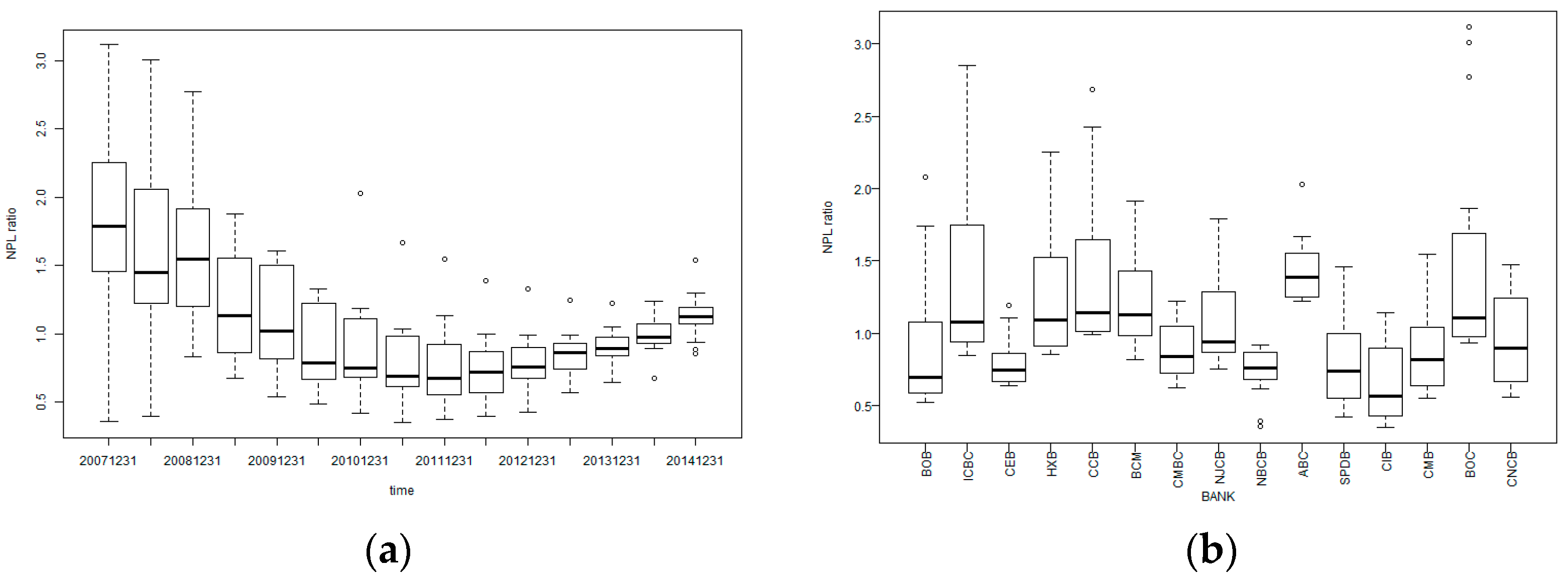
In order to answer the question as to whether the behaviors of green credit of banks affect the security of credits, we examine the relationship between CIL and NPL ratio in this section. Figure 1 presents the distribution of NPL ratio of 15 commercial banks from 2007 to 2014. As time goes on, the median of NPL ratio of 15 banks decreases first and then increases. For example, the bold horizontal line in each box decreases at first and then climbs up gradually (see Figure 1a). The heterogeneity of the NPL ratio among banks in each period exists, although it has become weak in recent periods. For each bank, heteroscedasticity is more evident, no matter the median or the dispersion (see Figure 1b).
As shown in Figure 2, NPL ratio of banks is positively related to their carbon intensity of loans, with a Pearson’s correlation coefficient of 0.32. This has well supported our argument with respect to a higher CIL and a higher NPL ratio. It is not difficult to understand the reason behind this relationship. In the background of emission reduction, companies in traditional high-emission industries are more likely to encounter bad performance due to government policy, resulting in the increase of their default risks. A commercial bank will meet with a great increase in NPL ratio to some degree if it provides more credits to such high-emission companies.
3. Model
For the further investigation on the relationship between the carbon intensity of bank loans and NPL ratio, we establish an econometric model in this section.
3.1. Variables
The issue of the determinants of NPL ratio has led many researchers to investigate possible explanations for it. According to Keeton and Morris [15], both the local economic status and the employment ratio affect the security of credits. Khemraj and Pasha [16] studied the impact factors of NPL ratio, such as deposit-to-loan ratio, inflation rate, growth rate of credits and some other similar ones. Louzis et al. [17] pointed out that the macroeconomic factors have more important influence on NPL ratio, and that the growth of GDP points to the decrease of NPL ratio to some extent. Saba [18] argued that the deposit amount of a bank is an important factor that leads to a change in the amount of NPL. Based on the panel data from 1985 to 1997, Salas and Saurina [19] concluded that economy development, management incentives of banks, and the credit portfolio have an effect upon NPL.
Similar to previous studies, we employ the NPL ratio to measure the security of bank loans in this paper. In addition to the carbon intensity of bank loans, five other indicators, two macroeconomic indicators and three microeconomic indicators, are involved in this paper (see Table 4). All of them have been considered to affect the non-performing loan ratio, according to previous literature.
In this paper, data on the non-performing loan ratio (NPLR), cost–income ratio (CI), capital adequacy ratio (CAR) and deposit-to-loan ratio (LDR) are abstracted from or calculated due to the interim statements and annual statements of China’s 15 commercial banks in 2007–2014. The statements of banks are obtained from the WIND database (Wind Info, Shanghai, China). The data of growth rate of gross domestic production (GDP) and growth rate of money supply (M2) in 2007–2014 come from the website of China’s National Bureau of Statistics (NBS), and have been adjusted to the corresponding semi-year growth rate. Apparently, the dataset forms a panel data with 15 individuals over 15 time periods. Among the six variables listed in Table 4, GDP and M2 are period individual-invariant variables, and the remaining four variables are individual time-varying variables. In consideration of the characteristics of the data used, we should carefully select an appropriate model for the subsequent empirical studies. Its details will be discussed in the following context.
3.2. Panel Data Model
Supposing that NPLR is linearly associated with CIL and the five control variables as listed in Table 4, we can form a linear model as:
where and are the intercept parameters and the slope parameters that vary across i and t, respectively. are the slope parameters that vary over t, and is the error term.
However, Equation (3) cannot be estimated, due to the fact that the available degree of freedom, 16 × 15, is less than the number of parameters, i.e., 16 × 15 × 5 + 1 × 15 × 2 + (number of parameters characterizing the distribution of ) [20]. A commonly-used solution is firstly to impose a certain structure on Equation (3) and then to make an inference.
To start with, we assume that all parameters are constant over time but can vary across individuals, which is reasonable when there are two period-variants but individual invariant variables, GDP and M2, in our data. Hence, we can rewrite Equation (3) as:
where and are the intercept parameters and the slope parameters that vary across i and t, respectively. are the slope parameters that are identical over t, and is the error term that can be characterized by an independently identically distributed random variable with mean zero and variance .
Based on Equation (4), we further impose two types of restrictions, namely:
- Model I: Both slope and intercept coefficients are the same across individuals. That is,
Model I is commonly known as a pooled model, which simply ignores the existence of heterogeneity in the panel data.
- Model II: Regression slope coefficients are identical, but intercepts are not. That is,
Unlike Model I, Model II introduces n parameters, i.e., , to allow for the effects of those unobserved factors, such as omitted variables. We can further consider two situations for in Model II. When the effects of unobserved factors are correlated to the independent variables, we call it a fixed-effects model, denoted as Model II-A in what follows. To be differential from Equation (6), we introduce a symbol of in the regression model, i.e.,
where are the effects of unobserved factors that are correlated to the independent variables. When the effects of unobserved factors are uncorrelated to the independent variables, we can separate each effect into two parts, i.e., , where is the intercept that keeps constant across i, and is the random error that can be characterized by an independently identically-distributed random variable with mean zero and variance . Thus, Equation (6) can be written as:
In this case, the effects of unobserved factors are treated as random variables that are uncorrelated to the independent variables. Therefore, we call Equation (8) a random-effects model, denoted as Model II-B.
Notice that we do not consider the situation that the intercepts are the same when the slopes are unequal, since it is seldom meaningful [20]. In what follows, we concentrate on Model I, II-A and II-B.
4. Empirical Results
For the further exploration of the relationship between NPL ratio and its determinants, we apply Model I (a pooled model), Model II-A (a fixed-effects model) and Model II-B (a random-effects model), respectively, to establish econometric models for empirical studies. To start with, data preprocessing is implemented. Since data from the China Everbright Bank (CEB) and the Agricultural Bank of China (ABC) was not available till these two banks went public in 2010, we have data of these two banks over 9 time periods and the other 15 banks over 15 time periods. In other words, our sample data is an unbalanced panel data. In order to obtain consistent estimations, we use OLS, the covariance method and generalizing OLS to estimate Model I, II-A and II-B, respectively. The estimated results of the three models are displayed in Table 5.
According to the impacts of Model I, CIL, LDR and GDP are significant with respect to NPLR, whereas the other four indicators are insignificant. The positive coefficient of CIL, i.e., 0.263, indicates that a higher level of carbon intensity of loans contributes to a higher non-performing loan ratio, which supports our argument in this paper. Therefore, low-carbon policies of bank loans are positively related to credit risk of banks. There are two kinds of causes. One is that firms with a high carbon footprint would face unexpected costs arising from potential regulatory changes in the form of caps or taxes on emissions. Therefore, in equal conditions, investing in firms with high carbon emissions in the long-term can be riskier than investing in clean firms. The other is the possibility of the falling demand for traditional high-carbon energy sources, like fossil fuels, due to the improvements in energy efficiency and the development of cleaner technologies. As governments commit funding to promote research innovation in such technologies, the potentials of technological breakthroughs can lead to a significant downside (upside) for high-carbon (low carbon) investors. This idea is similar to carbon risk, recently introduced in a paper by Oestreich and Tsiakas [21] in the context of the EU Emissions Trading Scheme. Besides, the growth of GDP prompts the increase of NPLR, while LDR has a negative association with NPLR.
In Model II-A, the impact directions of all indicators remain the same as in Model I. However, the indicator of CAR becomes significant under a 5% confidence level. If the individual heterogeneity is embodied in the intercept term, the effect of CIL upon NPLR decreases to 0.263, but is still significant. The minor change in the adjusted R2 indicates a slight improvement in the fitting performance. The estimated result of Model II-B is similar to that of Model II-A, both with four significant indicators. The effect of CIL is 0.266, slightly greater than that in Model II-A, but still smaller than that of Model I. The adjusted R2 continues to rise.
In order to find out which model is more appropriate for our data, a series of tests should be applied. Generally speaking, F-test is used to determine whether a pooled model or a fixed-effects model is suitable, and Hausman test is used to answer whether a fixed-effects or a random-effects model is appropriate. Both tests are shown in Table 6. The null hypothesis of F-test supports a pooled model, i.e., Model I in this paper. With a p-value smaller than 0.0001, we conclude that a fixed-effects model is more suitable in our case. In the Hausman test, the p-value of 0.997 does not allow for rejecting the null hypothesis. Thus, a random-effects model, i.e., Model II-B in this paper, is more appropriate. Additionally, Model II-A and Model II-B have similar fitting performances (see the adjusted R2, i.e., 0.332 and 0.351, respectively). As a consequence, we should take the results of both two models into comprehensive consideration.
Based on the above findings, at least four conclusions can be achieved.
Firstly, the carbon intensity of bank loans is positively associated with the non-performing loan ratio in banks. It is supported by both Model II-A (a fixed-effect model) and Model II-B (a random-effects model). The relationship between the two indicators is stable, regardless of models.
Besides, when looking at the two macroeconomic factors, we find out that the growth of GDP contributes to the increase of NPLR, whereas, the growth of M2 does not have a significant impact on the change of NPLR. Generally speaking, a high level of GDP corresponds to a sound macroeconomic situation. Under these circumstances, banks tend to provide easier credit policies, which leads to an increase in credit risk to some extent, or even the NPL ratio. This is consistent with the procyclicality of credit activity of banks.
Furthermore, CI has a positive but insignificant relationship with NPLR, while LDR is negatively associated with NPLR. This is in line with Kwan [22], who indicated that the risk preference, management efficiency, and risk awareness of banks are helpful for reducing the NPL ratio.
Finally, CAR has a prominent positive effect. Under the circumstance that the capital accuracy ratio is expanded, banks are likely to boost risk-taking businesses, and then suffer from an increase in NPL ratio in some degree.
5. Conclusions
According to the “Guidelines for Establishing the Green Financial System”, the environmental risk of bank credits should be under control, and the environmental risk of bank credits should be considered in the evaluation system of credit risks. In this paper, we try to provide some evidence for investigating the impact of green credits of banks upon their credit risks.
In order to measure the behaviors of green credits of banks in a quantitative way, we firstly design an indicator, named carbon intensity of loans, to describe the emission amounts associated with per unit of bank credits. We calculated the carbon intensity of loans for China’s 16 commercial banks in 29 industrial sectors from 2007 to 2014. The results showed that, for most banks, there are four industrial sectors with the characteristics of high carbon intensity, including manufacturing industry, other services, transport, storage and postal services, and wholesale, retail trade, accommodation and catering. We have successfully observed a downward trend in the carbon intensity of loans over time for a majority of banks.
Afterwards, econometric models were established to explore the relationship between the non-performing loan ratio and the carbon intensity of loans. The result of the empirical studies supports our argument that higher carbon intensity of loans will lead to a higher NPL ratio. In the overall context of emission reduction, companies in high-emission industries will encounter an increase in production cost due to government policies of carbon taxes or carbon trading, and some of them will even result in bankruptcy. On the other hand, banks will not shrink loans to such high-emission companies without the policy of green credits, and they will then meet with the increase of NPL ratio. In other words, this will result in a higher carbon intensity of loans and a higher NPL ratio. As expected, data from China’s commercial banks provides strong evidence. Accordingly, we can conclude that banks will benefit themselves from the policy of green credits. Besides, the control variables in our model give us some important insights of this issue. From the macroeconomic viewpoint, the growth of GDP contributes to the increase of the NPL ratio, while the growth of M2 does not have a significant impact. From a microeconomic viewpoint, both the management efficiency of banks and the capital adequacy ratio have important influences on the NPL ratio. The findings are consistent with previous studies.
Nevertheless, green credits in China is still in the exploring phase in practice. Based on the empirical results, we propose several policy recommendations. Firstly, banks should pay a special attention to companies in the industries of high-amount or rapid-growth emissions. Secondly, the carbon intensity of loans should be involved in the regulatory system of the China Banking Regulatory Commission (CBRC). This indicator will enable CBRC to supervise the implementation of green credits of banks, and urge the commercial banks to support the low-carbon development strategy of the government. Thirdly, concerning the standards to implement green credits, it is suggested that the amount and the change trend of carbon emissions associated with each industry should be included as an evaluation criterion of the credit risk of the industry. With an important evaluation index of environment, carbon emission should be included in the evaluation systems of green credits in different industries. According to our empirical studies, industries are different from each other in terms of their direct emission coefficient and total emission coefficient, due to their different sensitivities to the environment. However, there is a lack of evaluation criterion of environmental risks in the implementation of green credits in China. Relevant sectors in government should issue guidelines of green credits in different industries, according to the environmental impacts, technologies, and policies of different industries.
Some improvements could be made for this paper. The first one is the estimation of carbon emission in China. Recent studies indicated that the IPCC emission factors may overestimate Chinese carbon emission [23,24]. Thus, the emission factors can be updated, which is expected to make the estimation of carbon emission more accurate. Besides, the estimation accuracy of CIL can be affected by the granular level of the industry classification of banks’ credit business. Generally speaking, a more detailed classification contributes to a more accurate estimation of CIL. Therefore, it is worthy of consideration in our future work to update the CIL estimation with a more detailed industry classification.
Acknowledgments
This work is financially supported by the National Natural Science Foundation of China (grant numbers 71401192, 71420107025, 71371021, 71333014) and the National High Technology Research and Development Program of China (863 Program, grant number SS2014AA012303). The first author is partially supported by Program for Innovation Research in Central University of Finance and Economics. The second author would also like to thank the supports of the Generalized Virtual Economy Research Program of China (grant number GX2014-1007(M)) and Beijing Planning Program of Philosophy and Social Science (grant number 11JGC102).
Author Contributions
Rong Guan and Ruoen Ren conceived and designed the empirical study; Haitao Zheng performed the empirical study; Jie Hu and Qi Fang analyzed the data; Haitao Zheng contributed analysis tools; Rong Guan, Haitao Zheng and Jie Hu wrote the paper.
Conflicts of Interest
The authors declare no conflict of interest.
Appendix A
Because the industry classification in the input–output table series published by Zheng et al. [13] is different from that in China Statistical Yearbook, we provide a reconciliation in this paper. We firstly adjusted the industries in China Statistical Yearbook into 29 categories, and then merged the 42 industries from input–output tables into the 29 industries according to the same standard. To be specific, the detailed process is described as follows.
Firstly, merging of 12 industries occurred, i.e., (1) information transfer, software and information technology services; (2) finance; (3) real estate; (4) leasing and commercial services; (5) research and experimental development; (6) integrated technology services; (7) geological prospecting, administration of water, environment, and public facilities; (8) resident services and other services; (9) education; (10) health care, social insurance and social welfare; (11) culture, sports, and entertainment; (12) public administration and social organizations, into other services. Secondly, merging of 2 industries occurred, i.e., (1) transport and storage; (2) postal services, into transport, storage and postal services. Thirdly, merging of another 2 industries occurred, i.e., (1) wholesale and retail trades; (2) accommodation and catering, into wholesale, retail trade, accommodation and catering. Finally, the 29 industries were obtained (see Table A1).
In Section 2.2, we manually adjusted the industry classification and reorganized eight industries to characterize the credit structure of banks. The names of the eight industries are shown in the right-side column of Table A1.

Table A1.
Names of 29 industries and 8 industries.
| No. | Name of 29 Industries | Name of 8 Industries |
|---|---|---|
| 1 | Agriculture | Agriculture |
| 2 | Mining and washing of coal | Mining and quarrying |
| 3 | Extraction of petroleum and natural gas | |
| 4 | Mining and processing of metal ores | |
| 5 | Mining and processing of nonmetal ores and other ores | |
| 6 | Manufacture of foods and tobacco | Manufacturing |
| 7 | Manufacture of textiles | |
| 8 | Manufacture of wearing apparel, leather, fur, feather, footwear and related products | |
| 9 | Processing of timber, manufacture of furniture | |
| 10 | Printing and manufacture of paper, articles for culture, education and sports | |
| 11 | Processing of petroleum, coking, processing of nuclear fuel | |
| 12 | Manufacture of chemical products | |
| 13 | Manufacture of non-metallic mineral products | |
| 14 | Smelting and processing of metals | |
| 15 | Manufacture of metal products | |
| 16 | Manufacture of general and special purpose machinery | |
| 17 | Manufacture of transportation equipment | |
| 18 | Manufacture of electrical machinery and equipment | |
| 19 | Manufacture of computers, communication and other electronic equipment | |
| 20 | Manufacture of measuring instruments | |
| 21 | Other manufacturing | |
| 22 | Comprehensive use of waste resources | |
| 23 | Production and distribution of electric power and heat power | Utilities |
| 24 | Production and distribution of gas | |
| 25 | Production and distribution of tap water | |
| 26 | Construction | Construction |
| 27 | Transport, storage and postal services | Transport, storage and postal services |
| 28 | Wholesale, retail trade, accommodation and catering | Wholesale, retail trade, accommodation and catering |
| 29 | Other services | Other services |
Appendix B
| 2007.12 | 2008.06 | 2008.12 | 2009.06 | 2009.12 | 2010.06 | 2010.12 | 2011.06 | 2011.12 | 2012.06 | 2012.12 | 2013.06 | 2013.12 | 2014.06 | 2014.12 | Average | |
|---|---|---|---|---|---|---|---|---|---|---|---|---|---|---|---|---|
| BOB | 2.08 | 1.74 | 1.55 | 1.14 | 1.02 | 0.76 | 0.69 | 0.59 | 0.53 | 0.55 | 0.59 | 0.59 | 0.65 | 0.68 | 0.86 | 0.93 |
| ICBC | 2.85 | 2.53 | 2.38 | 1.88 | 1.61 | 1.33 | 1.08 | 0.95 | 0.94 | 0.89 | 0.85 | 0.87 | 0.94 | 0.99 | 1.13 | 1.41 |
| CEB | - | - | - | - | - | - | 0.75 | 0.67 | 0.64 | 0.64 | 0.74 | 0.80 | 0.86 | 1.11 | 1.19 | 0.82 |
| HXB | 2.25 | 2.06 | 1.82 | 1.55 | 1.50 | 1.29 | 1.19 | 0.98 | 0.92 | 0.85 | 0.88 | 0.91 | 0.90 | 0.93 | 1.09 | 1.28 |
| BCM | 1.80 | 1.83 | 1.92 | 1.51 | 1.36 | 1.22 | 1.12 | 0.98 | 0.86 | 0.82 | 0.92 | 0.99 | 1.05 | 1.13 | 1.25 | 1.25 |
| CCB | 2.69 | 2.29 | 2.43 | 1.75 | 1.55 | 1.26 | 1.14 | 1.03 | 1.14 | 1.00 | 0.99 | 0.99 | 0.99 | 1.04 | 1.19 | 1.43 |
| CMBC | 1.22 | 1.21 | 1.20 | 0.86 | 0.84 | 0.79 | 0.69 | 0.63 | 0.63 | 0.69 | 0.76 | 0.78 | 0.85 | 0.93 | 1.17 | 0.88 |
| NJCB | 1.79 | 1.39 | 1.64 | 1.36 | 1.22 | 1.07 | 0.97 | 0.85 | 0.78 | 0.75 | 0.83 | 0.92 | 0.89 | 0.93 | 0.94 | 1.09 |
| NBCB | 0.36 | 0.40 | 0.92 | 0.85 | 0.79 | 0.62 | 0.69 | 0.69 | 0.68 | 0.72 | 0.76 | 0.83 | 0.89 | 0.89 | 0.89 | 0.73 |
| PAB | 5.62 | 4.64 | 0.68 | 0.72 | 0.68 | 0.61 | 0.58 | 0.44 | 0.53 | 0.73 | 0.95 | 0.97 | 0.89 | 0.92 | 1.02 | 1.33 |
| SPDB | 1.46 | 1.22 | 1.21 | 0.90 | 0.80 | 0.62 | 0.51 | 0.42 | 0.44 | 0.53 | 0.58 | 0.67 | 0.74 | 0.93 | 1.06 | 0.81 |
| CMB | 1.54 | 1.25 | 1.11 | 0.86 | 0.82 | 0.67 | 0.68 | 0.61 | 0.56 | 0.56 | 0.61 | 0.71 | 0.83 | 0.98 | 1.11 | 0.86 |
| BOC | 3.12 | 3.01 | 2.77 | 1.86 | 1.52 | 1.20 | 1.10 | 1.00 | 1.00 | 0.94 | 0.95 | 0.93 | 0.96 | 1.02 | 1.18 | 1.50 |
| CNCB | 1.48 | 1.45 | 1.36 | 0.99 | 0.85 | 0.71 | 0.59 | 0.62 | 0.56 | 0.59 | 0.74 | 0.90 | 1.03 | 1.19 | 1.30 | 0.96 |
| CIB | 1.15 | 1.04 | 0.83 | 0.67 | 0.54 | 0.49 | 0.42 | 0.35 | 0.38 | 0.40 | 0.43 | 0.57 | 0.76 | 0.97 | 1.10 | 0.67 |
| ABC | - | - | - | - | - | - | 2.03 | 1.67 | 1.55 | 1.39 | 1.33 | 1.25 | 1.22 | 1.24 | 1.54 | 1.47 |
The non-performing loan ratio of China’s 16 commercial banks for 2007–2014.
References
- Jensen, A. Beverton and Holt life history invariants result from optimal trade-off of reproduction and survival. Can. J. Fish. Aquat. Sci. 1996, 53, 820–822. [Google Scholar] [CrossRef]
- Shahbaz, M.; Solarin, S.A.; Mahmood, H.; Arouri, M. Does financial development reduce CO2 emissions in Malaysian economy? A time series analysis. Econ. Model. 2013, 35, 145–152. [Google Scholar] [CrossRef]
- Frankel, J.A.; Romer, D. Does trade cause growth? Am. Econ. Rev. 1999, 89, 379–399. [Google Scholar] [CrossRef]
- Sadorsky, P. The impact of financial development on energy consumption in emerging economies. Energy Policy 2010, 38, 2528–2535. [Google Scholar] [CrossRef]
- Frankel, J.; Rose, A. An estimate of the effect of common currencies on trade and income. Q. J. Econ. 2002, 117, 437–466. [Google Scholar] [CrossRef]
- Ang, J.B. Economic development, pollutant emissions and energy consumption in Malaysia. J. Policy Model. 2008, 30, 271–278. [Google Scholar] [CrossRef]
- Jalil, A.; Feridun, M. Long-run relationship between income inequality and financial development in China. J. Asia Pac. Econ. 2011, 16, 202–214. [Google Scholar] [CrossRef]
- Zhang, Y.-J. The impact of financial development on carbon emissions: An empirical analysis in China. Energy Policy 2011, 39, 2197–2203. [Google Scholar] [CrossRef]
- White, M.A. Environmental finance: Value and risk in an age of ecology. Bus. Strategy Environ. 1996, 5, 198–206. [Google Scholar] [CrossRef]
- Lundgren, M.; Catasus, B. The banks’ impact on the natural environment-on the space between ‘what is’ and ‘what if’. Bus. Strategy Environ. 2000, 9, 186. [Google Scholar] [CrossRef]
- Coulson, A.B. How should banks govern the environment? Challenging the construction of action versus veto. Bus. Strategy Environ. 2009, 18, 149–161. [Google Scholar] [CrossRef]
- Allen, F.; Yago, G. Environmental finance: Innovating to save the planet. J. Appl. Corp. Financ. 2011, 23, 99–111. [Google Scholar] [CrossRef]
- Zheng, H.; Fang, Q.; Wang, C.; Wang, H.; Ren, R. China’s carbon footprint based on input-output table series: 1992–2020. Sustainability 2017, 9, 387. [Google Scholar] [CrossRef]
- Wang, H.; Wang, C.; Zheng, H.; Feng, H.; Guan, R.; Long, W. Updating input–output tables with benchmark table series. Econ. Syst. Res. 2015, 27, 287–305. [Google Scholar] [CrossRef]
- Keeton, W.R.; Morris, C.S. Why do banks’ loan losses differ? Econ. Rev. Fed. Reserv. Bank Kans. City 1987, 72, 3. [Google Scholar]
- Khemraj, T.; Pasha, S. The determinants of non-performing loans: An econometric case study of Guyana. Mpra Paper. Available online: https://mpra.ub.uni-muenchen.de/53128/1/MPRA_paper_53128.pdf (accessed on 21 April 2017).
- Louzis, D.P.; Vouldis, A.T.; Metaxas, V.L. Macroeconomic and bank-specific determinants of non-performing loans in Greece: A comparative study of mortgage, business and consumer loan portfolios. J. Bank. Financ. 2012, 36, 1012–1027. [Google Scholar] [CrossRef]
- Saba, I.; Kouser, R.; Azeem, M. Determinants of Non Performing Loans: Case of US Banking Sector. Roman. Econ. J. 2012, 44, 125–136. [Google Scholar]
- Salas, V.; Saurina, J. Credit risk in two institutional regimes: Spanish commercial and savings banks. J. Financ. Serv. Res. 2002, 22, 203–224. [Google Scholar] [CrossRef]
- Hsiao, C. Analysis of Panel Data; Cambridge University Press: Cambridge, UK, 2014. [Google Scholar]
- Oestreich, A.M.; Tsiakas, I. Carbon emissions and stock returns: Evidence from the EU Emissions Trading Scheme. J. Bank. Financ. 2015, 58, 294–308. [Google Scholar] [CrossRef]
- Kwan, S.H. Operating performance of banks among Asian economies: An international and time series comparison. J. Bank. Financ. 2003, 27, 471–489. [Google Scholar] [CrossRef]
- Zhifu, M.; Jing, M.; Dabo, G.; Yuli, S.; Zhu, L.; Yutao, W.; Kuishuang, F.; Yi-Ming, W. Pattern changes in determinants of Chinese emissions. Environ. Res. Lett. 2017. [Google Scholar] [CrossRef]
- Mi, Z.; Zhang, Y.; Guan, D.; Shan, Y.; Liu, Z.; Cong, R.; Yuan, X.-C.; Wei, Y.-M. Consumption-based emission accounting for Chinese cities. Appl. Energy 2016, 184, 1073–1081. [Google Scholar] [CrossRef]
Figure 1.
Boxplots of non-performing loan ratio (NPL). (a) NPL ratio across time; (b) NPL ratio across banks.
Figure 1.
Boxplots of non-performing loan ratio (NPL). (a) NPL ratio across time; (b) NPL ratio across banks.

Figure 2.
Scatter of carbon intensity of loans vs. nonperforming loan ratio.
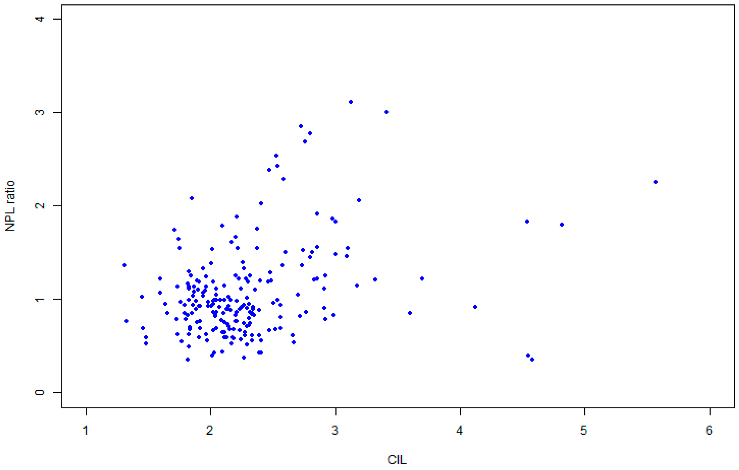
Table 1.
The direct emission coefficients (2014) and the total emission coefficients (2007–2014) of 29 industries.
Table 1.
The direct emission coefficients (2014) and the total emission coefficients (2007–2014) of 29 industries.
| No. | Industry | Direct Carbon Emission Coefficient | Total Carbon Emission Coefficient | |||||||
|---|---|---|---|---|---|---|---|---|---|---|
| 2007 | 2008 | 2009 | 2010 | 2011 | 2012 | 2013 | 2014 | |||
| 1 | Agriculture | 0.178 | 1.041 | 0.828 | 0.872 | 0.78 | 0.698 | 0.654 | 0.617 | 0.583 |
| 2 | Mining and washing of coal | 0.435 | 1.882 | 2.059 | 1.866 | 1.514 | 1.286 | 1.318 | 1.355 | 1.115 |
| 3 | Extraction of petroleum and natural gas | 0.166 | 1.102 | 0.986 | 0.961 | 0.839 | 0.64 | 0.663 | 0.644 | 0.61 |
| 4 | Mining and processing of metal ores | 0.126 | 1.366 | 1.032 | 1.151 | 0.984 | 0.845 | 0.866 | 0.859 | 0.816 |
| 5 | Mining and processing of nonmetal ores and other ores | 0.223 | 1.684 | 1.281 | 1.504 | 1.328 | 1.037 | 1.061 | 1.017 | 0.952 |
| 6 | Manufacture of foods and tobacco | 0.079 | 1.312 | 0.952 | 1.131 | 0.996 | 0.864 | 0.784 | 0.734 | 0.667 |
| 7 | Manufacture of textiles | 0.075 | 1.56 | 1.155 | 1.305 | 1.139 | 1.004 | 0.92 | 0.884 | 0.809 |
| 8 | Manufacture of apparel, leather and related products | 0.03 | 1.324 | 1.008 | 1.153 | 1.022 | 0.885 | 0.81 | 0.765 | 0.699 |
| 9 | Processing of timber, manufacture of furniture | 0.066 | 1.362 | 1.072 | 1.262 | 1.139 | 0.959 | 0.881 | 0.85 | 0.79 |
| 10 | Printing and manufacture of paper, education and sports | 0.139 | 1.71 | 1.356 | 1.609 | 1.457 | 1.265 | 1.106 | 0.995 | 0.871 |
| 11 | Processing of petroleum, coking, nuclear fuel | 0.514 | 2.219 | 1.784 | 2.006 | 1.612 | 1.354 | 1.332 | 1.299 | 1.225 |
| 12 | Manufacture of chemical products | 0.413 | 2.493 | 1.81 | 2.134 | 1.941 | 1.713 | 1.602 | 1.535 | 1.472 |
| 13 | Manufacture of non-metallic mineral products | 1.203 | 4.257 | 3.167 | 3.74 | 3.403 | 2.957 | 2.671 | 2.514 | 2.334 |
| 14 | Smelting and processing of metals | 0.409 | 2.04 | 1.627 | 1.963 | 1.775 | 1.566 | 1.495 | 1.472 | 1.389 |
| 15 | Manufacture of metal products | 0.036 | 1.559 | 1.24 | 1.452 | 1.095 | 1.157 | 1.112 | 1.084 | 1.02 |
| 16 | Manufacture of general and special purpose machinery | 0.027 | 1.427 | 1.123 | 1.299 | 1.013 | 1.014 | 0.976 | 0.957 | 0.905 |
| 17 | Manufacture of transportation equipment | 0.022 | 1.376 | 1.091 | 1.187 | 1.093 | 0.991 | 0.955 | 0.922 | 0.869 |
| 18 | Manufacture of electrical machinery and equipment | 0.011 | 1.595 | 1.249 | 1.445 | 1.132 | 1.164 | 1.125 | 1.095 | 1.028 |
| 19 | Manufacture of computers and other electronic equipment | 0.005 | 1.329 | 1.054 | 1.162 | 0.968 | 0.913 | 0.851 | 0.837 | 0.8 |
| 20 | Manufacture of measuring instruments | 0.007 | 1.409 | 1.091 | 1.211 | 1.048 | 0.979 | 0.927 | 0.912 | 0.859 |
| 21 | Other manufacturing | 0.052 | 1.378 | 1.099 | 1.093 | 0.878 | 0.775 | 1.056 | 0.727 | 0.564 |
| 22 | Comprehensive use of waste resources | 0.028 | 0.182 | 0.168 | 0.249 | 0.329 | 0.306 | 0.292 | 0.296 | 0.306 |
| 23 | Production and distribution of electric power and heat power | 0.046 | 1.233 | 1.213 | 1.189 | 1.038 | 0.766 | 0.92 | 0.872 | 0.714 |
| 24 | Production and distribution of gas | 0.083 | 1.479 | 1.319 | 1.054 | 0.878 | 0.682 | 0.707 | 0.681 | 0.675 |
| 25 | Production and distribution of tap water | 0.023 | 0.925 | 0.803 | 0.801 | 0.69 | 0.607 | 0.631 | 0.612 | 0.558 |
| 26 | Construction | 0.119 | 2.111 | 1.636 | 1.791 | 1.634 | 1.45 | 1.343 | 1.282 | 1.199 |
| 27 | Transport, storage and postal services | 1.421 | 3.013 | 2.698 | 2.717 | 2.511 | 2.288 | 2.299 | 2.263 | 2.132 |
| 28 | Wholesale, retail trade, accommodation and catering | 0.254 | 1.138 | 0.923 | 0.924 | 0.805 | 0.739 | 0.692 | 0.659 | 0.616 |
| 29 | Other services | 0.516 | 1.734 | 1.482 | 1.425 | 1.272 | 1.168 | 1.111 | 1.057 | 0.98 |
Unit: ton/ten thousand yuan.
Table 2.
Carbon emissions in eight industries and carbon intensity of loans of the Shanghai Pudong Development Bank (SPDB) for 2007–2014.
Table 2.
Carbon emissions in eight industries and carbon intensity of loans of the Shanghai Pudong Development Bank (SPDB) for 2007–2014.
| Period | Carbon Emission of Industry (10 Thousand Tons) | Carbon Intensity of Loans (Tons/10 Thousand) | |||||||
|---|---|---|---|---|---|---|---|---|---|
| 1 | 2 | 3 | 4 | 5 | 6 | 7 | 8 | ||
| 2007.12 | 16 | 95 | 10,288 | 193 | 383 | 832 | 558 | 1249 | 3.09 |
| 2008.06 | 16 | 139 | 10,712 | 269 | 407 | 901 | 535 | 1184 | 2.85 |
| 2008.12 | 19 | 172 | 12,109 | 338 | 443 | 1081 | 564 | 1243 | 2.83 |
| 2009.06 | 25 | 200 | 15,169 | 257 | 609 | 1956 | 819 | 1429 | 2.91 |
| 2009.12 | 24 | 187 | 14,059 | 233 | 582 | 1425 | 672 | 1509 | 2.56 |
| 2010.06 | 22 | 200 | 13,470 | 252 | 605 | 1512 | 676 | 1681 | 2.27 |
| 2010.12 | 33 | 221 | 15,228 | 265 | 623 | 1703 | 766 | 1935 | 2.29 |
| 2011.06 | 35 | 217 | 14,372 | 179 | 598 | 1661 | 788 | 1948 | 2.03 |
| 2011.12 | 42 | 235 | 16,358 | 186 | 669 | 1688 | 943 | 1792 | 2.09 |
| 2012.06 | 45 | 284 | 18,106 | 237 | 691 | 1829 | 1068 | 1726 | 2.17 |
| 2012.12 | 55 | 325 | 19,589 | 219 | 742 | 1898 | 1192 | 1813 | 2.19 |
| 2013.06 | 55 | 337 | 19,725 | 195 | 945 | 1899 | 1332 | 3637 | 2.23 |
| 2013.12 | 67 | 357 | 19,541 | 194 | 1016 | 1834 | 1495 | 5914 | 2.27 |
| 2014.06 | 69 | 319 | 17,094 | 153 | 1068 | 1806 | 1608 | 6211 | 1.98 |
| 2014.12 | 74 | 334 | 17,324 | 157 | 1076 | 1761 | 1755 | 7022 | 1.94 |
Note: The number of 1–8 correspond to 8 industries, i.e., 1—Agriculture; 2—Mining and quarrying; 3—Manufacturing; 4—Utilities; 5—Construction; 6—Transport, storage and postal services; 7—Wholesale, retail trade, accommodation and catering; and 8—Other services.
Table 3.
Carbon intensity of loans (CIL) for China’s 16 commercial banks for 2007–2014 (ton/ ten thousand Yuan).
Table 3.
Carbon intensity of loans (CIL) for China’s 16 commercial banks for 2007–2014 (ton/ ten thousand Yuan).
| Bank | 2007.12 | 2008.06 | 2008.12 | 2009.06 | 2009.12 | 2010.06 | 2010.12 | 2011.06 | 2011.12 | 2012.06 | 2012.12 | 2013.06 | 2013.12 | 2014.06 | 2014.12 | Average |
|---|---|---|---|---|---|---|---|---|---|---|---|---|---|---|---|---|
| BOB | 1.85 | 1.71 | 1.75 | 1.74 | 1.45 | 1.32 | 1.46 | 1.48 | 1.48 | 1.77 | 1.91 | 2.11 | 2.09 | 1.83 | 1.79 | 1.72 |
| ICBC | 2.73 | 2.52 | 2.47 | 2.21 | 2.16 | 1.94 | 1.86 | 1.64 | 1.8 | 1.88 | 1.85 | 2.05 | 2.02 | 1.82 | 1.82 | 2.05 |
| CEB | - | - | - | - | - | - | 2.11 | 2.02 | 2.11 | 2.27 | 2.31 | 2.31 | 2.32 | 2.04 | 2.02 | 2.17 |
| HXB | 5.57 | 3.19 | 3 | 2.85 | 2.82 | 2.48 | 2.46 | 2.21 | 2.25 | 2.33 | 2.39 | 2.34 | 2.29 | 2 | 1.96 | 2.68 |
| BCM | 4.82 | 4.54 | 2.86 | 2.6 | 2.57 | 2.28 | 2.24 | 2.02 | 2.02 | 2.03 | 2.07 | 2.11 | 2.05 | 1.87 | 1.84 | 2.53 |
| CCB | 2.76 | 2.59 | 2.54 | 2.37 | 2.37 | 2.2 | 2.11 | 1.86 | 1.96 | 2.03 | 2.03 | 2.11 | 2.08 | 1.94 | 1.89 | 2.19 |
| CMBC | 3.7 | 3.32 | 2.49 | 2.21 | 2.04 | 1.72 | 1.84 | 1.74 | 1.83 | 1.91 | 1.91 | 2.09 | 2.1 | 1.92 | 1.81 | 2.18 |
| NJCB | 2.09 | 2 | 1.75 | 1.31 | 1.6 | 1.59 | 1.76 | 1.65 | 1.8 | 1.89 | 1.82 | 2.14 | 2.13 | 1.91 | 1.86 | 1.82 |
| NBCB | 4.58 | 4.55 | 4.12 | 3.6 | 2.92 | 2.66 | 2.56 | 2.04 | 2.18 | 2.31 | 2.2 | 2.35 | 2.34 | 2.23 | 2.16 | 2.85 |
| PAB | 3.21 | 3.13 | 3.38 | 2.52 | 2.4 | 2.24 | 2.33 | 2.14 | 2.12 | 2.19 | 2.18 | 1.93 | 1.79 | 1.52 | 1.47 | 2.30 |
| SPDB | 3.09 | 2.85 | 2.83 | 2.91 | 2.56 | 2.27 | 2.29 | 2.03 | 2.09 | 2.17 | 2.19 | 2.23 | 2.27 | 1.98 | 1.94 | 2.38 |
| CMB | 3.1 | 2.92 | 2.91 | 2.76 | 2.71 | 2.47 | 2.52 | 2.33 | 2.33 | 2.41 | 2.39 | 2.29 | 2.2 | 1.89 | 1.83 | 2.47 |
| BOC | 3.13 | 3.41 | 2.79 | 2.98 | 2.74 | 2.4 | 2.36 | 2.05 | 2.16 | 2.27 | 2.3 | 2.56 | 2.5 | 2.3 | 2.3 | 2.55 |
| CNCB | 3 | 2.8 | 2.74 | 2.53 | 2.33 | 2.15 | 2.18 | 1.97 | 1.97 | 2.13 | 2.13 | 2.14 | 2.14 | 1.91 | 1.82 | 2.26 |
| CIB | 3.17 | 2.7 | 2.98 | 2.15 | 2.67 | 1.82 | 2.39 | 1.82 | 2.27 | 2.02 | 2.4 | 2.24 | 2.21 | 1.98 | 1.9 | 2.31 |
| ABC | - | - | - | - | - | - | 2.41 | 2.2 | 2.22 | 2.26 | 2.27 | 2.31 | 2.22 | 1.97 | 2.02 | 2.21 |
| std. | 0.99 | 0.77 | 0.73 | 0.54 | 0.42 | 0.37 | 0.3 | 0.23 | 0.22 | 0.18 | 0.19 | 0.15 | 0.16 | 0.17 | 0.17 | 0.37 |
Table 4.
Variable declaration.
| Type | Name | Meaning |
|---|---|---|
| dependent variable | NPLR | non-performing loan ratio |
| independent variable | CIL | carbon intensity of loan |
| control variable | CI | cost–income ratio |
| LDR | deposit-to-loan ratio | |
| CAR | capital adequacy ratio | |
| GDP | growth rate of gross domestic production | |
| M2 | growth rate of money supply |
Table 5.
The estimated coefficients of Model I, II-A and II-B.
| Variables | Model I | Model II-A | Model II-B |
|---|---|---|---|
| CIL | 0.269 *** | 0.263 *** | 0.266 *** |
| (4.32) | (4.618) | (4.778) | |
| CI | 0.304 | 0.71 | 0.68 |
| (0.452) | (0.902) | (0.916) | |
| CAR | 0.013 | 0.030 ** | 0.027 ** |
| (1.043) | (2.447) | (2.343) | |
| LDR | −7.794 *** | −9.094 *** | −8.815 *** |
| (−6.344) | (−5.717) | (−6.03) | |
| GDP | 3.437 ** | 3.089 ** | 3.110 ** |
| (2.102) | (2.084) | (2.156) | |
| M2 | 0.232 | 0.298 | 0.287 |
| (0.292) | (0.453) | (0.443) | |
| Constant | 3.036 *** | - | 3.188 *** |
| (5.255) | - | (4.982) | |
| Adjusted R2 | 0.290 | 0.332 | 0.351 |
Note: *** p < 0.01; ** p < 0.05.
Table 6.
Model selection.
| F-Test | Hausman-Test | |
|---|---|---|
| df | 14,192 | 6 |
| Statistics | F = 8.261 | H = 0.559 |
| p-value | < 0.0001 | 0.997 |
| H0 | Model I | Model II-B |
| H1 | Model II-A | Model II-A |
© 2017 by the authors. Licensee MDPI, Basel, Switzerland. This article is an open access article distributed under the terms and conditions of the Creative Commons Attribution (CC BY) license (http://creativecommons.org/licenses/by/4.0/).
Share and Cite
MDPI and ACS Style
Guan, R.; Zheng, H.; Hu, J.; Fang, Q.; Ren, R. The Higher Carbon Intensity of Loans, the Higher Non-Performing Loan Ratio: The Case of China. Sustainability 2017, 9, 667. https://doi.org/10.3390/su9040667
AMA Style
Guan R, Zheng H, Hu J, Fang Q, Ren R. The Higher Carbon Intensity of Loans, the Higher Non-Performing Loan Ratio: The Case of China. Sustainability. 2017; 9(4):667. https://doi.org/10.3390/su9040667
Chicago/Turabian StyleGuan, Rong, Haitao Zheng, Jie Hu, Qi Fang, and Ruoen Ren. 2017. "The Higher Carbon Intensity of Loans, the Higher Non-Performing Loan Ratio: The Case of China" Sustainability 9, no. 4: 667. https://doi.org/10.3390/su9040667
Note that from the first issue of 2016, this journal uses article numbers instead of page numbers. See further details here.