
Modeling the Relative Contributions of Land Use Change and Harvest to Forest Landscape Change in the Taihe County, China

1
Key Laboratory of Land Surface Pattern and Simulation, Institute of Geographic Sciences and Natural Resources Research, Chinese Academy of Sciences, Beijing 100101, China
2
University of Chinese Academy of Sciences, Beijing 100049, China
*
Author to whom correspondence should be addressed.
Sustainability 2017, 9(5), 708; https://doi.org/10.3390/su9050708
Submission received: 22 January 2017
/
Revised: 25 April 2017
/
Accepted: 26 April 2017
/
Published: 28 April 2017
(This article belongs to the Section Environmental Sustainability and Applications)
Abstract
:Forests are under pressure from land use change due to anthropogenic activities. Land use change and harvest are the main disturbances of forest landscape changes. Few studies have focused on the relative contributions of different disturbances. In this study, we used the CA-Markov model, a land-use change model, coupled with a forest landscape model, LANDIS-II, to simulate dynamic change in Taihe County, China, from 2010 to 2050. Scenarios analysis was conducted to quantify the relative contributions of land use change and harvest. Our results show that forestland and arable land will remain the primary land-use types in 2050, whereas the built-up land will sprawl drastically. Land use change and harvest may result in the significant loss of forest area and changes in landscape structure. The simulated forest area will increase by 16.2% under the no disturbance scenario. However, under harvest, forest conversion, and integrated scenario, the area will be reduced by 5.2%, 16.5%, and 34.9%, respectively. The effect of harvest is gradually enhanced. The land use change will account for 60% and harvest will account for 40% of forest landscape change in 2050, respectively. Our results may benefit from the integration of regional forest management and land-use policy-making, and help to achieve a trade-off between economy and ecological environment.
1. Introduction
Forests, one of the most important terrestrial ecosystems, cover almost 31% of the world, and significantly contribute not only to global wood production, but also to crucial ecosystem services like CO2 sequestration, soil protection, and climate change effects mitigation [1,2]. Unfortunately, a large amount of evidence has shown that in recent years, forest loss has occurred more commonly than forest gain, although the characteristics of forest change differ, depending on the region and the driving forces [3,4,5]. With the rapid increase in global population, the demand for land resources has increased continually, which may result in substantial pressure being placed on forests by anthropogenic activities [6,7]. In terms of diverse natural and anthropogenic disturbances, land use change and harvest are the two most remarkable and direct factors affecting the forest landscape [8,9,10]. Additionally, these anthropogenic disturbances are the most effective way for achieving regional forest management objectives.
In general, land use change and harvest appear at a local and regional scale [11]. Many studies have been conducted to investigate forest changes in response to disturbances of land use change and harvest on a regional and landscape scale [7,12]. For example, Drummond and Loveland [3] used remote-sensing data, statistical sampling, and change-detection methods to study regional forest changes in the eastern United States. They found that even though agricultural land use had declined, which may be beneficial for forest recovery, forest-cover loss caused by timber cutting cycles, urbanization, and other land use demands, had occurred. Scheller and Mladenoff [13] used a forest landscape model to estimate the combined effects of climate change, common disturbances, and species migrations on regional forests under various scenarios. They found that these important spatially interactive processes affected the forest composition and aboveground live biomass of northern Wisconsin forests, resulting in the loss of species and biomass. Thompson et al. [14] used the LANDIS-II model to evaluate how the forest composition dynamics were affected by land use and climate change in Massachusetts, USA. They found that land use changed the forestland into developed uses. In addition, studies of relative contributions have also been extensively investigated at different scales. For example, Abood et al. [15] calculated the relative contributions of the logging, fiber, oil palm, and mining industries to the forest loss in Indonesia. They compared the magnitudes of forest and carbon loss and that remaining within different industrial concessions. Fang et al. [16] explored the relative contributions of forest expansion and forest growth to forest biomass carbon sinks in East Asia. At the stand scale, Pallett et al. [17] designed five trials to demonstrate the relative contributions of different factors associated with productivity gains. They found that silvicultural treatments were the largest contributors to productivity differences. These studies hold lessons for the study of forest disturbances. In terms of our study area, land use change and harvest have contributed significantly to forest losses. However, much uncertainty remains over the relative contributions to forest losses at present or in the near future. Therefore, we used a scenario analysis to quantify the relative contributions of land use change and harvest to forest landscape change.
Spatial simulation models are efficient tools for quantitatively simulating and exploring landscape change, especially under different disturbance scenarios [18]. Generally, studies of land use change and harvesting are relatively independent, and different models can simulate the effects on the forest landscape. In terms of land use change, the CA (Cellular Automata)-Markov model is a stochastic model based on a transition matrix, which has been widely used in studies of land cover change on various spatial scales [19,20,21]. LANDIS-II is a forest landscape disturbance and succession model that operates on landscapes mapped out as cells [22,23]. This model was specifically designed to address the effect of harvesting and natural disturbances (fire, wind, and insects) on forests, and has been widely used in regional forest management [6,24]. These two models have the advantages of being coupled to deal with integrated effects on forest landscapes. In addition, by embedding the access point between the two models, the synthesis simulation can be realized.
Currently, China has the fastest growing planted forests in the world, which account for around 23% the total forest area in the world [1]. Especially in the southern region, the plantations occupy 63% of the total forested area throughout China [25]. These forests play an important role in regional wood production, biodiversity protection, ecosystem service provision, and economic development. However, with increasing demands for land and timber, the threat derived from land use change and harvest is increasingly serious. Taihe County is a typical forested region in southern China, which includes almost all the major forest types. A large area of plantations distributed in this area is representative of southern China. Studying the effects of land use change and harvest on the forest landscape may benefit regional forest management, and the results can also be extended to other areas in southern China. Therefore, in this study, we used CA-Markov, a land-use change model, coupled with a forest landscape model, LANDIS-II, to simulate dynamic change in the forest landscape in response to the disturbances of land use change and harvest in Taihe County, China, from 2010 to 2050. Scenario analysis was conducted to quantify the relative contributions of land use change and harvest to forest landscape change. Our objectives of this study were: (1) to simulate forest landscape changes driven by land use change and harvest; and (2) to quantify the relative contributions of land use change and harvest to forest landscape change. The quantitative simulations help illustrate the driving forces of forest structure change, integrating the regional forest management strategy and land use planning into the near future.
2. Materials and Methods
2.1. Study Area
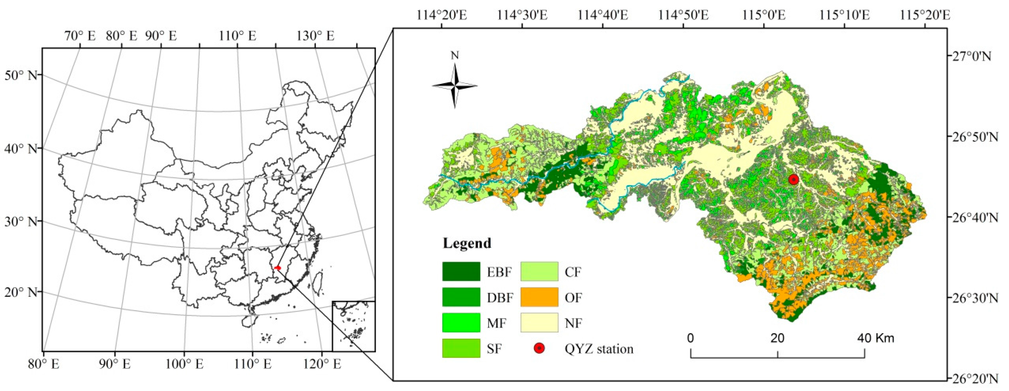
Taihe County (26.45°–26.98°N, 114.95°–115.33°E) is located in the south-central Jiangxi Province of southern China (Figure 1). It is a typical hilly red soil region of southern China, which is a major component of the Jitai Basin with a rolling hilly terrain. The total area is 266,700 ha, and the forest area accounts for 61.2% of the total area. This area has a subtropical monsoon climate with mild winters (with a mean January temperature of 6.5 °C) and warm summers (with a mean July temperature of 29.7 °C), and the average annual temperature is 18.6 °C. The average annual precipitation is 1370 mm, the majority of which (approximately 60%) falls between March and June [26]. There are six main land use types in our study area, including forestland, arable land, grass land, built-up land, unused land, and water body. The original vegetation was a subtropical evergreen broad-leaved forest, but due to degradation and long-term human disturbances, the forest landscape has been converted into subtropical coniferous plantations. The coniferous plantations cover 73,292 ha, which accounts for 44.9% of the total forested area according to forestry resource survey data from Jiangxi Province in 2009 [27]. There are 18 dominant species within our study area, including masson pine (Pinus massoniana), slash pine (Pinus elliottii), Chinese fir (Cunninghamia lanceolata), Chinese weeping cypress (Cupressus funebris), camphor tree (Cinnamomum camphora), zhennan (Phoebe zhennan), crenate gugertree (Schima superba), beautiful sweetgum (Liquidambar formosana), Chinese sassafras (Sassafras tzumu), eyer evergreenchinkapin (Castanopsis eyrei), myrsinaleaf oak (Cyclobalanopsis gracilis), fortune chinabells (Alniphyllum fortunei), farges evergreenchinkapin (Castanopsis fargesii), longpeduncled alder (Alnus cremastogyne), faber oak (Quercus fabri), shinybark birch (Betula luminifera), chinaberry (Melia azedarach), and poplar (Populus deltoides).
To investigate changes in the interior structure of the forest landscape, five representative forest types were chosen, including evergreen broad-leaved forests (EBF), deciduous broad-leaved forests (DBF), masson pine forests (MF), slash pine forests (SF), and Chinese fir forests (CF). Moreover, some other forest (OF) types were not considered in our simulation, such as bamboo forests and economic forests. Bamboo is a herbaceous plant and there is a big difference in the physiological features and plant growth between bamboo and these other dominant tree species. For the economic forests, most of them are cash crops, such as orange trees and tea bushes. The economic forests were not considered because they are characterized by specific management and a peculiar kind of forest cover. The distribution of different forest types is shown in Figure 1. The coniferous forests were distributed in the lower mountain areas below 1000 m. The broad-leaved forests were mainly spread over the lower hills, with elevations between 100 and 900 m. In addition, there is a long-term ecological observation station located in this area, called Qianyanzhou Experiment Station for Comprehensive Development of Natural Resources in the Red Earth Hilly Area (Figure 1). This station was founded by the Chinese Academy of Sciences in 1982. Long-term observational data, such as climate (temperature, precipitation, photosynthetically active radiation (PAR), and CO2 concentration), soil (water hold capacity and soil type), and species life history attributes are an important and credible data source for our study.
2.2. Modeling Framework
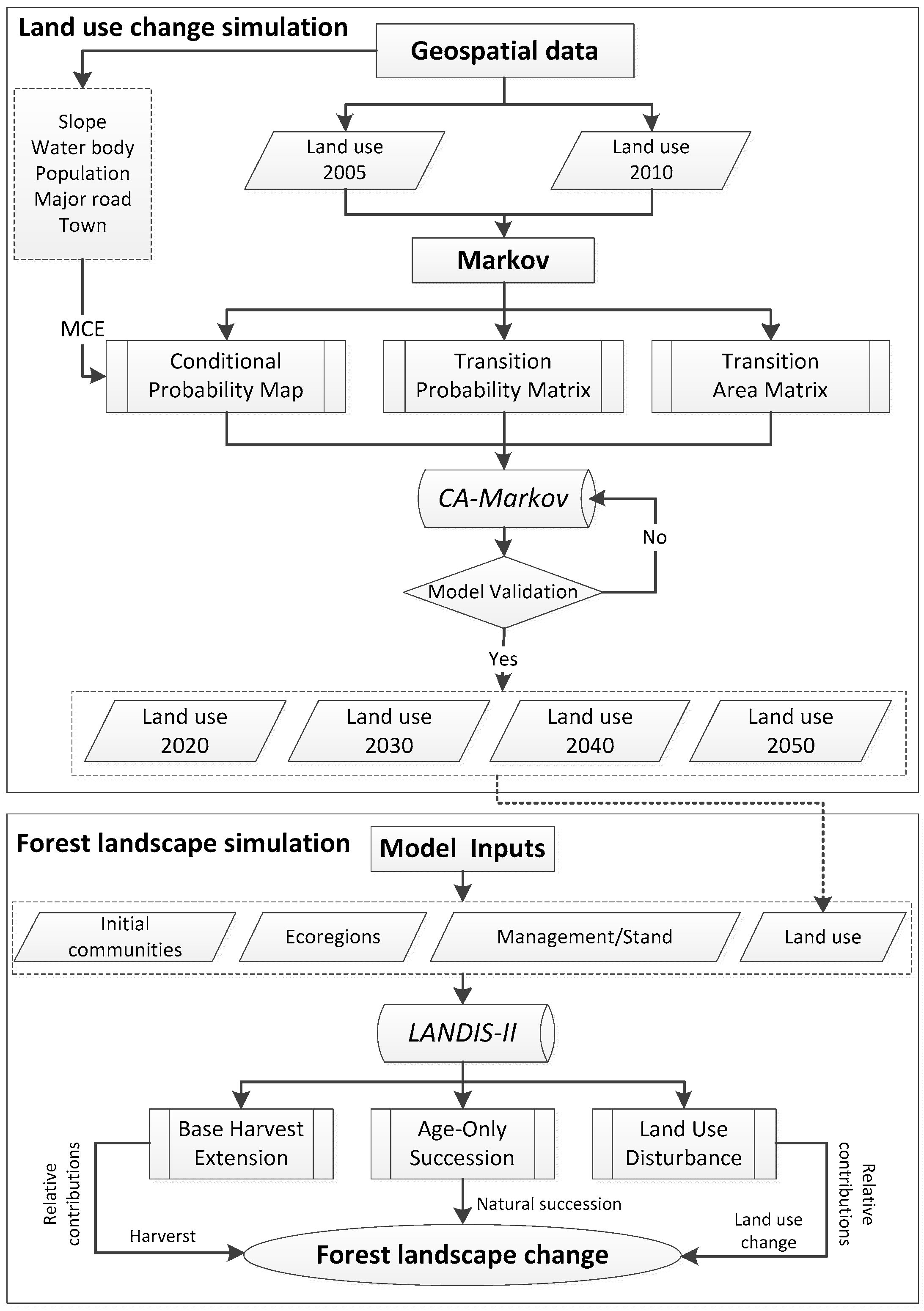
We used the CA-Markov model and LANDIS-II model to simulate the effects of land use change and harvest on the forest landscape. A coupled modeling framework was built to achieve the research objectives (Figure 2). The CA-Markov model was used to simulate and predict land use change under the current scenario in the near future (2020–2050). The outputs of the land use change simulation can help identify the conversion of forest to non-forest land cover. Additionally, these maps were used as inputs for the LANDIS-II model to simulate the effects of land use change on forests (e.g., forestland converted to built-up land or farmland). The LANDIS-II was used to simulate the forest landscape change under natural succession, land use change, and harvest. The Age-Only Succession extension, the Base Harvest extension, and Land Use disturbance for the LANDIS-II model were used to simulate the independent and integrated effects, respectively. Finally, the relative contributions of land use change and harvest to forest landscape change were calculated by these independent and integrated simulation results.
2.3. Land-Use Change Simulation
We used the CA-Markov model to conduct the land-use change simulation in our study. The observed land-use datasets in 2005 and 2010 were obtained from the land and resources survey of the department of land and resources of Jiangxi Province, China. The spatial resolution of the land use datasets was 100 m, and this resolution was also used for the future simulation. These geospatial data were used as the original inputs, and for determining the transition rules for predicting the land-use pattern in the near future. The CA-Markov model incorporates the theories of the Markov chain and CA, and focuses on the quantity of predictions for land use changes [28]. The Markov model can explain the quantification of conversion states between land use types and predict the geographical characteristics. However, the model lacks spatial parameters and does not express changes in spatial extents [19]. The CA model focuses mainly on the local interactions of cells with distinct temporal and spatial coupling features and the powerful computing capability of space, which is especially suitable for dynamic simulation and display [21]. Through the integration of methods, the CA-Markov model can achieve a better simulation for temporal and spatial patterns of land use changes [21]. The CA-Markov module in IDRISI 17.0 software [29] was used to simulate and predict changes in the future spatial-temporal pattern of land use in Taihe County. There are several steps in the simulation (Figure 2), and the specific process is as follows:
- (1)
- Calculated the transition matrix using Markov. The transition area matrix and transition probability matrix were obtained through the Markov module, which were derived from the land use maps in 2005 and 2010.
- (2)
- Generated conditional probability maps. The Multi-Criteria Evaluation (MCE) module in IDRISI was used to generate the conditional probability maps for each land use type [30]. In this study, many factors were considered, such as the slope, distance to the water body, population, major road, and town center, as well as their influence on each land use type. Then, these maps were standardized and unified onto one conditional map for the CA-Markov simulation input.
- (3)
- Simulated land use using the CA-Markov model. First, CA filters were determined as a standard 5 × 5 contiguity filter in this study. Second, the precision of the simulation was tested. The spatial consistency was checked using the overall Kappa spatial correlation statistic between the observed 2010 and simulated 2010 land use datasets. The Kappa index is the summary statistics [31]. The actual and simulated land use maps in 2010 are shown in Figure 3. The results showed that the spatial pattern of land use type was consistent. The overall Kappa statistic was 0.9176, which was well above 0.80, demonstrating that the transition rules could be used to predict the spatial pattern of land use in our study area [32]. Finally, the starting point and number of iterations were decided. We took the land use map from 2010 as a starting point and selected 10 CA iterations to simulate the predicted spatial pattern of land use in 2020. Then, the 2020 land use map was used as the basis to simulate the predicted land use pattern in 2030 with 10 further CA iterations, and so on, until the year 2050.
2.4. Forest Landscape Simulation
We used the LANDIS-II model as the core to simulate the effects of land use change and harvest on the forest landscape. The LANDIS-II model is a cell-based spatially dynamic forest landscape model of disturbance, succession, and management [22,33]. It can simulate forest dynamics by tracking the age cohorts of the species (cohorts of trees within the same age range) [34,35]. Considering the LANDIS model, forest landscape change is driven by species life history attributes, the species establishment probability (SEP), the aboveground net primary production (ANPP), disturbances, and spatial heterogeneity [22]. Many extensions have been developed and grouped into succession and disturbance, and they are extensively applied in forest landscape research [14,23,24,36,37]. In this study, various experimental designs were conducted to simulate disturbances and succession. The Age-Only Succession extension was used to simulate the forest landscape distribution under natural succession, and the Base Harvest extension was used to address the effects of harvest on forest landscapes. In terms of the effects of land use change, we used the outputs from the CA-Markov model as the inputs for LANDIS-II. We extracted the area in which land use change appears from the predicted land use maps in 2020, 2030, 2040, and 2050. Once the land use change is assigned to a site, the land cover and trees of this site will be removed and cannot be simulated at this time point. We overlapped the land use map with the initial community map, assigning the converted sites to non-active in the simulation. Based on this, we could determine the effect of land use disturbances on the forest landscape.
For parameterization, the inputs for LANDIS-II include spatial data (initial communities map, ecoregions map, management map, stand map, and land use map) and non-spatial data (species life history attributes, ANPP, and SEP). The spatial inputs were raster data with a 100 m cell size, and this resolution was also used for scenario modeling. The initial communities map was derived from the survey data of the forestry resource of Jiangxi Province in 2009. This map was divided into 73 communities, which indicates the distribution and age of the tree species and forest type at the beginning of the simulation. For the harvest experiment design, the forest landscape was divided into management areas and harvest stands, which had a hierarchy of areas for harvesting. The management areas were collections of stands for the application of specific harvesting prescriptions, and were based on the classification of forest types. In this experiment, CF were defined prior to harvest simulation, and then MF, SF, DBF, and EBF were also defined. The harvest prescription for our study was consistent with the contemporary status of the forest management policy. According to the regulations, the logging cycle was designed with a time period of 10 years, and the harvest area was set as 10% for different forest management areas. In addition, there is a limitation in the harvest simulation. The harvest events occurred until the tree species reached their mature age. We defined the mature age based on the forest management regulations: CF (>21), MF and SF (>26), and DBF and EBF (>41). The ecoregion map was also divided into five ecoregions, which were based on relatively homogeneous geomorphic forms (Figure 4). In detail, the ecoregions were: (1) non-forest land; (2) low hills (below 100 m); (3) medium hills (100–250 m); (4) high hills (250–500 m); and (5) mountains (above 500 m). Ecoregion 1 was inactive in the simulation. Finally, the land use maps were derived from the results of the CA-Markov model. The parameters of the species life history attributes were mainly compiled from the literature, plot investigations, and consultations with local forestry experts [38,39] (Table 1).
The results of ANPP and SEP for each species were calculated by version 5.1 of the PnET-II (Los Alamos National Laboratory, Los Alamos, NM, USA) model. For parameterization, climatic data were the key inputs, and the temperature and precipitation were compiled from ten-year (2001–2011) averages, which were obtained from the QYZ ecological station. The water holding capacity (WHC), PAR, and CO2 concentration were also derived from the observation station. The foliar nitrogen concentration is a crucial parameter in the process of the ANPP calculation, leading to changes in the maximum net photosynthetic rate. This variable was referenced from the publication by Yu et al. [40]. Some important parameters for each species were acquired from the published literature, including the minimum temperature for photosynthesis [39,41], optimum temperature for photosynthesis [39,42], and water use efficiency (WUE) [43]. In addition, some fixed parameters were taken from the literature [44,45,46,47,48].
2.5. Quantifying the Relative Contributions of Land Use Change and Harvest
The scenario analysis method was applied to quantify the relative contributions of land use change and harvest to forest landscape change in the simulation. First, we assumed that the forest landscape was only under the influence of land use change and harvest. The forest area was used as a quantitative indicator to describe variations in the landscape. In this study, four scenarios were presumed and simulated: (1) the natural forest landscape succession without disturbances; (2) the forest landscape succession with only land use change disturbance; (3) the forest landscape succession with only harvest; and (4) the forest landscape succession with both land use change and harvest disturbances (the integrated scenario). The forest landscape under different scenarios was controlled by adjusting the respective parameter in the LANDIS-II model. Following this, the relative effects of land use change and harvest were quantified. The processes are as follows:
where AN is the simulated forest area with no disturbance; AL is the simulated forest area under the scenario with land use change; AH is the simulated forest area under the scenario with harvest; AH+L is the simulated forest area under the scenario with both harvest and conversion; ΔAL is the forest area variation with land use change; ΔAH is the forest area variation with harvest; ΔAH+L is the forest area variation with both harvest and conversion; and ηL and ηH are the contributions of land use change and harvest to the forest landscape, respectively.
3. Results
3.1. Land-Use Change Simulation
In terms of the spatial pattern, the results of the simulation show that the holistic spatial pattern of land use will not change significantly during the period 2010–2050 (Figure 5). The forestland and arable land will remain the primary land use type to 2050. However, the built-up land will sprawl drastically and intensively, which will intrude into arable land, forestland, and unused land. In particular, the unused land will be almost entirely invaded in the year 2050. The main concentration of the town expansion is in the center of the study area, which has been sprawling northward. The forest landscape change is more concerning in this study. The results show that the land use change mainly occurs on the border of the arable land, which is located on gentle slope terrain, such as in Ecoregion 2. In terms of the variation of quantity, the area of forestland affected by the land use change will decrease by 7146 ha, showing a 4.4% loss of the forest area during the period 2010–2050. The amount of unused land area will decline more significantly. The unused land area will decrease from 2218 to 107 ha during 2010–2050, reducing by 95.2%. The built-up land and arable land will increase by 32.2% (4752 ha) and 10.8% (7568 ha) during the simulation, respectively.
3.2. Forest Landscape Simulation
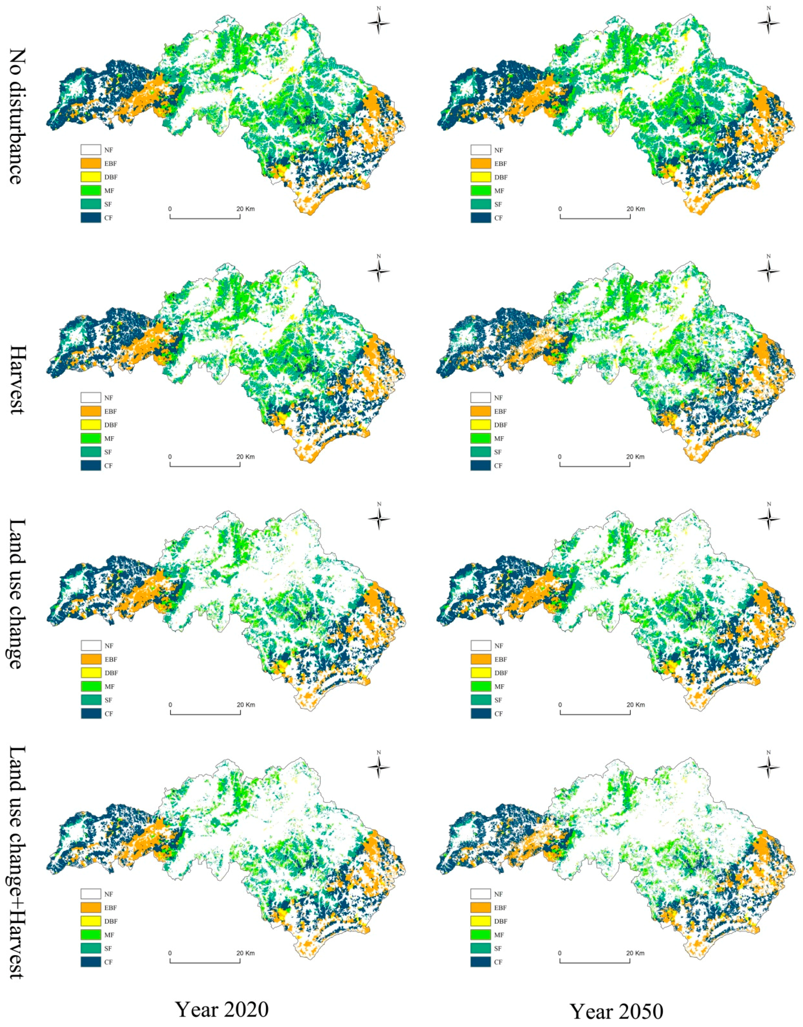
Four different scenarios were used in the LANDIS-II modeling to compare differences in the forest landscape in response to different disturbances. The spatial distribution of five forest types is shown in Figure 6. For the time dimension, there is little change in the forest landscape pattern for each scenario from 2020 to 2050. With the disturbances, the fragmentation of the forest landscape will increase, especially under the harvest and integrated scenarios. The results show that the change in the spatial pattern for EBF and SF will be more significant. In terms of forest landscape changes between the various scenarios, the results show a big difference in forest area. With only the harvest scenario, the forested area will reduce to different degrees for all the forest types. The largest area reduction will be the SF. Compared with the forest landscape without disturbance, the forest area of SF will decrease by 14,160 ha by 2050. Under the land use change scenario, the forest area shows a greater reduction than observed under the harvest scenario. The loss of forest mainly occurs in the central region where MF, SF, and DBF are distributed. Under the integrated scenario, the forest area will decrease the most with both harvest and land use change disturbances by the end of the simulation.
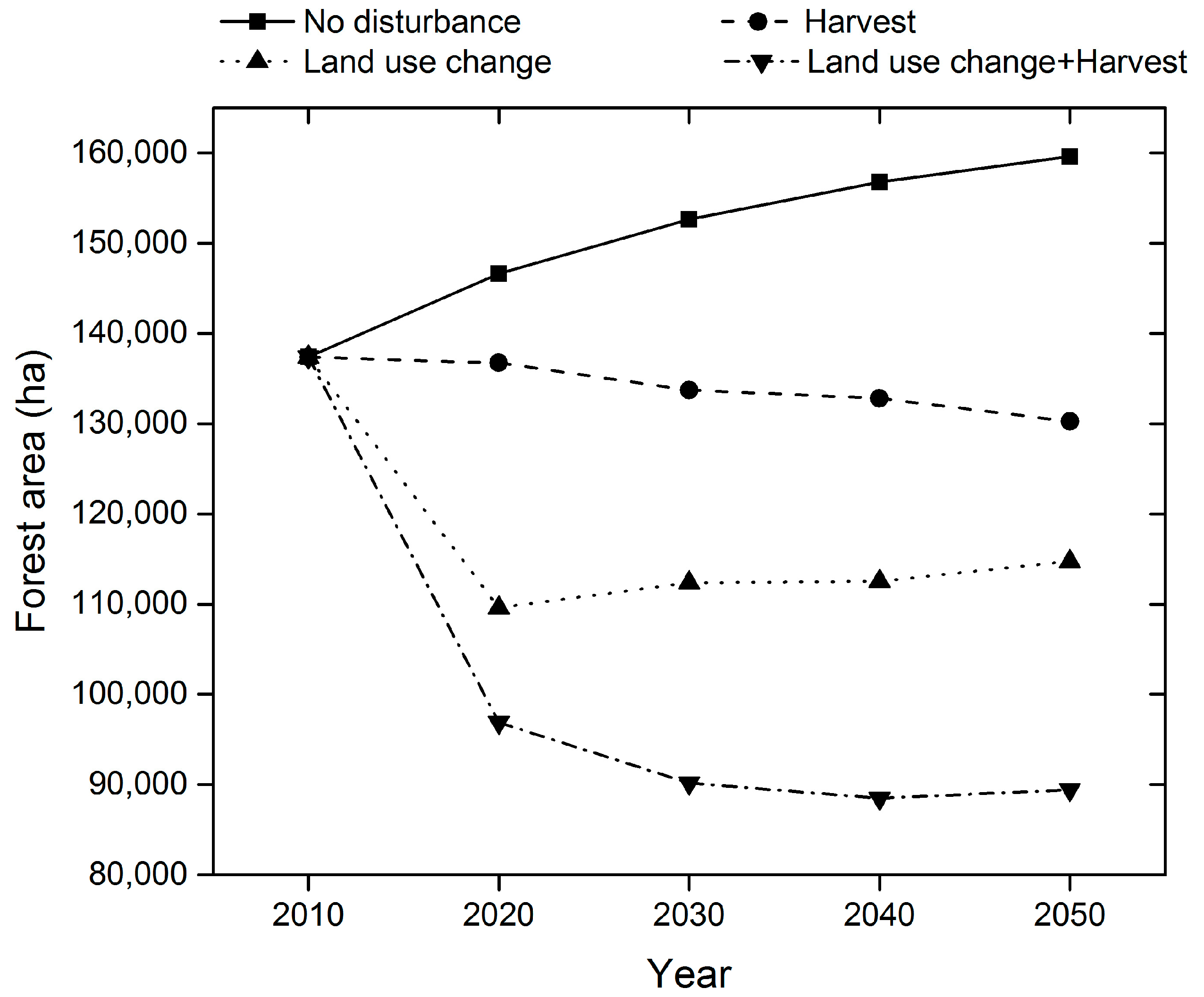
In terms of the variation in quantity, the simulated forest area will be used to describe the forest landscape change. The results under various disturbance scenarios are shown in Figure 7 and Table 2. The results show that differences begin to appear in 2020. Under the no disturbance scenario, the forest area will continuously increase from 2010 to 2050, increasing by 16.2% (22,245 ha). The DBF will increase the most, by 28.7% between 2010 and 2050. Under the harvest scenario, the forest area will decrease by 5.2% (7106 ha) to 2050 during the simulation. The biggest decline from 2010 to 2050 will be the SF, decreasing by 32.8%. The forest area shows the first severe decrease in 2020, and then progressively increases under land use change disturbance. Compared with 2010, the forest area will decrease by 16.5% (22,620 ha) in 2050. MF will be the forest type that is most heavily affected by land use change, decreasing by 33.6%. Additionally, the SF will also have a 32.6% decrease in forest area. Finally, under the integrated scenario, the forest area will drop even more dramatically, decreasing by 34.9% (47,943 ha) by 2050. The area for all forest types will be declining by 2050. The SF will decrease by 67.5%. The simulated results indicate that the forest landscape will be under pressure from land use change and harvest, which may result in the loss of forest area and changes in the landscape structure.
3.3. Relative Contributions of Land Use Change and Harvest
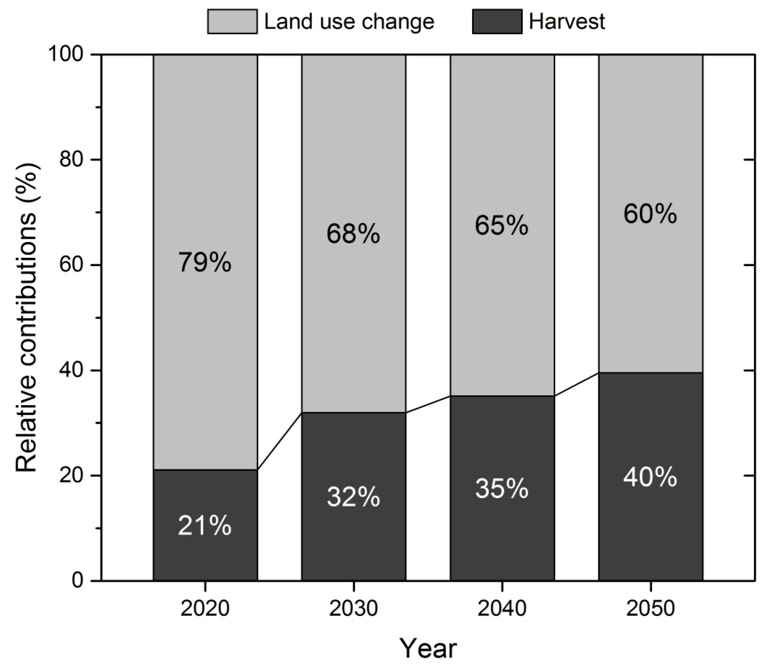
Four scenarios were carried out to quantitatively evaluate the relative contributions of forest conversion and harvest on the forest landscape change. The forest landscape remains undisturbed at the initial year of 2010. Therefore, the relative contributions are shown in Figure 8 for every time point from 2020 to 2050. The results show that the relative contributions of harvest will almost double from 21% to 40 % during the period from 2020 to 2050 (Figure 8). Conversely, the contributions of land use change to forest landscape change will reduce gradually, decreasing from 79% to 60%. However, the increasing relative contribution of harvest will not be consistent in each time period. Changes in the relative contributions of harvest in every decade from 2020 to 2050 will be 9%, 3%, and 5%.
4. Discussion
4.1. Uncertainties and Caveats
In this study, we used a coupled modeling framework to simulate the effects of land use change and harvest on forest landscape change. This coupling method between the models can help us to realize our objectives. However, there are still some uncertainties in our simulation. First, our study was based on some assumptions: (1) We integrated the CA-Markov model with the LANDIS-II model to generate a modeling framework, and we assumed that there was no interactive effect between these two models. That is, the land use change simulation and forest landscape simulation are independent. However, there may be a complex interaction between the different stakeholders that affects human decision-making, cognition, and behavior in the real world [49]; (2) We assumed that the forest landscape only changed under the land use change and harvest disturbances. However, other natural and anthropogenic disturbances, such as climate change, fire, and insect pests, may also affect the forest landscape change [50,51,52]; (3) In addition, we assumed that the climate, phenology, soil, terrain, and the transition probabilities matrix of the land use type in the future simulation are consistent with those in the contemporary condition. Although these assumptions may increase uncertainty in the simulation, they are necessary and reasonable for simplifying the simulation process. Second, the uncertainties may be derived from the models. The CA-Markov model can simulate the process of land cover change, but it is commonly criticized for its incapability of incorporating human decision-making [53]. This is because the model uses the stationarity of transition rules in different time steps and cannot account for the driving factors of land use change [20,54]. In addition, the accuracy of the land use change projection may be expected to decrease over time [31]. The current scenarios can be considered reliable for the simulation of land use in the near future (about 20 years). However, the different estimation errors for the further scenarios occurring over a period of 30–40 years can affect the results. The LANDIS-II model is a forest landscape stochastic model, which simulates forest landscape dynamics on a broad-scale with cohorts rather than for every stem [22]. The harvest events are also stochastically selected for implementation, which may add some randomness to the simulation result. Finally, the selection of the simulation periods also contributes to the uncertainties. Generally, the processes of land-use change are complex and drastic, and are greatly influenced by policy and the local government, especially in China. Therefore, the simulation of land use for a relatively long-term period is prone to uncertainty. In this study, the simulated period of 2010–2050 was selected based on some considerations. The land use datasets from Taihe County show that the spatial pattern of land use and cover has remained very similar in recent years. Town expansion has remained at a steady rate. Meanwhile, long-term successional development processes are required to identify changes in the forest landscape. By 2050, the simulation may reflect an overall change under the disturbances, especially under harvest. Therefore, the period of 2010–2050 was chosen due to the trade-off of the time effect between land use change and harvest. For the validation, quantitative validation of simulating results through comparing forest inventory data at large spatial and temporal scales is very difficult, especially for the predicted study. However, we still have confidence in our results. First, the LANDIS-II model has been previously applied in this area [23]. The validity of PnET models has also been verified [48]. Secondly, ecological input parameters are reliable, which are derived from forestry inventory data and an ecological station. Finally, the outputs of our simulation are reasonable, and in accordance with expert knowledge. Although there are some uncertainties in our studies, they do not prevent us from achieving our research objectives. In the future, we will improve our simulation as much as possible to overcome the deficiency and uncertainty of forest landscape simulation.
4.2. Implications of Quantitative Simulation for Future Management and Planning
Forest disturbances are ubiquitous worldwide, and their effects are demonstrated at different levels from species and communities to the forest ecosystem. Changes in the forest landscape are usually the result of complex natural and human disturbances, such as climate change, urbanization, harvest, and other land use demands [11,55]. As human activities increase, more influence has been exerted on the forest ecosystem. Land use change and harvest events are the two important disturbances which are usually followed by a more direct and instant impact on the forest landscape [56]. More specifically, land use pressures have a significant impact on forest characteristics, potentially causing a decline in the forest cover at a regional scale [3]. Timber cutting can change the forest landscape pattern more directly, especially in regions where plantations dominate [13,57]. With the development of the theory and technology of forest science, the simulation models and methods offer an efficient way to quantitatively simulate forest dynamic disturbances. An increasing number of forest simulation studies, from different parts of the world, reveal the importance of complex human disturbances in forest management [23,24,58]. In our study, the relative contribution of quantitative research was based on the land use model and forest landscape model coupling, and it was an attempt to resolve the complex disturbance process. We believe that the coupled modeling framework and method can combine the land system with a forest ecosystem, and may provide a solution for the other cases of forest disturbance simulation around the world. At the same time, the coupling simulation method can also make a contribution to the knowledge of forest disturbance research.
As important disturbances, land use change and harvest are both dominated by human activities, but differences also exist between them. The effect of land use change on a forest is usually associated with the conversion of land types, and the forestland is mainly transformed into build-up land, arable land, and orchards. In particular, forested area conversion to built-up land, driven by demand, is usually an irreversible process. Our simulation shows that the forest conversion zones caused by land use change mainly concentrate in the densely inhabited central district. Due to the intensive human activities and demand for economic benefits and housing, most central forestland will be invaded by urban construction land, orchards, and other land types. This effect of land use on forest was also observed in the study of Thompson et al. [14] in Massachusetts, USA. They used the probability of conversion to simulate the forest conversion zones by considering the relationship between forestland and factors, such as the population density, house density, and road density. Then, they found that the factor of population density contributes the most to the probability of forestland conversion. Harvest, compared to land use change, is a forest management activity for the purpose of timber production. The effect of harvest on forests manifests as the change of the forest’s internal structure. The simulation results show that harvest will make the forest landscape more fragmented for all kinds of forest types, especially for coniferous forest. This is because these coniferous species are the main kind of plantation in Taihe County and they have been defined prior to harvest simulation. Although the fragmentation will be intensified by harvest events, it will also reduce the density of mature, reproducing individuals that can disperse seeds and contribute to range expansion [59], which may benefit regional forest development. In addition, we found that the negative effect of land use change is waning and is beginning to have a positive effect on forest landscape change under the integrated scenario. The main reason for this is the irreversibility of the forest conversion caused by the land use change in our simulation, and these land use change effects reflect the initial stage of the simulation. However, the intensity of harvest remained unchanged during the simulation, so the effect of harvest is increasing. The result of the quantitative simulation can help understand the driving force of forest cover dynamics and is crucial for forest management and land use planning.
Forest disturbance has both positive and negative effects on forest landscape change. The disturbance is not only the main driving force for forest loss, but it is also an important means of forest management and regulation. The positive effects of human disturbance can help build a favorable forest site environment for forest natural regeneration and make a great contribution to the forest development [60]. Based on the representative forest type, economic development model, and forest management manner, we believe that our quantitative simulation results have certain universality, which can help develop more effective strategies for forest and land use management. Specifically, town development scale and speed should be properly controlled and scientifically planned to avoid an excessive expansion of the town in the future. The forested area that may be converted into built-up land should be strictly limited, ensuring a stable forested area ratio and the balanced proportions of different forest types in our study. For the regions where plantation dominated, the wood production is closely linked with the local economy. It is a big problem to weigh the relationship between economic development, wood production, and ecological protection. Additionally, it is also a challenge for policy makers to make timely adjustments to land use plans within a changing environment. In addition, disturbances will also have an effect on forest ecological succession, functional processes, and ecosystem services [58]. The effect of complex interference processes on forests will be the focus of future quantitative research, and it will better serve regional forests and sustainable land use development.
5. Conclusions
This study simulated and quantified the forest landscape dynamic under the disturbances of land use change and harvest from 2010 to 2050. The results show that land use change mainly occurs in the center of our study area, and the harvest events are in the coniferous forest area. The forest landscape will be under pressure from land use change and harvest, which may result in the significant loss of forest area. The quantitative results show that the forest area under harvest, land use change, and integrated scenarios will be reduced by 5.2%, 16.5%, and 34.9%, respectively. The results of the relative contribution indicate that the effects of land use change on the loss of forest cover will gradually weaken, but the effects of harvest will intensify accordingly. The quantitative simulation results may benefit the integration of regional forest management and land use policy decisions, enhance our understanding of the driving forces of forest landscape change, and contribute to achieving a trade-off between economic development and ecological environment construction.
Acknowledgments
This research was supported by National Key Basic Research Program of China (973 Program) (2015CB452702), National Natural Science Foundation of China (41571098, 41530749 & 41371196), Key Programs of the Chinese Academy of Sciences (ZDRW-ZS-2016-6-4) and A Major Consulting Project of Strategic Development Institute, Chinese Academy of Sciences (Y02015003).
Author Contributions
Zhuo Wu and Erfu Dai had the original idea for the study. Zhuo Wu was responsible for data modeling, analysis, and writing of the manuscript. Quansheng Ge and Erfu Dai reviewed the manuscript. Many thanks go to the anonymous reviewers for their valuable comments on this manuscript.
Conflicts of Interest
The authors declare no conflict of interest.
Abbreviations
The following abbreviations are used in this manuscript.
| CA | Cellular Automata |
| EBF | Evergreen Broad-leaved Forests |
| DBF | Deciduous Broad-leaved Forests |
| MF | Masson pine Forests |
| SF | Slash pine Forests |
| CF | Chinese fir Forests |
| OF | Other Forests |
| NF | Non-Forestland |
| QYZ station | Qian Yan Zhou ecological station |
| PAR | Photosynthetically Active Radiation |
| MCE | Multi-Criteria Evaluation |
| SEP | Species Establishment Probability |
| ANPP | Aboveground Net Primary Production |
| WHC | Water Holding Capacity |
| WUE | Water Use Efficiency |
| FL | Forestland |
| GL | Grass Land |
| WB | Water Body |
| BL | Built-up Land |
| UL | Unused Land |
| AL | Arable Land |
References
- Food and Agriculture Organization of the United Nations. Global Forest Resource Assessment 2010; FAO: Rome, Italy, 2010. [Google Scholar]
- Ninan, K.N.; Inoue, M. Valuing forest ecosystem services: What we know and what we don’t. Ecol. Econ. 2013, 93, 137–149. [Google Scholar] [CrossRef]
- Drummond, M.A.; Loveland, T.R. Land-use pressure and a transition to forest-cover loss in the eastern united states. Bioscience 2010, 60, 286–298. [Google Scholar] [CrossRef]
- Hansen, M.C.; Potapov, P.V.; Moore, R.; Hancher, M.; Turubanova, S.A.; Tyukavina, A.; Thau, D.; Stehman, S.V.; Goetz, S.J.; Loveland, T.R.; et al. High-resolution gloabl maps of 21st-century forest cover change. Science 2013, 342, 850–853. [Google Scholar] [CrossRef] [PubMed]
- Hansen, A.J.; Neilson, R.P.; Dale, V.H.; Flather, C.H.; Iverson, L.R.; Currie, D.J.; Shafer, S.; Cook, R.; Bartlein, P.J. Global change in forests: Responses of species, communities, and biomes. Bioscience 2001, 51, 775–779. [Google Scholar] [CrossRef]
- Newton, A.C.; Echeverría, C.; Cantarello, E.; Bolados, G. Projecting impacts of human disturbances to inform conservation planning and management in a dryland forest landscape. Biol. Conserv. 2011, 144, 1949–1960. [Google Scholar] [CrossRef]
- Gustafson, E.J.; Shvidenko, A.Z.; Sturtevant, B.R.; Scheller, R.M. Predicting global change effects on forest biomass and composition in south-central siberia. Ecol. Appl. 2010, 20, 700–715. [Google Scholar] [CrossRef] [PubMed]
- Barlow, J.; Lennox, G.D.; Ferreira, J.; Berenguer, E.; Lees, A.C.; Mac Nally, R.; Thomson, J.R.; Ferraz, S.F.; Louzada, J.; Oliveira, V.H.; et al. Anthropogenic disturbance in tropical forests can double biodiversity loss from harvest. Nature 2016, 535, 144–147. [Google Scholar] [CrossRef] [PubMed]
- Jõgiste, K.; Jonsson, B.G.; Kuuluvainen, T.; Gauthier, S.; Moser, W.K. Forest landscape mosaics: Disturbance, restoration, and management at times of global change. Can. J. For. Res. 2015, 45, v–vi. [Google Scholar] [CrossRef]
- Yeboah, D.; Chen, H.Y.H. Diversity–disturbance relationship in forest landscapes. Landsc. Ecol. 2015, 31, 981–987. [Google Scholar] [CrossRef]
- Rudel, T.K.; Coomes, O.T.; Moran, E.; Achard, F.; Angelsen, A.; Xu, J.; Lambin, E. Forest transitions: Towards a global understanding of land use change. Glob. Environ. Chang. 2005, 15, 23–31. [Google Scholar] [CrossRef]
- Steenberg, J.W.N.; Duinker, P.N.; Bush, P.G. Modelling the effects of climate change and timber harvest on the forests of central Nova Scotia, Canada. Ann. For. Sci. 2012, 70, 61–73. [Google Scholar] [CrossRef]
- Scheller, R.M.; Mladenoff, D.J. A spatially interactive simulation of climate change, harvesting, wind, and tree species migration and projected changes to forest composition and biomass in northern Wisconsin, USA. Glob. Chang. Biol. 2005, 11, 307–321. [Google Scholar] [CrossRef]
- Thompson, J.R.; Foster, D.R.; Scheller, R.M.; Kittredge, D. The influence of land use and climate change on forest biomass and composition in Massachusetts, USA. Ecol. Appl. 2011, 21, 2425–2444. [Google Scholar] [CrossRef] [PubMed]
- Abood, S.A.; Lee, J.S.H.; Burivalova, Z.; Garcia-Ulloa, J.; Koh, L.P. Relative contributions of the Logging, Fiber, Oil Palm, and mining industries to forest loss in Indonesia. Conserv. Lett. 2015, 8, 58–67. [Google Scholar] [CrossRef]
- Fang, J.Y.; Guo, Z.D.; Hu, H.F.; Kato, T.; Muraoka, H.; Son, Y. Forest biomass carbon sinks in East Asia, with special reference to the relative contributions of forest expansion and forest growth. Glob. Chang. Biol. 2014, 20, 2019–2030. [Google Scholar] [CrossRef] [PubMed]
- Pallett, R.N.; Sale, G. The relative contributions of tree improvement and cultural practice toward productivity gains in Eucalyptus pulpwood stands. For. Ecol. Manag. 2004, 193, 33–43. [Google Scholar] [CrossRef]
- Dai, E.; Wu, Z.; Wang, X.; Fu, H.; Xi, W.; Pan, T. Progress and prospect of research on forest landscape model. J. Geogr. Sci. 2014, 25, 113–128. [Google Scholar] [CrossRef]
- Sang, L.; Zhang, C.; Yang, J.; Zhu, D.; Yun, W. Simulation of land use spatial pattern of towns and villages based on CA-Markov model. Math. Comput. Model. 2011, 54, 938–943. [Google Scholar] [CrossRef]
- Adhikari, S.; Southworth, J. Simulating forest cover changes of Bannerghatta national park based on a CA-Markov model: A remote sensing approach. Remote Sens. 2012, 4, 3215–3243. [Google Scholar] [CrossRef]
- Yang, X.; Zheng, X.; Chen, R. A land use change model: Integrating landscape pattern indexes and Markov-CA. Ecol. Model. 2014, 283, 1–7. [Google Scholar] [CrossRef]
- Scheller, R.M.; Domingo, J.B.; Sturtevant, B.R.; Williams, J.S.; Rudy, A.; Gustafson, E.J.; Mladenoff, D.J. Design, development, and application of LANDIS-II, a spatial landscape simulation model with flexible temporal and spatial resolution. Ecol. Model. 2007, 201, 409–419. [Google Scholar] [CrossRef]
- Dai, E.; Wu, Z.; Ge, Q.; Xi, W.; Wang, X. Predicting the responses of forest distribution and aboveground biomass to climate change under RCPs scenarios in southern China. Glob. Chang. Biol. 2016, 22, 3642–3661. [Google Scholar] [CrossRef] [PubMed]
- Gustafson, E.J.; Shvidenko, A.Z.; Scheller, R.M. Effectiveness of forest management strategies to mitigate effects of global change in south-central Siberia. Can. J. For. Res. 2011, 41, 1405–1421. [Google Scholar] [CrossRef]
- Liu, S.R.; Wu, S.R.; Wang, H. Managing planted forests for multiple uses under a changing environment in China. NZ J. For. Sci. 2014, 44, S3. [Google Scholar] [CrossRef]
- Wang, Y.; Li, Q.; Wang, H.; Wen, X.; Yang, F.; Ma, Z.; Liu, Y.; Sun, X.; Yu, G. Precipitation frequency controls interannual variation of soil respiration by affecting soil moisture in a subtropical forest plantation. Can. J. For. Res. 2011, 41, 1897–1906. [Google Scholar] [CrossRef]
- South Hilly Scientific Expedition by Chinese Academy of Sciences. Natural Resource and Agricultural Regionalization in Taihe County, Jiangxi Province; Energy Press: Beijing, China, 1982. [Google Scholar]
- Han, J.; Hayashi, Y.; Cao, X.; Imura, H. Application of an integrated system dynamics and cellular automata model for urban growth assessment: A case study of Shanghai, China. Landsc. Urban Plan. 2009, 91, 133–141. [Google Scholar] [CrossRef]
- Clark Labs. IDRISI Geographic Information Systems and Remote Sensing Software; Clark Labs: Worcester, MA, USA, 2006. [Google Scholar]
- Eastman, J.R.; Jiang, H.; Toledano, J. Multi-criteria and multi-objective decision making for land allocation using GIS. In Multicriteria Analysis for Land-Use Management; Beinat, E., Nijkamp, P., Eds.; Springer: Dordrecht, The Netherlands, 1998; pp. 227–251. [Google Scholar]
- Pontius, R.G.J.; Huffaker, D.; Denman, K. Useful techniques of validation for spatially explicit land-change models. Ecol. Model. 2004, 179, 445–461. [Google Scholar] [CrossRef]
- Viera, A.J.; Garrett, J.M. Understanding interobserver agreement: The kappa statistic. Fam. Med. 2005, 37, 360–363. [Google Scholar] [PubMed]
- Scheller, R.M.; Mladenoff, D.J. A forest growth and biomass module for a landscape simulation model, LANDIS: Design, validation, and application. Ecol. Model. 2004, 180, 211–229. [Google Scholar] [CrossRef]
- Mladenoff, D.J.; Host, G.E.; Boeder, J.; Crow, T.R. LANDIS: A spatial model of forest landscapedisturbance, succession and management. In GIS and Environmental Modeling: Progress and Research Issues; Goodchild, M.F., Steyaert, L.T., Parks, B.O., Eds.; GIS World Books: Fort Collins, CO, USA, 1996. [Google Scholar]
- Mladenoff, D.J.; He, H. Design and behavior of LANDIS, an object-oriented model of forest landscape disturbance and succession. In Spatial Modeling Offorest Landscape Change: Approaches and Applications; Mladenoff, D.J., Baker, W.L., Eds.; Cambridge University Press: Cambridge, UK, 1999. [Google Scholar]
- De Bruijn, A.; Gustafson, E.J.; Sturtevant, B.R.; Foster, J.R.; Miranda, B.R.; Lichti, N.I.; Jacobs, D.F. Toward more robust projections of forest landscape dynamics under novel environmental conditions: Embedding PnET within LANDIS-II. Ecol. Model. 2014, 287, 44–57. [Google Scholar] [CrossRef]
- Xu, C.; Gertner, G.Z.; Scheller, R.M. Importance of colonization and competition in forest landscape response to global climatic change. Clim. Chang. 2011, 110, 53–83. [Google Scholar] [CrossRef]
- Chen, X.; Li, W.; Pan, Q.; Yang, M. Studies on spacial distribution and the spread distance of pollen in Chinese fir seed orchards. J. Beijing For. Univ. 1996, 18, 24–30. [Google Scholar]
- Editorial Committee of Forest of China. Forest of China; China Forestry Publishing House: Beijing, China, 2000; Volumes 2–3. [Google Scholar]
- Yu, Q.; Wang, S.; Shi, H.; Huang, K.; Zhou, L. An evaluation of spaceborne imaging spectrometry for estimation of forest canopy nitrogen concentration in a subtropical conifer plantation of southern China. J. Resour. Ecol. 2014, 5, 1–10. [Google Scholar]
- Wu, Z.L. Chinese Fir; China Forestry Publish House: Beijing, China, 1984. [Google Scholar]
- He, K.; Liu, R.L. Encyclopedia of Chinese Agriculture: Forestry Volume; China Agriculture Press: Beijing, China, 1989. [Google Scholar]
- Sheng, W.; Ren, S.; Yu, G.; Fang, H.; Jiang, C.; Zhang, M. Patterns and driving factors of WUE and NUE in natural forest ecosystems along the north-south transect of eastern China. J. Geogr. Sci. 2011, 21, 651–665. [Google Scholar] [CrossRef]
- Aber, J.D.; Federer, C.A. A generalized, lumped-parameter model of photosynthesis, evapotranspiration and net primary production in temperate and boreal forest ecosystems. Oecologia 1992, 92, 463–474. [Google Scholar] [CrossRef] [PubMed]
- Aber, J.D.; Ollinger, S.V.; Federer, C.A.; Reich, P.B.; Goulden, M.L.; Kicklighter, D.W.; Melillo, J.M.; Lathrop R.G., Jr. Predicting the effects of climate change on water yield and forest production in the northeastern United States. Clim. Res. 1995, 5, 207–222. [Google Scholar] [CrossRef]
- Aber, J.D.; Driscoll, C.T. Effects of land use, climate variation, and N deposition on N cycling and C storage in northern hardwood forests. Glob. Biogeochem. Cycles 1997, 11, 639–648. [Google Scholar] [CrossRef]
- Ollinger, S.V.; Aber, J.D.; Reich, P.B.; Freuder, R.J. Interactive effects of nitrogen deposition, tropospheric ozone, elevated CO2 and land use history on the carbon dynamics of northern hardwood forests. Glob. Chang. Biol. 2002, 8, 545–562. [Google Scholar] [CrossRef]
- Liu, Y.P.; Yu, D.Y.; Xun, B.; Sun, Y.; Hao, R.F. The potential effects of climate change on the distribution and productivity of Cunninghamia lanceolata in China. Environ. Monit. Assess. 2014, 186, 135–149. [Google Scholar] [CrossRef] [PubMed]
- Robinson, D.T.; Sun, S.; Hutchins, M.; Riolo, R.L.; Brown, D.G.; Parker, D.C.; Filatova, T.; Currie, W.S.; Kiger, S. Effects of land markets and land management on ecosystem function: A framework for modelling exurban land-change. Environ. Model. Softw. 2013, 45, 129–140. [Google Scholar] [CrossRef]
- Berland, A.; Shuman, B.; Manson, S.M. Simulated importance of dispersal, disturbance, and landscape history in long-term ecosystem change in the big woods of Minnesota. Ecosystems 2011, 14, 398–414. [Google Scholar] [CrossRef]
- He, H.; Mladenoff, D.J. Spatially explicit and stochastic simulation of forest landscape fire disturbance and succession. Ecology 1999, 80, 81–99. [Google Scholar] [CrossRef]
- Leroux, S.J.; Rayfield, B.; Rouget, M. Methods and tools for addressing natural disturbance dynamics in conservation planning for wilderness areas. Divers. Distrib. 2014, 20, 258–271. [Google Scholar] [CrossRef]
- Briassoulis, H. Analysis of Land Use Change: Theoretical and Modelling Approaches; Regional Research Institute, West Virginia University: Morgantown, WV, USA, 2000. [Google Scholar]
- Tattoni, C.; Ciolli, M.; Ferretti, F. The fate of priority areas for conservation in protected areas: A fine-scale Markov chain approach. Environ. Manag. 2011, 47, 263–278. [Google Scholar] [CrossRef] [PubMed]
- Gustafson, E.J.; Crow, T.R. Simulating the effects of alternative forest management strategies on landscape strcuture. J. Environ. Manag. 1996, 46, 77–94. [Google Scholar] [CrossRef]
- Wu, Z.; Dai, E.; Ge, Q.; Xi, W.; Wang, X. Modelling the integrated effects of land use and climate change scenarios on forest ecosystem aboveground biomass, a case study in Taihe County of China. J. Geogr. Sci. 2017, 27, 205–222. [Google Scholar] [CrossRef]
- Gustafson, E.J.; Shifley, S.R.; Mladenoff, D.J.; Nimerfro, K.K.; He, H. Spatial simulation of forest succession and timber harvesting using LANDIS. Can. J. For. Res. 2000, 30, 32–43. [Google Scholar] [CrossRef]
- Oliveira, P.J.C.; Asner, G.P.; Knapp, D.E.; Almeyda, A.; Galván-Gildemeister, R.; Keene, S.; Raybin, R.F.; Smith, R.C. Land-ues allocation protects the Peruvian Amazon. Science 2007, 317, 1233–1236. [Google Scholar] [CrossRef] [PubMed]
- Scheller, R.M.; Mladenoff, D.J. Simulated effects of climate change, fragementation, and inter-specific competition on tree species migration in northern Wisconsin, USA. Clim. Res. 2008, 36, 191–202. [Google Scholar] [CrossRef]
- Hong, S.K.; Nakagoshi, N.; Kamada, M. Human impacts on pine-dominated vegetation in rural landscapes in Korea and western Japan. Plant Ecol. 1995, 116, 161–172. [Google Scholar] [CrossRef]
Figure 1.
Location and forest type of the study area. EBF: evergreen broad-leaved forests; DBF: deciduous broad-leaved forests; MF: masson pine forests; SF: slash pine forests; CF: Chinese fir forests; OF: other forests; NF: non-forest land; QYZ station: Qianyanzhou ecological station.
Figure 1.
Location and forest type of the study area. EBF: evergreen broad-leaved forests; DBF: deciduous broad-leaved forests; MF: masson pine forests; SF: slash pine forests; CF: Chinese fir forests; OF: other forests; NF: non-forest land; QYZ station: Qianyanzhou ecological station.

Figure 2.
Framework for simulating the effects of land use change and harvest on forest landscapes.

Figure 3.
Land use maps (a) actual land use in 2010 and (b) simulated land use in 2010 using the CA-Markov model. FL: forest land; GL: grass land; WB: water body; BL: built-up land; UL: unused land; AL: arable land.
Figure 3.
Land use maps (a) actual land use in 2010 and (b) simulated land use in 2010 using the CA-Markov model. FL: forest land; GL: grass land; WB: water body; BL: built-up land; UL: unused land; AL: arable land.
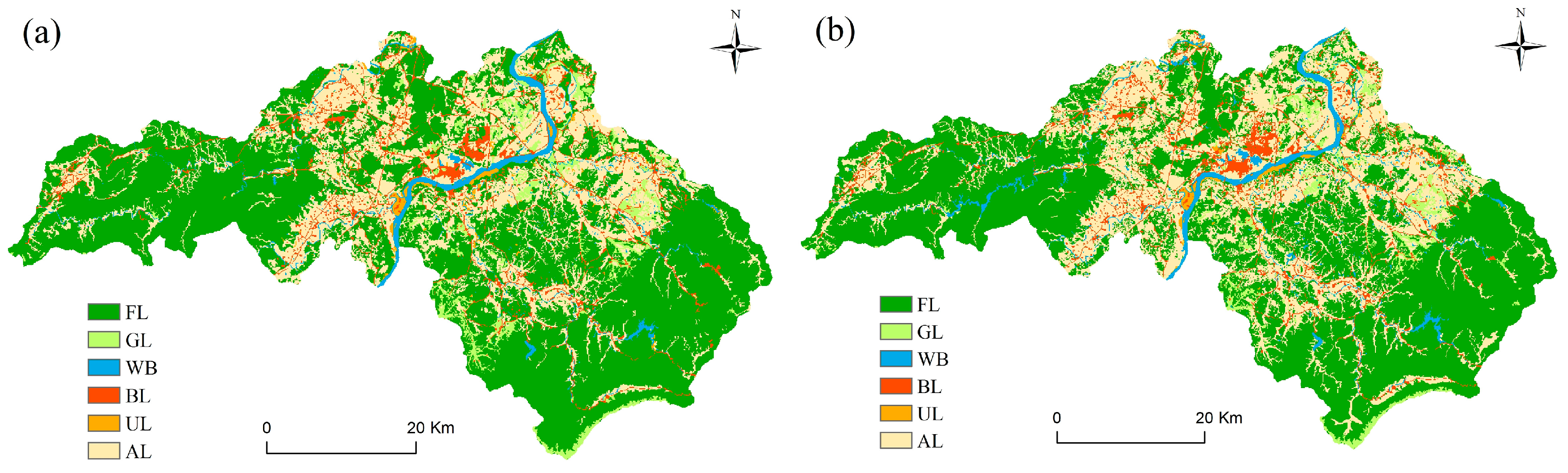
Figure 4.
Ecoregions of the study area.
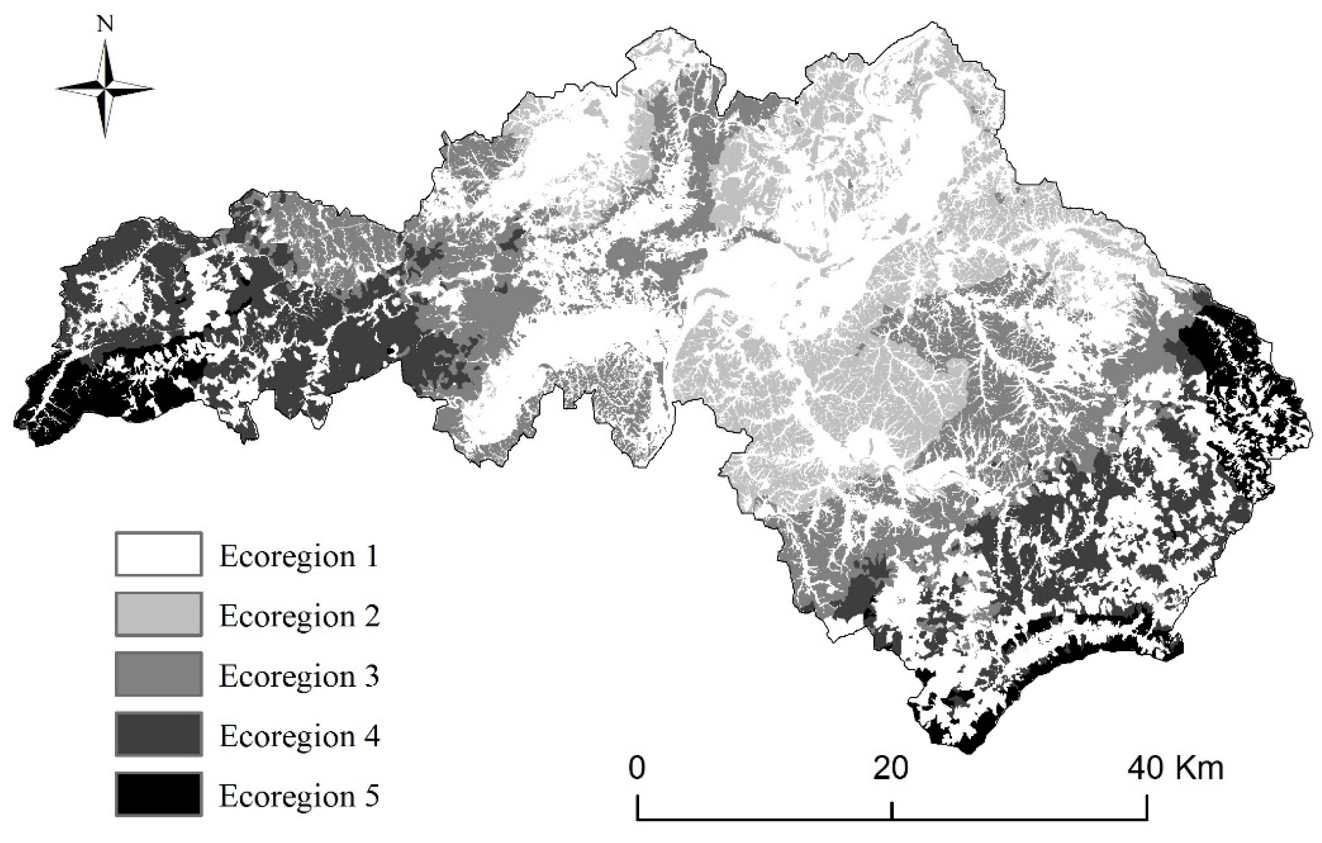
Figure 5.
Simulated land use maps generated using the CA-Markov model in 2020, 2030, 2040, and 2050.
Figure 5.
Simulated land use maps generated using the CA-Markov model in 2020, 2030, 2040, and 2050.
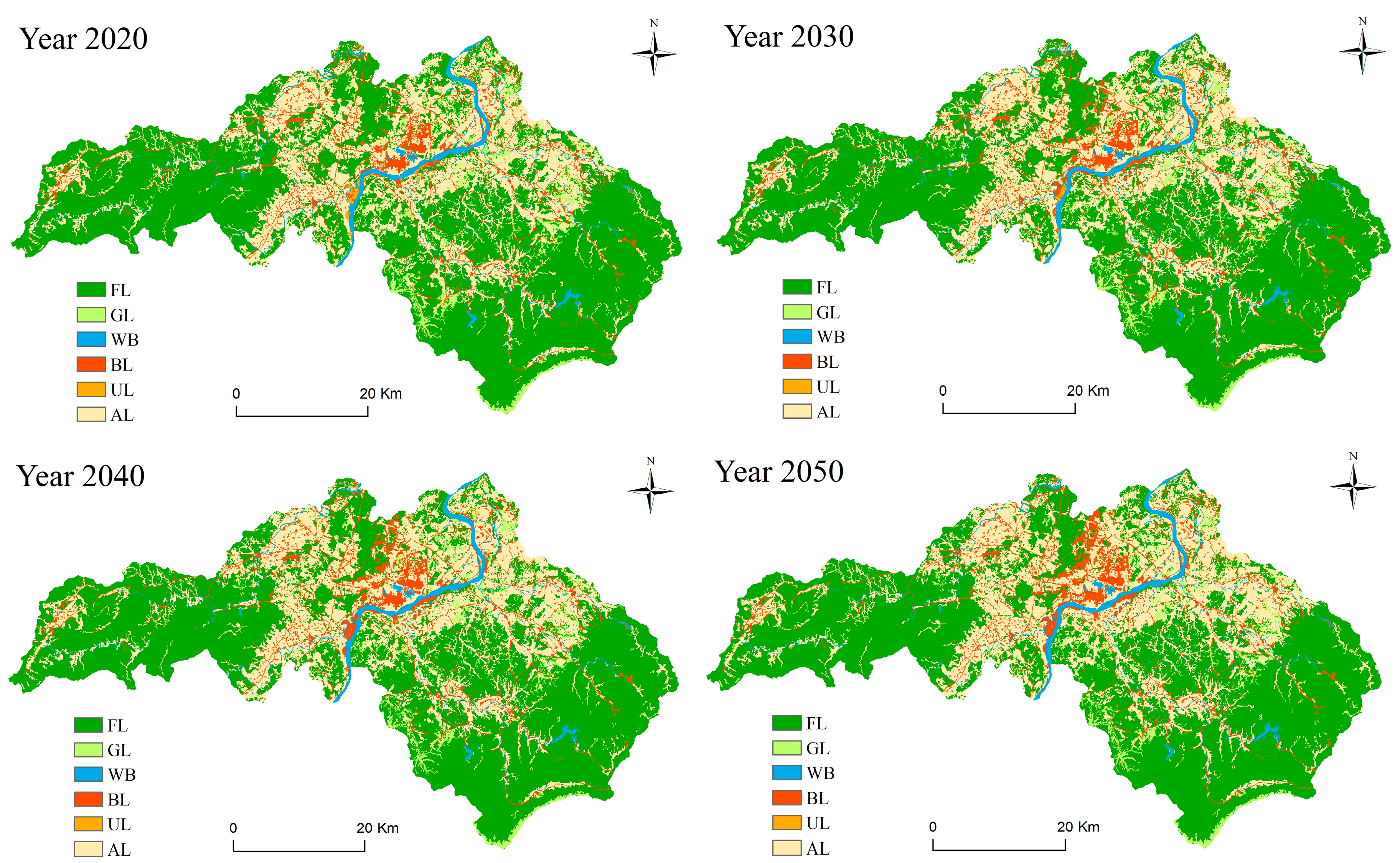
Figure 6.
Forest landscape pattern under no disturbance scenario, harvest scenario, land use change scenario, and integrated scenario (land use change + harvest) in 2020 and 2050.
Figure 6.
Forest landscape pattern under no disturbance scenario, harvest scenario, land use change scenario, and integrated scenario (land use change + harvest) in 2020 and 2050.

Figure 7.
Forest area variation under no the disturbance scenario, harvest scenario, land use change scenario, and integrated scenario (conversion + harvest) during 2010–2050.
Figure 7.
Forest area variation under no the disturbance scenario, harvest scenario, land use change scenario, and integrated scenario (conversion + harvest) during 2010–2050.

Figure 8.
Relative contributions of land use change and harvest to the forest landscape change.


Table 1.
Species life history attributes in Taihe County, Jiangxi Province, China.
| Species | Longevity (Year) | Sexual Maturity (Year) | Shade Tol. | Seed Dispersal Dist. | |
|---|---|---|---|---|---|
| Effective (m) | Maximum (m) | ||||
| Cunninghamia lanceolata | 200 | 10 | 1 | 200 | 500 |
| Cupressus funebris | 500 | 35 | 2 | 70 | 200 |
| Pinus massoniana | 200 | 10 | 1 | 200 | 500 |
| Pinus elliottii | 200 | 10 | 1 | 200 | 500 |
| Schima superba | 300 | 20 | 5 | 20 | 200 |
| Cinnamomum camphora | 1000 | 15 | 4 | 50 | 120 |
| Phoebe zhennan | 1000 | 50 | 5 | 40 | 120 |
| Castanopsis eyrei | 200 | 20 | 5 | 50 | 120 |
| Castanopsis fargesii | 150 | 30 | 5 | 60 | 250 |
| Quercus fabri | 120 | 15 | 4 | 20 | 200 |
| Cyclobalanopsis gracilis | 200 | 7 | 4 | 20 | 50 |
| Liquidambar formosana | 130 | 8 | 3 | 100 | 375 |
| Betula luminifera | 100 | 15 | 2 | 150 | 400 |
| Alnus cremastogyne | 125 | 5 | 3 | 15 | 60 |
| Alniphyllum fortunei | 120 | 15 | 2 | 250 | 500 |
| Sassafras tzumu | 120 | 20 | 3 | 50 | 150 |
| Melia azedarach | 80 | 5 | 2 | 200 | 400 |
| Populus deltoides | 90 | 10 | 2 | 150 | 500 |
Notes: Shade Tol. stands for the species’ tolerance to shade. The value is an integer between 1 and 5, where 1 represents the least tolerance and 5 represents the most tolerance. Seed Dispersal Dist. represents the species’ effective or maximum distance for dispersing seeds.
Table 2.
Variation in area for different forest type under different scenarios between 2010 and 2050.
Table 2.
Variation in area for different forest type under different scenarios between 2010 and 2050.
| Type | Initial | No Disturbance | Harvest | Land Use Change | Land Use Change + Harvest | ||||
|---|---|---|---|---|---|---|---|---|---|
| 2010 | 2050 | 2050 | 2050 | 2050 | |||||
| Area (ha) | Area (ha) | Rate (%) | Area (ha) | Rate (%) | Area (ha) | Rate (%) | Area (ha) | Rate (%) | |
| EBF | 23,105 | 26,645 | 15.3 | 22,796 | −1.3 | 23,813 | 3.1 | 19,459 | −15.8 |
| DBF | 2877 | 3704 | 28.7 | 3821 | 32.8 | 2118 | −26.4 | 2122 | −26.2 |
| MF | 27,282 | 32,700 | 19.9 | 29,440 | 7.9 | 18,123 | −33.6 | 15,602 | −42.8 |
| SF | 43,170 | 49,887 | 15.6 | 29,010 | −32.8 | 29,096 | −32.6 | 14,027 | −67.5 |
| CF | 40,943 | 46,686 | 14.0 | 45,204 | 10.4 | 41,607 | 1.6 | 38,224 | −6.6 |
| Total | 137,377 | 159,622 | 16.2 | 130,271 | −5.2 | 114,757 | −16.5 | 89,434 | −34.9 |
Notes: Land use change + harvest means integrated scenario under both land use change and harvest. Rate means the change rates of forest area between 2010 and 2050. Total means the simulated holistic forest landscape.
© 2017 by the authors. Licensee MDPI, Basel, Switzerland. This article is an open access article distributed under the terms and conditions of the Creative Commons Attribution (CC BY) license (http://creativecommons.org/licenses/by/4.0/).
Share and Cite
MDPI and ACS Style
Wu, Z.; Ge, Q.; Dai, E. Modeling the Relative Contributions of Land Use Change and Harvest to Forest Landscape Change in the Taihe County, China. Sustainability 2017, 9, 708. https://doi.org/10.3390/su9050708
AMA Style
Wu Z, Ge Q, Dai E. Modeling the Relative Contributions of Land Use Change and Harvest to Forest Landscape Change in the Taihe County, China. Sustainability. 2017; 9(5):708. https://doi.org/10.3390/su9050708
Chicago/Turabian StyleWu, Zhuo, Quansheng Ge, and Erfu Dai. 2017. "Modeling the Relative Contributions of Land Use Change and Harvest to Forest Landscape Change in the Taihe County, China" Sustainability 9, no. 5: 708. https://doi.org/10.3390/su9050708
Note that from the first issue of 2016, this journal uses article numbers instead of page numbers. See further details here.