
Establishment of the Sustainable Ecosystem for the Regional Shipping Industry Based on System Dynamics

1
School of Navigation, Wuhan University of Technology, Wuhan 430070, Hubei, China
2
Hubei Key Laboratory of Inland Shipping Technology, Wuhan 430063, Hubei, China
3
National Engineering Research Center for Water Transport Safety, Wuhan 430070, Hubei, China
*
Author to whom correspondence should be addressed.
Sustainability 2017, 9(5), 742; https://doi.org/10.3390/su9050742
Submission received: 17 December 2016
/
Revised: 26 April 2017
/
Accepted: 27 April 2017
/
Published: 4 May 2017
(This article belongs to the Special Issue Sustainable Ecosystems and Society in the Context of Big and New Data)
Abstract
:The rapid development of the shipping industry has brought great economic benefits but at a great environmental cost; exhaust emissions originating from ships are increasing, causing serious atmospheric pollution. Hence, the mitigation of ship exhaust emissions and the establishment of the sustainable ecosystem have become urgent tasks, which will require complicated and comprehensive systematic approaches to solve. We address this problem by establishing a System Dynamics (SD) model to help mitigate regional ship exhaust emissions without restricting economic growth and promote the development of the sustainable ecosystem. Factors correlated with ship exhaust emissions are identified, and a causal loop diagram is drawn to describe the complicated interrelations among the correlated factors. Then, a stock-and-flow diagram is designed and variable equations and parameter values are determined to quantitatively describe the dynamic relations among different elements. After verifying the effectiveness of the model, different scenarios for the sustainable development in the study area were set by changing the values of the controlling variables. The variation trends of the exhaust emissions and economic benefits for Qingdao port under different scenarios were predicted for the years 2015–2025. By comparing the simulation results, the effects of different sustainable development measures were analyzed, providing a reference for the promotion of the harmonious development of the regional environment and economy.
1. Introduction
Green House Gas (GHG) emissions are the principal factors affecting the global climate change. In recent years, with ships becoming larger and more numerous, the amount of GHG emissions originating from ships have been increasing rapidly. According to the Third IMO GHG Study [1], the total mass of CO2 emissions from the shipping industry in 2012 was 7.96 hundreds of millions, accounting for 2.2% of the global amount in the same year. Therefore, it has been becoming an ever more urgent task to take measures to control ship exhaust emissions. If un-controlled, GHG emissions from the shipping industry by 2050 are expected to increase 0.5 to 2.5 times over that in 2012.
Emission mitigation measures can be researched based on the calculation of ship exhaust emissions and the establishment of regional emission inventories. At present, more and more countries and regions have put forward detailed measures to control ship exhaust emissions, such as speed reduction [2,3], improving the energy consumption structure [4], using alternative energy [5], using shore electricity during berthing [6], and applying exhaust after-treatment technology [7]. While mitigation of regional ship exhaust emissions is not a simple task, it will require complicated and comprehensive systematic approaches to solve. Previous researches have focused mostly on the calculation of exhaust emissions and the establishment of regional emission inventories, rather than the establishment and analysis of the entire sustainable ecosystem. We address this problem by establishing a System Dynamics model to help mitigate regional ship exhaust emissions without restricting the economic growth and promote the development of the sustainable ecosystem, filling a gap in this research field.
System Dynamics (SD) is a methodology to analyze the information feedback among various elements, then recognize and solve the systematic problems [8,9,10]. It uses the computer software to make simulations to reflect the dynamic causal relationships and intrinsic mechanisms within the complicated system, which is high-order, nonlinear and multi-feedback. The main elements of the SD structure include flow, level, rate and auxiliary variables [11]. SD is aimed to realize the combination of qualitative and quantitative analysis to solve systematic problems more effectively. SD modeling includes the following five steps: The first step is to determine the main problems and research objective; the second step is to build the model framework, determine the feedback loops and casual loop diagram; the third step is to figure out the stock-flow diagram, and establish equations to describe the quantitative relations among each element; the fourth step is to verify the effectiveness of the model using SD software; and the final step is to set different scenarios, and compare the simulation results under each scenario to provide references for the decision-making process [12,13,14].
Many researchers have applied System Dynamics as a decision-making tool for the low-carbon development of regions and cities. For some examples, in China, the regional low-carbon model was established using SD and the effectiveness of the model is verified by comparing the simulation results to the historical data, then several scenarios were designed to make prediction of the future low-carbon development of China, based on which, countermeasures were proposed to reduce the CO2 emissions [15]. After that, the SD model of economy, energy and carbon emissions was constructed, considering different economy growth rate and different policy factor, then the energy consumption, carbon emissions and emission intensity of China from 2013 to 2020 are predicted, of which the results can provide references for the environmental development of China [14]. In Fujian city of China, the SD model for the low-carbon development was constructed and verification of the model is made based on the historical data from 2006 to 2011, then the low carbon economy development of Fujian city from 2012 to 2050 is simulated, and by comparing the simulation results, the optimal developing pattern was recognized [12]. In Beijing, China, the SD model, which consists of six sub-models of social economy, agriculture, industry, service, population and transportation, was constructed. Then the energy consumption and carbon emissions from 2005 to 2030 in Beijing were calculated, and it is discovered that the transformation of development pattern and control of the population increase can effectively reduce the energy consumption and carbon emissions [13]. In Ecuador, the SD model was built to study the influences of changing the energy matrix on the CO2 emissions. Simulation results show that using renewable energy and improving the productive sectoral structure can effectively reduce the CO2 emissions. The model proposed in this paper can be used as a policy-making tool because it is transferable to any other time period or region [16]. In Jakarta, Indonesia, the SD model was constructed to simulate the economy development and CO2 emissions under three different conditions, this research can provide suggestions for the balanced development of economy and environment [17]. We can see that System Dynamics can be well applied to research the regional development considering all kinds of different factors, such as carbon emission, energy consumption, economic development, policy making, etc. Taking the variable of carbon emission as the objective, qualitative and quantitative researches can be done on the complicated causal relationships and feedback mechanisms between the carbon emission and other related factors, based on which, prediction can be further made about the variation of carbon emissions under different conditions. Then, effective suggestions can be proposed for the better developing pattern of the region with the aim of sustainable development.
In addition, System Dynamics has a wide scope of application and can be used for the research of emission mitigation in various fields. For some examples, in transportation modeling, SD is applied to better understand the relationships within the transport system and between transport and the surrounding environment, then further the effectiveness of alternative transport-related policies [18]. In the electricity market of Latvian, the SD model is constructed and further verified using the historical data from 1995 to 2012. Then different policies are set to simulate the future development of the electricity market, the results show that increasing the ratio of natural gas in electricity supply can achieve CO2 emissions reduction greater than 30% by 2050 [19]. In the urban transport field, Beijing is taken as a case to construct the SD model to analyze the motorization trend and the CO2 emissions. It is found that the urban transport condition and CO2 emissions would become more serious with the growth of vehicle ownership and travel demand. Then emission values in 2020 were simulated under different scenarios to analyze the effectiveness of different measures [20]. In marine industry, an endogenous ship owner model was constructed to simulate the dynamics inherent in the sale of a vessel and subsequent financial implications, which can help the decision-making of ship owners [21]. In Chinese shipping industry, the SD model was constructed to simulate the effects of three emission reduction measures of technical, operational and market-based. The simulation results show that decreasing the ship speed and improving the energy consumption structure can effectively mitigate the emissions [22]. In the agricultural system in Latvia, the SD model was constructed based on the IPCC guidelines, then the GHG emissions under different scenarios are simulated. The simulation results have directive significance for the development of low-carbon economy, and by changing the values of some key parameters, this model can also be used as a policy-making tool for the development of other countries or districts [23]. In the iron and steel industry, the SD model was constructed based on energy, materials and process flow, to analyze the CO2 emission reduction technologies and energy use in iron and steel manufacturing processes. Six different CO2 reduction technologies were introduced to make comparison with the usual scenario to analyze the effects of different technologies [24]. Besides, System Dynamics can also be applied to many other fields, such as the cement industry [25], inter-city passenger transport industry [26], green transportation industry [27], electric power industry [28], animal farming industry [29], etc.
We can see that SD has wide application in many fields, in this paper, we put our focus on the application of SD methods to the sustainable development of the shipping industry, on which current researches are still not thorough enough. In this paper, SD methods are used to model the mitigation of regional exhaust emissions originating from ships, considering the complicated casual-and-effect relationships and feedback mechanisms among different elements. Then VENSIM (Ventana Simulation) simulations are made to predict the variation tendency of regional ship exhaust emissions and assess the economic benefits in the future, and can be taken as a reference for the development of the regional sustainable ecosystem.
The rest of this paper is as follows: Section 2 discusses in detail the measurement of the exhaust emissions for single ship and the establishment of regional emission inventories. Section 3 presents the model framework. Section 4 describes the study area and data sources. In Section 5, the simulation results are shown, and in Section 6, the key conclusions, limitations, and directions for future work are discussed.
2. Related Work
Most researches in this field have focused on the measurement and calculation of regional ship exhaust emissions rather than the mitigation of that. There are two widely-used methods to calculate ship exhaust emissions, that is, the “bottom-up” method and “top-down” method. The “top-down” method acquires the total fuel consumption data of ships and multiplies it by the average emission factor to get the total amount of ship exhaust emissions [30,31,32]. The emission factor represents the amount of emissions caused by per unit of fuel consumption. Conversely, the “bottom-up” method is based on ship activities. This method calculates the fuel consumption for different navigation statuses, then multiplies it by related emission factor to get the emissions amount under different navigation statuses respectively, summing them up to obtain the total amount of emissions for a single voyage [33,34]. In this instance, the value of the emission factor is determined according to the corresponding engine type and navigation status, therefore, is more precise than that in the “top-down” method.
On the basis of the emission calculation for single ship, a ship emission inventory for a region can be established; furthermore, the spatial and temporal distribution of emissions can be analyzed. Emission inventories for several Chinese cities and port areas have been established. For port of Dalian, the real-time data of Ocean Going Vessels (OGVs) such as speed, sailing time and geographical position have been acquired based on the Automatic Identification System (AIS), while an emission inventory for the whole year of 2012 was established using the “bottom-up” method. Based on this emission inventory, the spatial distribution of emissions was analyzed. The spatial distribution results show that the port area where ships moor and berth is the area with the most intensive emissions, that is, the amount of emissions per unit area in the port area is the largest compared with other areas [35]. It is worth noting that whether the “top-down” method or “bottom-up” method should be selected depends on the completeness of the acquired data. For example, to establish the emission inventory for Guangdong, emissions originating from passenger and cargo transportation ships were calculated using the “bottom-up” method based on the AIS data; while emissions originating from fishing ships were calculated using the “top-down” method based on fuel consumption as the AIS data were limited for fishing ships [36]. Besides, emission inventories for Tianjin port [37], Shanghai port [38], Pearl River Delta [39] and Shen zhen [40] have also been analyzed and established, all these emission inventories are established based on the “bottom-up” method combining the ship activity data acquired from AIS and other ship information databases
Abroad, emissions from transit vessels and passenger ships transporting on Turkish Straits were calculated using the “top-down” method [41]. For Hong Kong, the total exhaust emissions from OGVs are calculated using the “bottom-up” method based on the ship activity data. Results show that the proportion of emissions originating from container ships is the largest among all kinds of ships, and that of passenger ship is the second largest [42]. The total amount of exhaust emissions in the Baltic Sea during the whole year of 2007 is also calculated based on STEAM (Ship Traffic Estimation Assessment Model), which considered the influence of wave on fuel consumption and exhaust emissions [43]. In addition, the emission inventories for the largest port in Korea [44] and port of Taranto [45] are also established.
In this paper, we put our emphasis on the mitigation of regional ship exhaust emissions and the development of the sustainable ecosystem by applying the System Dynamics method.
3. Framework of the Sustainable Ecosystem
The primary objective of the proposed model is to realize the reduction of regional ship exhaust emissions without choking off the regional economic growth and promote the development of the sustainable ecosystem. The sustainable ecosystem suggested in this paper includes five sub-systems: the shipping, energy, environment, economy and policy components. The framework of the sustainable ecosystem for the regional shipping industry is shown as follows (Figure 1).
Among them, the shipping sub-system includes the ship speed, sailing time and port handling capacity, and ship speed is the main influence factor of fuel consumption. Energy sub-system represents the consumption of different kinds of energy, including fuel oil, low-sulfur oil and LNG. The improvement of the energy consumption structure can mitigate the ship emissions. Environment sub-system refers to the total amount of exhaust emissions originating from ships, which is closely related with the fuel consumption amount, and can be mitigated through the application of emission reduction measures. The economic sub-system includes economic incomes and costs. Economic incomes include the freight revenue, port income and the environmental benefit brought by emission reduction. Economic costs include the cost of consumed energy, construction cost of infrastructures, ship reconstruction cost and the pollution loss. Among these five sub-systems, the shipping sub-system is the core of the whole system, which has input and output relations with all the other four sub-systems.
3.1. Causal Loop Diagram and Main Feedback Loops
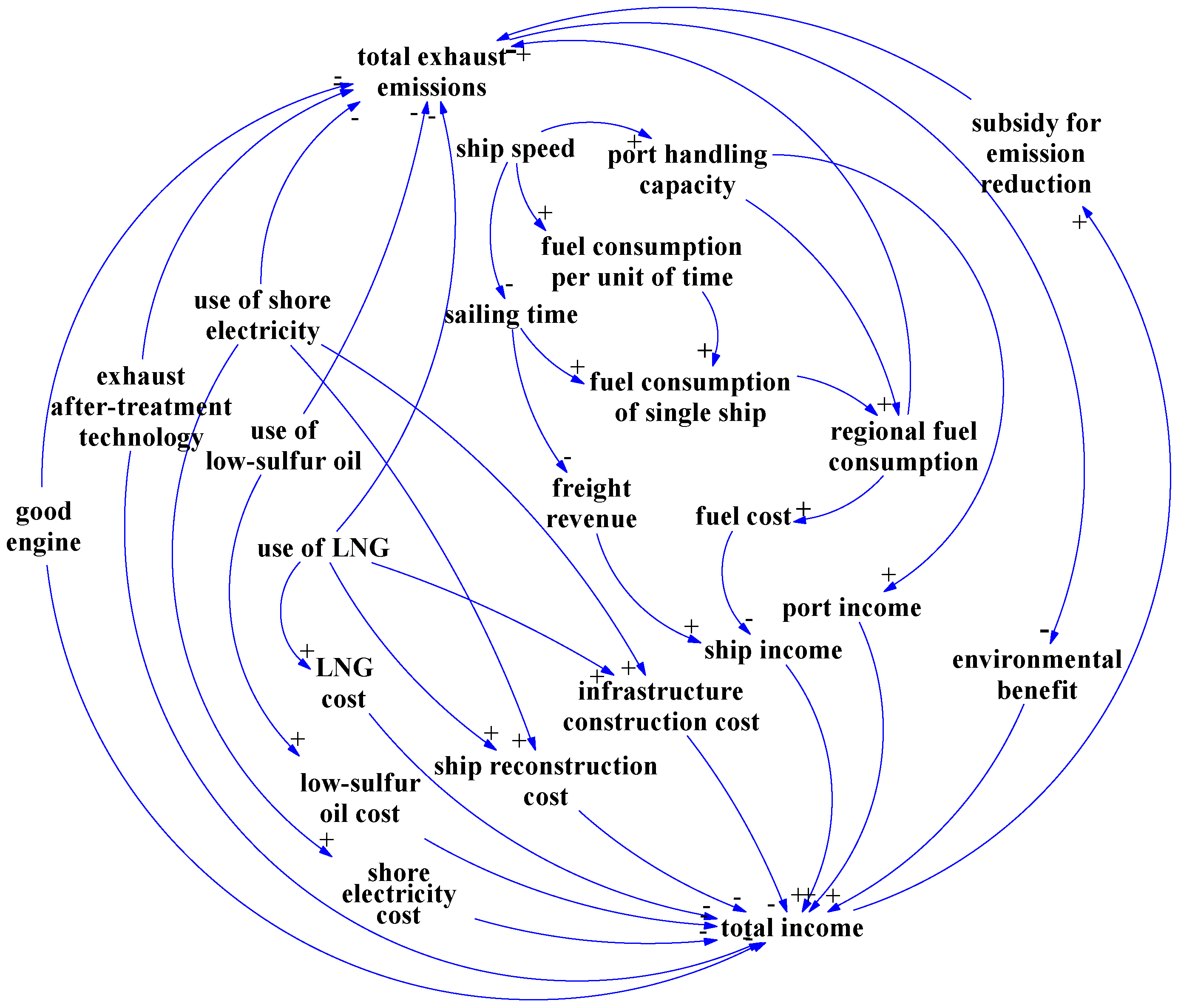
A Causal-loop diagram is an important tool for representing and visualizing the feedback structure of a system. Causal-loop diagram contains a number of feedback loops and variables, and these variables are connected with arrows to reflect the casual relationships. Each feedback loop has its polarity, some are “+”, and the others are “−”, showing how the relative variables will change once a variable changes. SD theory was used to determine the casual relationships among the elements within the sustainable ecosystem, shown in Figure 2.
The interaction between two variables is represented by a causal connection, which is an arrow running from the “cause” to the “effect”) and a polarity, which is indicated by a “+”or “−”. The positive polarity (“+”) on a causal arrow indicates that perturbations in the “causal” variable will result in perturbations in the same direction in the “effect” variable on the assumption that all else in the system is held constant. Similarly, a negative polarity (“−”) indicates that perturbations in the “causal” variable will result in perturbations in the opposite direction in the effect variable, also on the assumption that all else in the system is held constant. [46] Then feedback loops, including the positive feedback loops (reinforcing feedback loops) and negative feedback loops (balancing feedback loops) can be created by the causal relationships. The main feedback loops in the causal loop diagram of the sustainable ecosystem are listed as follows:
- (1)
- Positive feedback loop (Reinforcing feedback loop):
- R1:
- Ship speed → port handling capacity → port income → total income
- (2)
- Negative feedback loop (Balancing feedback loop):
- R2:
- Ship speed → fuel consumption per unit of time of single ship → fuel consumption of single ship → regional fuel consumption → fuel cost → ship income → total income
- R3:
- Ship speed → sailing time → freight revenue → ship income → total income
- R4:
- Ship speed → sailing time → fuel consumption of single ship → regional fuel consumption → total ship exhaust emissions
- R5:
- Use of shore electricity → total ship exhaust emissions
- R6:
- Use of low-sulfur oil → total ship exhaust emissions
- R7:
- Use of LNG → total ship exhaust emissions
- R8:
- Good engine → total ship exhaust emissions
- R9:
- Exhaust after-treatment → total ship exhaust emissions
- R10:
- Total ship exhaust emission → environmental benefits → total income
It can be seen that there are mainly ten feedback loops in the casual loop diagram of the sustainable ecosystem. The first loop R1, which is the only positive feedback loop, includes four variables and the causality of this loop indicates that: if ship speed increases, the port handling capacity will increase, which will bring more port income, then the total income will increase as well. Loops from R2 to R9 are all negative feedback loops. R2 includes seven variables and the causality of this loop indicates that if ship speed increases, the fuel consumption of the single ship for per unit of time will increase, then the regional fuel consumption will increase, which will bring more fuel cost, so the ship income will decrease, then the total income will decrease as well. R3 includes five variables and the causality of this loop indicates that if the ship speed increase, the sailing time of a voyage will be shortened, which will bring more freight revenue, so there will be more ship income, then the total income will increase. There are also five variables in R4 and its causality indicates that shorter sailing time will produce fewer fuel consumption, and there will be less exhaust emissions from ships. R5 to R9 all include two variables and their causalities indicate that use of shore electricity, low-sulfur oil, LNG, using good engine and application of exhaust after-treatment technology all can decrease the total exhaust emissions. R10 includes three variables and the causality of this loop indicates that if the total exhaust emissions decrease, more environmental benefits will be produced, and then the total income will increase. These ten feedback loops are not independent; they interrelated with each other to construct the whole complicated system. To better analyze the intrinsic mechanism of the system, we need further supplement the variables and divide the variables into different sorts, then establish mathematical equations to quantitatively describe the relationships among different variables.
3.2. Stock-Flow Diagram
A causal loop diagram can only describe the basic aspects of a feedback structure, but is unable to show the distinctions among different sorts of variables. A stock-flow diagram can make up for this deficiency. The basic elements in the stock-flow diagram include state variable, rate variable, auxiliary variable, and constant. A stock-flow diagram of the sustainable ecosystem details the causal relationships among different variables in this system, which can be shown in Figure 3. It should be noted that in the diagram, some variables are depicted in the shorter forms. The explanations for the shorter forms are as follows: LF is the load factor, EF is the emission factor, MS is the maximum service speed, P is the rated power, ME is the main engine, AE is the auxiliary engine, LSO is the low-sulfur oil, D is the voyage distance, SE is the shore electricity, and ERC is the emission reduction coefficient.
In this diagram, the variables in the box are state variables, the variables under the arrows are rate variables, and others are auxiliary variables and constants. The value of each stock variable, which is an accumulated value over time, is the difference value of its inflow volume and outflow volume. In this diagram, five variables are represented as stock variables, which are “total fuel consumption”, “total LNG consumption”, “total low-sulfur oil consumption”, “total exhaust emissions” and “total income”. Flow variables include the inflow variables and outflow variables, which reflect the change rate of the stock variables’ values. In this diagram, six variables are represented as flow variables. For example, for “total income”, which is a stock variable, its inflow variable is the increase of income and its outflow variable is the decrease of income. If the increased amount is higher than the decreased amount, then the total income will increase, while if the increased amount is less than the decreased amount, then the total income will decrease. Auxiliary variables are the intermediate variables between the stock variables and the flow variables. In the diagram, there are quantity of auxiliary variables, which are indispensable in detailing and describing the intrinsic mechanism within the system. For example, the auxiliary variable “low-sulfur oil cost” is directly related with the “total low-sulfur oil consumption”, which is a stock variable, and it will also influence the “decrease of income”, which is a flow variable. Constants are the system parameters with invariable values, such as the price of different kinds of energy, the energy consumption ratio, the engine power, the emission factor, etc., we need to determine the values of the constants based on related materials and field investigation, then input them into the model. Moreover, we should establish the mathematical equations to quantitatively describe the relationships among different variables.
3.3. Establishment of the Variable Equations
Ship traffic volume, total fuel consumption, total exhaust emissions and total income are the main variables in the stock-and-flow diagram of the sustainable ecosystem, suggesting complex patterns of interactions among the variables. Ship traffic volume is one of the main influencing factors of the total amount of fuel consumption, and can further influence the amount of exhaust emissions. Each of these factors and their equations will be discussed in turn.
3.3.1. Ship Traffic Volume
Supposing that the cargo handling equipment on the port is enough to support the increasing number of ships attempting to visit the port, that is, the ship traffic volume of the port is not limited by the port capacity. Under this assumption, the number of ships passing the port within the same time period will certainly increase with the increasing of ship speed. Then, the ship traffic volume in the region can be calculated as follows:
In Equation (1), is the ship traffic volume; is the allowed number of ships which can navigate in parallel in the cross section of the channel; is the ship speed, km/h; is number of days during which ships are in navigation; is the navigation time each day, h/day; is the length of the ship, m; and is the spacing coefficient among ships in the region.
3.3.2. Turnover Volume of Freight Transport
Based on the calculation of ship traffic volume, the turnover volume of freight transport can be calculated as follows:
In Equation (2), is the turnover volume of freight transport, t; is the average dead weight tonnage of the ship, t; and is the ship traffic volume.
3.3.3. Total Fuel Consumption
The fuel consumption of single ship can be calculated as follows (Xie, 2009 [2]):
In Equation (3), is the fuel consumption of single ship, g; represents different engine type; is the rated power of engine , ; is the load factor of engine ; is the running time of engine , h; and is the fuel consumption rate of engine , . The load factor of the ship main engine can be calculated as follows:
In Equation (4), is the load factor of the ship main engine; is the maximum service speed of the ship, km/h, which can be acquired by multiplying 1.064 on the basis of the speed provided by Lloyd’s database [32]. The load factor of the ship auxiliary engine was acquired from a research report of US Environment and Protection Association (USEPA) [32].
When the ship is in navigation status, both the main engine and auxiliary engine consume oil, while when the ship is in anchoring or berthing status, the main engine stops working, and its fuel consumption can be ignored. When in berthing status, if the shore electricity is used, then both the main and auxiliary engine of the ship stop working and have no fuel consumption. Based on this analysis, Equation (3) can be detailed as follows:
In Equation (5), and represent the fuel consumption of the main and auxiliary engine, respectively, for the single ship, g; and represent the rated power of the main and auxiliary engine, respectively, kw; and represent the working time of main and auxiliary engine, respectively, h; and and represent the fuel consumption rate of main and auxiliary engine, respectively, . Using to represent the sailing time, to represent the anchoring time, and to represent the berthing time, then and .
Then, the total fuel consumption in the region can be represented as:
In Equation (6), is the total amount of fuel consumption in the region, g; is the amount of fuel consumption for single ship, g; is the ship traffic volume; and is the consumption ratio of fuel oil.
3.3.4. Total Exhaust Emissions
In reference with the research methods of USEPA [32], the total exhaust emissions originating from ships in the region can be calculated as follows:
In Equation (7), is the total amount of exhaust emissions, g; , , and are the consumption amounts of fuel oil, LNG and low-sulfur oil, respectively. , , and are the emission factors of fuel oil, LNG and low-sulfur oil, respectively. and are the emission reduction coefficients for the use of good engine and application of exhaust after-treatment technology, respectively.
3.3.5. Total Income
The regional total income can be calculated as follows:
In Equation (8), is the total income; is the port income, which represents the port tariffs paid to the port by shippers; is the ship income, which is the difference value between the freight income and related cost including the fuel cost and port tariffs; is the LNG cost; is the low-sulfur oil cost; is the construction cost of relevant infrastructures; is the ship reconstruction cost; is the cost of good engine; and is the cost of exhaust after-treatment. It should be noted that health and environmental benefits brought by the reduction of ship exhaust emissions are also part of the total income, and, in this figure, we use the variable pollution loss to represent the economic loss due to the bad effects on the health and environment caused by ship exhaust emissions. However, the pollution loss is related with many factors, such as the diffusion of ship exhaust emissions, how ship exhaust emissions affect the human health, cost of pollution abatement, etc., which are hard to quantitatively calculate based on acquired data. Therefore, here the pollution loss has not been taken into consideration in the calculation of the total income.
After determining the mathematical equations, relationships among different variables in the sustainable ecosystem can be quantified and the complex intrinsic mechanism within the entire system can be intensively described. On this basis, simulation experiments can be made using SD simulation software VENSIM (Ventana Simulation) to verify the availability of the model and predict the potential environmental and economic development in the region. VENSIM, which was developed by the Ventana Systems Inc. in America, is the most commonly-used modeling and simulating software in the SD research field. As a visualized modeling tool, it can be applied to the simulation, analysis and optimization of complicated models, and can be used for developing, analyzing and packaging dynamic feedback loops within the models.
4. Case Study
In this paper, Qingdao port in China is taken as the study area. As the important economic center and port city in the east coast of China, the port economy in Qingdao is also developing fast, which has brought the increasing amount of ship exhaust emissions. From the year of 2002, Qingdao environmental protection agency has cooperated with SIDA (Swedish International Development Cooperation Agency) to develop the management system of the environmental air quality in Qingdao. Combining this project, the emission inventory of the marine traffic sources in Qingdao port has been established, and the proportion of emissions originating from different sources have been quantified. Then based on GIS (Geographical Information System), the diffusion model of the exhaust emissions was further established, which can be applied to the spatial simulation and measurement of the ship exhaust emissions [47]. All these researches have made Qingdao port an ideal location for our study. The main data sources are as follows: Report on China Shipping Development (2014), Statistical yearbook of Qingdao (2014) and related materials provided by Qingdao port.
4.1. Historical Validation
Turnover volume of freight transport is one of the main variables in the sustainable ecosystem. Considering the variation of data completeness for different variables across the dataset, the historical date of the cargo throughput and turnover volume of freight transport of Qingdao port from 2005 to 2014 were selected to make comparison with the simulated values. The historical verification results for Qingdao port are shown in Table 1.
It can be seen in Table 1 that both the simulation results of the cargo throughput and turnover volume of freight transport of Qingdao port from 2005 to 2014 are close to the historical data, with errors between −6% to 6%, confirming that our model is effective. The historical data of the total ship exhaust emissions and the total income are not complete, so the historical data of these two variables are not selected to make validation. However, the minor errors between the simulated cargo throughput and corresponding historical values as well as the minor errors between the simulated turnover volume of freight transport and corresponding historical values can validate that this model is effective and can perform well; therefore, we can make further simulation experiments using this model to predict the future environmental and economic development of Qingdao port under different scenarios.
4.2. Experimental Design
After verifying the effectiveness of the model, we can use this model to simulate the reduction of ship exhaust emissions when different measures are taken. As described in the part of introduction, there are different measures of mitigating ship exhaust emissions, such as speed reduction, improving the energy consumption structure, using shore electricity during berth, and applying engine improvement and exhaust after-treatment technologies. Therefore, we can take the parameters such as the ship speed, consumption ratio of different kinds of energy, whether shore electricity is used and whether engine improvement technology or exhaust after-treatment technology is used as the controlling variables to simulate the effects of different measures on the reduction of ship exhaust emissions as well as the economic development in the region. It should be noted that, in the combustion of LNG, methane slip will also cause atmospheric pollution. However, the leakage of methane into the atmosphere contains many factors such as the leakage amount, leakage rate, the diffusion of the leaked methane, etc. which are hard to quantitatively calculate. Therefore, in this paper, influences of methane slip on the atmosphere are not considered. Considering the combination of different emission mitigation measures, we have designed 15 different schemes, which can be shown in Table 2, to simulate the total exhaust emissions and total income under different schemes.
5. Simulation Results
Simulation is made to predict the exhaust emissions and economic income trends for the city of Qingdao port over 2015–2025, and the simulation time-step is set as one year. To better analyze the simulation results, different groups of scenarios were designed to analyze the effects of different schemes and measures. These scenarios include speed reduction, improvement of energy consumption structure, use of shore electricity, application of engine improvement technology and exhaust after-treatment technology. The last scenario examines the effects of a combination of all of these measures, that is a multi-measure scenario.
5.1. Effects of Speed Reduction
To analyze the effect of speed reduction, we choose the ship speed as the experimental variable and keep other variables the same, to design four tests with different ship speed. The ship speed from Test 1 to Test 4 is 26 km/h, 22 km/h, 18 km/h, 12 km/h, respectively. The simulation results of Test 1 to Test 4 are as follows (Figure 4).
It can be seen in Figure 5 that, when the ship speed is 18 km/h, the exhaust emissions are the fewest and the income is the highest. This indicates that reducing the ship speed from 26 km/h to 18 km/h can decrease fuel consumption, mitigate exhaust emissions and increase the total income, while if the ship speed was reduced from 18 km/h to 12 km/h, the fuel consumption will increase, and there will be more exhaust emissions and lower income. The reason is that the fuel consumption is not in linear relationship with the ship speed. On the one hand, reduction of ship speed can decrease the fuel consumption per unit of time, which is in positive correlation with the total fuel consumption; on the other hand, it will prolong the sailing time, which is in negative correlation with the total fuel consumption. Therefore, there exists an optimal speed value which can produce the fewest fuel consumption, the fewest exhaust emissions, as well as the highest economic income.
5.2. Effects of the Energy Consumption Structure Improvement
5.2.1. Use of Low-Sulfur Oil or LNG
To compare the variation trends of exhaust emissions and economic benefit when different kinds of energy are used, we choose the energy consumption ratio as the experimental variable and keep other variables to be the same. In Test 3, the consumption ratio of fuel is 100%; in Test 6, the consumption of low-sulfur oil is 100%; and, in Test 7, the consumption of LNG is 100%. The simulation results of these three tests are as follows (Figure 5).
The simulation results show that when the consumption ratio of fuel is 100%, the amount of exhaust emissions is the most and the total income is the lowest, and using low-sulfur oil or LNG can greatly mitigate the exhaust emissions and increase the total income. When the consumption ratio of LNG is 100%, the emission reduction effect is the best, and the total income is the highest as well. This is because, compared with consuming fuel oil, consuming low-sulfur oil can greatly reduce the amount of SOX and PM emissions, thus the total exhaust emissions can be reduced. For the clean energy LNG, its main component is methane, of which the combustion products are only CO2 and H2O; therefore, the total amount of exhaust emissions can be greatly reduced if LNG is used as the alternative energy. Besides, the reduction of emissions will produce great environmental benefits, so the total income will increase.
5.2.2. Combination Use of Low-Sulfur Oil and LNG
To analyze the effects when different ratios of fuel oil, low-sulfur oil and LNG are consumed, we take the consumption ratio of these three different kinds of energy as the controlling variable, at the same time, other variables are kept to be the same. In Test 5, the consumption ratios of fuel oil, low-sulfur oil and LNG are 20%, 40% and 40%, respectively; in Test 8, the ratios are 0%, 50% and 50%, respectively; in Test 9, the ratios are 0%, 20% and 80%, respectively; and in Test 10, the ratios are 0%, 80% and 20%, respectively. The comparison results of these four tests are as follows (Figure 6).
From the simulation results, we can see that, among these four tests, when the consumption ratios of fuel oil, low-sulfur oil and LNG are 20%, 40% and 40%, respectively, the amount of exhaust emissions is the most, and the total income is the lowest. In Tests 8–10, the consumption ratio of fuel oil is further decreased to 0, and then the exhaust emissions decreased and the total income increased compared with Test 5. Among these three tests, when the consumption ratios of low-sulfur oil and LNG are 20% and 80%, the amount of exhaust emissions is the fewest, and the total income is the highest; when the ratios of low-sulfur oil and LNG are 50% and 50%, the amount of exhaust emissions is the second fewest, and the total income is the second highest; and when the ratios of low-sulfur oil and LNG are 80% and 20%, the amount of exhaust emissions is the third fewest, and the total income is the third highest. Therefore, improving the energy consumption structure by decreasing the fuel consumption ratio and increasing the consumption ratios of low-sulfur oil and LNG can decrease the exhaust emissions and increase the economic income. When only low-sulfur oil and LNG are consumed, the higher the LNG consumption ratio is, the fewer the exhaust emissions and the higher the total income will be.
5.3. Effects of the Shore Electricity Use
To analyze the effects of using shore electricity, whether shore electricity is used during the berthing status is set as the experimental variable, and other variables are kept to be the same. In Test 5, shore electricity is used in the berthing status, while, in Test 11, no shore electricity is used. The comparison results of Test 5 and Test 11 are as follows (Figure 7).
The simulation results show that using shore electricity in the berthing status can mitigate the exhaust emissions and increase the income, and, from longer time scale, the effect is more obvious. The reason is that, in the berthing status, the main engine stops working while the auxiliary engine reaches its load peak, at this time, if shore electricity is used to power the operation of the shipboard equipment instead of the combustion of the auxiliary engine, then the fuel consumption in the berthing status will be greatly decreased, and will produce less exhaust emissions. As the shore electricity cost is lower than the fuel cost in the berthing status, the economic income will increase as well.
5.4. Effects of Using Engine Improvement Technology and Exhaust After-Treatment Technology
To analyze the effects of the application of engine improvement and exhaust after-treatment technologies, whether engine improvement technology is applied and whether exhaust after-treatment technology is applied are taken as the experimental variables, at the same time, other variables are kept to be the same. In Test 5, neither of these two technologies is used; in Test 12, only engine improvement technology is used; in Test 13, only exhaust after-treatment technology is used; and, in Test 14, both of these two technologies are used. The comparison results of these four tests are as follows (Figure 8).
The simulation results show that both the application of engine improvement technology and exhaust after-treatment technology can mitigate the exhaust emissions, and when both of these two technologies are used, the amount of exhaust emissions is the fewest and the economic income is the highest. Comparing the results of Test 12 and Test 13, it can be indicated that compared with applying exhaust after-treatment technology, the application of engine improvement technology can get larger mitigation magnitude of exhaust emissions, and produce higher economic income.
5.5. Effects of the Combination of Multi Measures
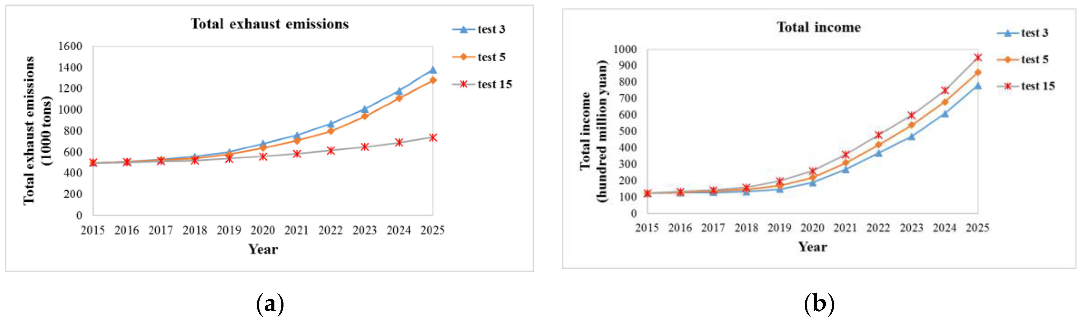
To analyze the effects of the combination of different measures, Tests 3, 5 and 15 are compared: in Test 3, only the ship speed is reduced; in Test 5, the energy consumption structure is improved on the basis of Test 3; and, in Test 15, the other emission mitigation measures including the shore-electricity, engine improvement technology and exhaust-after treatment technology are used on the basis of Test 5. The comparison results of these three tests are as follows (Figure 9).
The comparison results show that, among these three tests, the amount of the total exhaust emissions of Test 3, in which only the measure of speed reduction is used, is the most; that of Test 5, in which the measures of speed reduction and energy consumption structure improvement are used, is the second most; and that of Test 15, in which different kinds of emission mitigation measures are used, is the least. Accordingly, the total income of Test 3 is the lowest, that of Test 5 is second lowest, and that of Test 15 is the highest. Therefore, it is indicated that using the combination emission mitigation measures can achieve fewer exhaust emissions and higher economic income compared with using a single measure.
6. Discussion and Conclusions
This paper presents a System Dynamics model based on relations between regional exhaust emissions and economic benefits with Qingdao port as a case study, the aim of which is to analyze the effects of different measures to promote the development of the sustainable ecosystem. According to the simulation results for period of 2015–2025 under different scenarios, the following conclusions can be drawn:
- (1)
- Under the market environment that the supply exceeds demand, ship speed should be suitably reduced to achieve greater economic and environmental benefits. The reduction extent should not be too large, the optimal ship speed value produces the fewest exhaust emissions and the highest economic income. If a ship speed is too low, the sailing time will be greatly prolonged, and the amount of exhaust emissions will increase, thus the total income will be lower.
- (2)
- Improvement of the energy consumption structure is an effective measure to promote the development of the sustainable ecosystem. Schemes with different energy consumption structures were designed, simulation results show that increasing the consumption ratio of low-sulfur oil and LNG can greatly mitigate the exhaust emissions to increase the environmental benefits.
- (3)
- Using shore electricity in the berthing status is also an effective measure for the promotion of the sustainable ecosystem. In the berthing status, the main engine of the ship stops working while the auxiliary engine reaches its load peak. If shore electricity is used as an alternative energy source during berthing, ship exhaust emissions will be greatly reduced and the total income will increase.
- (4)
- Application of engine improvement and exhaust after-treatment technologies could also greatly mitigate exhaust emissions, increase the total income and promote the development of the sustainable ecosystem. Moreover, a combination of multi measures could achieve even better effects compared with just applying a single measure. Obviously, the effect of exhaust emission reduction is the best when all kinds of measures are applied, including the speed reduction, improvement of energy consumption structure, using shore electricity, applying engine improvement technology and exhaust after-treatment technology.
The research results presented in this paper could be a model for regional sustainable development. By changing the numeric values of certain parameters, the model can be further applied to analyze the decision-making for the development of other regions and cities other than the study area Qingdao port in China.
However, there still exist some problems and limitations:
- (1)
- The data used in the simulation experiments were limited, incomplete and not comprehensive enough to completely validate the effectiveness of the proposed model. In later studies, we will acquire more detailed materials and thorough information in order to make a more reasonable validation of the model.
- (2)
- There exist ambiguity and uncertainties in the establishment of variable equations and in the determination of parameter values, as the particularities of ships of different types and different routes were not considered in this research. Future researches will incorporate additional detailed data to further improve the model.
Acknowledgments
The work described in this presentation is supported by the National Science Foundation of China (NSFC) through Grant No. 51679180 and Double First-rate Project of WUT as well as the Graduate Student Innovation Funds Project of Wuhan University of Technology, China (Grant No. 2015-zy-107). The author thanks the groups of National Engineering Research Center for Water Transport Safety and Hubei Key Laboratory of Inland Shipping Technology, China for supporting the related investigation.
Author Contributions
Xiaoqiao Geng and Yuanqiao Wen conceived and designed the experiments; Xiaoqiao Geng and Chunhui Zhouperformed the experiments and analyzed the data; Yuanqiao Wen and Changshi Xiao contributed analysis tools; and Xiaoqiao Geng and Chunhui Zhou wrote the paper.
Conflicts of Interest
The authors declare no conflict of interest.
References
- Smith, T.W.P.; Jalkanen, J.P.; Anderson, B.A. Third IMO GHG Study; International Maritime Organization (IMO): London, UK, 2014. [Google Scholar]
- Xie, G.M. Analysis on Economy and Emission Change of Navigation at Reduced Speed. Master’s Thesis, Dalian Maritime University, Dalian, Liaoning, China, 2009. [Google Scholar]
- Woo, J.-K.; Moon, D.S.-H. The effects of slow steaming on environmental performance in liner shipping. Marit. Policy Manag. 2014, 41, 176–191. [Google Scholar] [CrossRef]
- Winebrake, J.J.; Corbett, J.J.; Green, E.H. Mitigating the health impacts of pollution from oceangoing shipping: An assessment of low-sulfur fuel mandates. Environ. Sci. Technol. 2009, 43, 4776–4782. [Google Scholar] [CrossRef] [PubMed]
- Peng, H.K. LNG Fuel Powered Ship Transforms Pilot Job Analysis. China Mar. 2012, 10, 47–49. [Google Scholar]
- Jia, S.Y. Study of Reduction of GHG Emission from Ships by Shore Power. Master’s Thesis, Dalian Maritime University, Dalian, Liaoning, China, 2009. [Google Scholar]
- Yang, J.; Cheng, Z. Research on Emissions After treatment in Diesel Engines. Intern. Combust. Engines 2007, 4, 45–48. [Google Scholar]
- He, Y.Y.; Tan, X. Research on Policy Influences on regional Low-Carbon Development Based on System Dynamics—Case Study on China. J. Tianjin Univ. (Soc. Sci.) 2013, 15, 507–511. [Google Scholar]
- Dai, X. Study on Industrial Structural Upgrading and CO2 Emissions in China Based on System Dynamics. Master’s Thesis, Tianjin University, Tianjin, China, 2013. [Google Scholar]
- Shi, T. Simulation and Optimization of Carbon Emission System Based on System Dynamics. Master’s Thesis, North China Electric Power University, Beijing, China, 2013. [Google Scholar]
- Youssef, A.A. Asset Management Tools for Municipal Infrastructure Considering Interdependency and Vulnerability. Ph.D. Thesis, Concordia University, Montréal, QC, Canada, 2015. [Google Scholar]
- Fan, T.S. Research on Development Pattern of Low-carbon Economy Based on System Dynamics Model: A Case of Fujian. East China Econ. Manag. 2013, 27, 12–16. [Google Scholar]
- Feng, Y.Y.; Chen, S.Q.; Zhang, L.X. System dynamics modeling for urban energy consumption and CO2 emissions: A case study of Beijing, China. Ecol. Model. 2013, 252, 44–52. [Google Scholar] [CrossRef]
- Liu, X.; Mao, G.; Ren, J.; Li, R.Y.M.; Guo, J.; Zhang, L. How might China achieve its 2020 emissions target? A scenario analysis of energy consumption and CO2 emissions using the system dynamics model. J. Clean. Prod. 2015, 103, 401–410. [Google Scholar] [CrossRef]
- Qin, Z.; Zhang, J.E.; Luo, S.M. Prediction of energy consumption and CO2 emission by system dynamics approach. Chin. J. Eco-Agric. 2008, 16, 1043–1047. [Google Scholar] [CrossRef]
- Robalino-López, A.; Mena-Nieto, A.; García-Ramos, J.E. System dynamics modeling for renewable energy and CO2 emissions: A case study of Ecuador. Energy Sustain. Dev. 2014, 20, 11–20. [Google Scholar] [CrossRef]
- Rusiawan, W.; Tjiptoherijanto, P.; Suganda, E.; Darmajanti, L. System Dynamics Modeling for Urban Economic Growth and CO2 Emission: A Case Study of Jakarta, Indonesia. Procedia Environ. Sci. 2015, 28, 330–340. [Google Scholar] [CrossRef]
- Abbas, K.A.; Bell, M.G.H. System dynamics applicability to transportation modelling. Transp. Res. Part A 1994, 28A, 373–400. [Google Scholar]
- Blumberga, D.; Blumberga, A.; Barisa, A.; Rosa, M. System Dynamic Modeling of Low Carbon Strategy in Latvia. Energy Procedia 2014, 61, 2164–2167. [Google Scholar] [CrossRef]
- Liu, S.; Chen, S.; Liang, X.; Mao, B. Analysis of Transport Policy Effect on CO2 Emissions Based on System Dynamics. Adv. Mech. Eng. 2015, 7, 323819. [Google Scholar] [CrossRef]
- Engelen, S.; Meersman, H.; van de Voorde, E. Using system dynamics in maritime economics: An endogenous decision model for shipowners in the dry bulk sector. Marit. Policy Manag. 2006, 33, 141–158. [Google Scholar] [CrossRef]
- Tang, L.M.; Chen, Y.; Liu, S.H. System dynamics model of low-carbon development of Chinese shipping industry under international carbon emission market mechanism. J. Shanghai Marit. Univ. 2015, 36, 25–30. [Google Scholar]
- Dace, E.; Muizniece, I.; Blumberga, A.; Kaczala, F. Searching for solutions to mitigate greenhouse gas emissions by agricultural policy decisions—Application of system dynamics modeling for the case of Latvia. Sci. Total Environ. 2015, 527, 80–90. [Google Scholar] [CrossRef] [PubMed]
- Kim, K.S.; Cho, Y.J.; Jeong, S.J. Simulation of CO2 emission reduction potential of the iron and steel industry using a system dynamics model. Int. J. Precis. Eng. Manuf. 2014, 15, 361–373. [Google Scholar] [CrossRef]
- Ansari, N.; Seifi, A. A system dynamics model for analyzing energy consumption and CO2 emission in Iranian cement industry under various production and export scenarios. Energy Policy 2013, 58, 75–89. [Google Scholar] [CrossRef]
- Han, J.; Hayashi, Y. A system dynamics model of CO2 mitigation in China’s inter-city passenger transport. Transp. Res. Part D 2008, 13, 298–305. [Google Scholar] [CrossRef]
- Trappey, A.J.C.; Trappey, C.; Hsiao, C.T.; Jerry, J.R.O.; Li, S.J.; Chen, L.W.P. An evaluation model for low carbon island policy: The case of Taiwan’s green transportation policy. Energy Policy 2012, 45, 510–515. [Google Scholar] [CrossRef]
- Saysel, A.K.; Hekimoğlu, M. Exploring the options for carbon dioxide mitigation in Turkish electric power industry: System dynamics approach. Energy Policy 2013, 60, 675–686. [Google Scholar] [CrossRef]
- Horng, J.J.; Lee, R.F.; Liao, K.Y. Using Stella System Dynamic Model to Analyze Greenhouse Gases’ Emission from Solid Waste Management in Taiwan; Department of Energy, Environmental Management Science Program: Washington, DC, USA, 2004.
- Cai, W. Calculating Methods for Ship Air Pollutants. J. Wuhan Univ. Technol. (Transp. Sci. Eng.) 2004, 28, 485–487. [Google Scholar]
- Wan, L.; He, L.Y.; Huang, X.F. Progress in research of air pollution emissions from ships. Environ. Sci. Technol. 2013, 5, 013. [Google Scholar]
- Browning, L.; Bailey, K. Current Methodologies and Best Practices for Preparing Port Emission Inventories; ICF Consulting report to Environmental Protection Agency; US EPA: Washington, DC, USA, 2006. [Google Scholar]
- Goldsworthy, L.; Goldsworthy, B. Modelling of ship engine exhaust emissions in ports and extensive coastal waters based on terrestrial AIS data—An Australian case study. Environ. Model. Softw. 2015, 63, 45–60. [Google Scholar] [CrossRef]
- Zhu, Q.R.; Liao, C.H.; Liu, J.J.; Zhang, Y.B. Research on the air pollutant emission in the typical river ports and harbors, Guangdong. J. Saf. Environ. 2015, 3, 045. [Google Scholar]
- Tan, J.W.; Song, Y.N.; Ge, Y.S.; Li, J.Q.; Li, L. Emission inventory of oceangoing vessels in Dalian Coastal area. Res. Environ. Sci. 2014, 12, 007. [Google Scholar]
- Ye, S.Q.; Zheng, J.Y.; Pan, Y.Y.; Wang, S.S.; Lu, Q.; Zhong, L.J. Marine emission inventory and its temporal and spatial characteristics in Guangdong Province. Res. Environ. Sci. 2014, 34, 537–547. [Google Scholar]
- Jin, T.S.; Yin, X.G.; Xu, J.; Yang, L.; Ge, W.H.; Ju, M.T. Air pollutants emission inventory from commercial ships of Tianjin Harbor. Mar. Environ. Sci. 2009, 28, 623–625. [Google Scholar]
- Fu, Q.Y.; Shen, Y.; Zhang, J. On the ship pollutant emission inventory in Shanghai port. J. Saf. Environ. 2012, 5, 57–63. [Google Scholar]
- Ye, S.Q. Study of Characteristics Emission and Its Impact on of Marine Vessel Regional Air Quality of the Pearl River Delta Region. Master’s Thesis, South China University of Technology, Guangzhou, Guangdong, China, 2014. [Google Scholar]
- Yin, P.L.; Ye, S.Q.; Wang, S.S. Marine Emission Inventory and Its Temporal and Spatial Characteristics in the city of Shenzhen. Environ. Sci. 2015, 4, 014. [Google Scholar]
- Kesgin, U.; Vardar, N. A study on exhaust gas emissions from ships in Turkish Straits. Atmos. Environ. 2001, 35, 1863–1870. [Google Scholar] [CrossRef]
- Yau, P.S.; Lee, S.C.; Corbett, J.J. Estimation of Ship Emission of Ocean-going Vessels in Hong Kong. Sci. Total Environ. 2012, 431, 299–306. [Google Scholar] [CrossRef] [PubMed]
- Jalkanen, J.P.; Brink, A.; Kalli, J.; Pettersson, H.; Kukkonen, J.; Stipa, T. A modelling system for the exhaust emissions of marine traffic and its application in the Baltic Sea area. Atmos. Chem. Phys. 2009, 9, 9209–9223. [Google Scholar] [CrossRef]
- Song, S.K.; Shon, Z.H. Current and future emission estimates of exhaust gases and particles from shipping at the largest port in Korea. Environ. Sci. Pollut. Res. 2014, 21, 6612–6622. [Google Scholar] [CrossRef] [PubMed]
- Adamo, F.; Andria, G.; Cavone, G.; Capuab, C.D.; Lanzollaa, A.M.L.; Morellob, R.; Spadavecchiaa, M. Estimation of ship emissions in the port of Taranto. Measurement 2014, 47, 982–988. [Google Scholar] [CrossRef]
- Stepp, M.D.; Winebrake, J.J.; Hawker, J.S.; Skerlos, S.J. Greenhouse gas mitigation policies and the transportation sector: The role of feedback effects on policy effectiveness. Energy Policy 2009, 37, 2774–2787. [Google Scholar] [CrossRef]
- Liu, J.; Wang, J.; Song, C.Z.; Qin, J.J. The Establishment and Application of Ship Emissions Inventory in Qingdao Port. Environ. Monit. China 2011, 3, 50–53. [Google Scholar]
Figure 1.
Framework of the regional sustainable ecosystem.
Figure 2.
Causal loop diagram of the sustainable ecosystem.

Figure 3.
Stock-flow diagram of the sustainable ecosystem.
Figure 4.
Effects of ship speed reduction: (a) total exhaust emissions; and (b) total income.
Figure 5.
Effects of using low-sulfur oil or LNG: (a) total exhaust emissions; and (b) total income.
Figure 5.
Effects of using low-sulfur oil or LNG: (a) total exhaust emissions; and (b) total income.
Figure 6.
Effects of the combination use of low-sulfur oil and LNG: (a) total exhaust emissions; and (b) total income.
Figure 6.
Effects of the combination use of low-sulfur oil and LNG: (a) total exhaust emissions; and (b) total income.
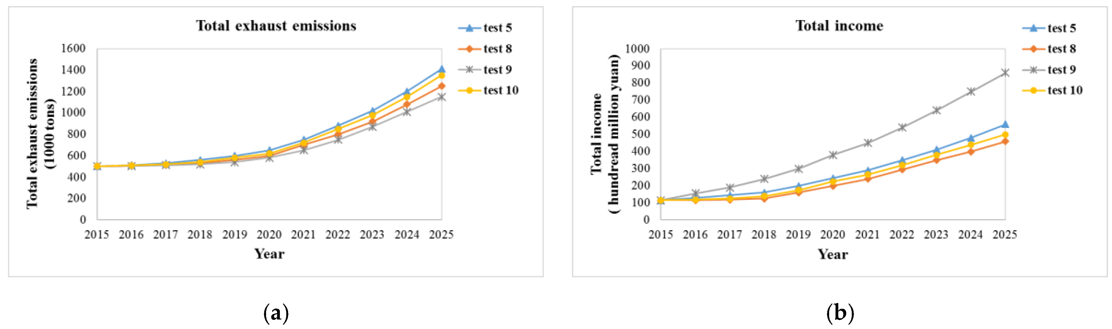
Figure 7.
Effects of the use of shore electricity: (a) total exhaust emissions; and (b) total income.
Figure 7.
Effects of the use of shore electricity: (a) total exhaust emissions; and (b) total income.
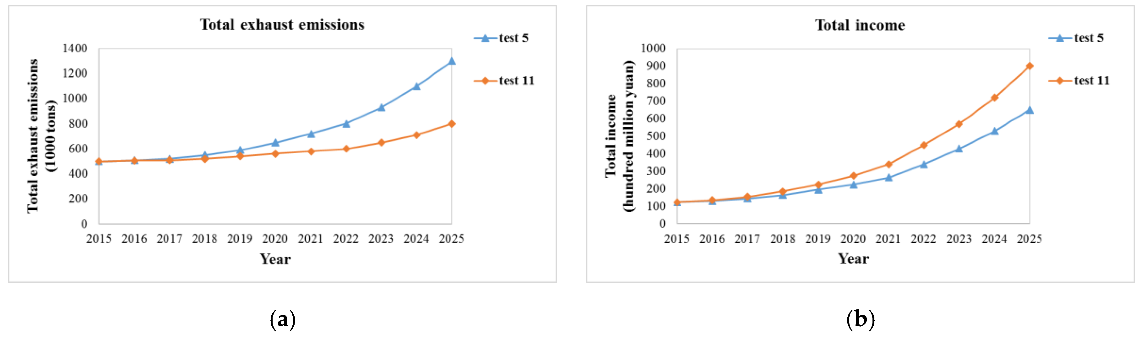
Figure 8.
Effects of applying good engine and exhaust after-treatment: (a) total exhaust emissions; and (b) total income.
Figure 8.
Effects of applying good engine and exhaust after-treatment: (a) total exhaust emissions; and (b) total income.
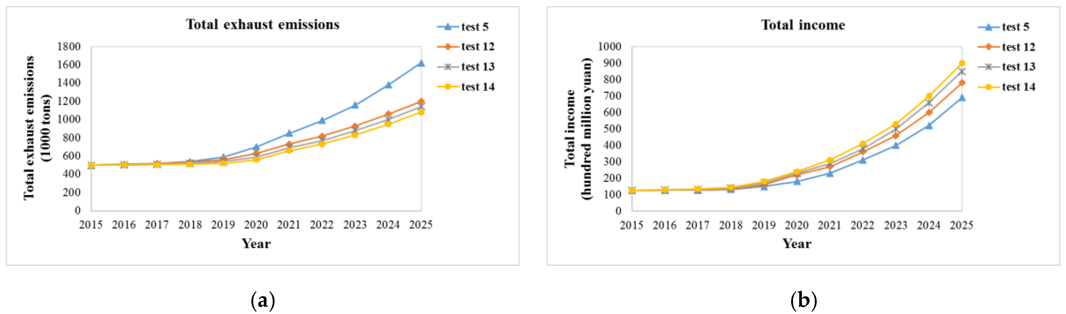
Figure 9.
Effects of the combination of multi measures: (a) total exhaust emissions; and (b) total income.
Figure 9.
Effects of the combination of multi measures: (a) total exhaust emissions; and (b) total income.


Table 1.
Results of historical verification for Qingdao port.
| Year | Cargo Throughput (1000 tons) | Turnover Volume of Freight Transport (100 million ton-km) | ||||
|---|---|---|---|---|---|---|
| True Value | Simulated Value | Error | True Value | Simulated Value | Error | |
| 2005 | 18,727 | 18,727 | 0.00% | 3155 | 3111 | −1.38% |
| 2006 | 22,438 | 21,282 | −5.15% | 3648 | 3667 | 0.51% |
| 2007 | 26,507 | 25,860 | −2.44% | 3279 | 3382 | 3.13% |
| 2008 | 30,029 | 36,820 | −1.34% | 4384 | 4420 | 0.83% |
| 2009 | 31,668 | 29,267 | −2.67% | 3453 | 2506 | 1.55% |
| 2010 | 35,012 | 35,450 | 1.25% | 3073 | 3146 | 2.38% |
| 2011 | 37,971 | 48,103 | 0.78% | 3237 | 3285 | 1.47% |
| 2012 | 41,465 | 38,267 | 2.55% | 1426 | 1439 | 0.89% |
| 2013 | 45,782 | 47,462 | 3.67% | 428 | 425 | −0.66% |
| 2014 | 47,701 | 50,195 | 5.23% | 427 | 429 | 0.52% |
Table 2.
Scenario setting.
| Scenario Number | Ship Speed (km/h) | Consumption Ratio | Whether Use or Not | ||||
|---|---|---|---|---|---|---|---|
| Fuel Oil | Low-Sulfur Oil | LNG | Shore Electricity | Engine Improvement Technology | Exhaust After-Treatment Technology | ||
| 1 | 26 | 100% | 0 | 0 | No use | No use | No use |
| 2 | 22 | 100% | 0 | 0 | No use | No use | No use |
| 3 | 18 | 100% | 0 | 0 | No use | No use | No use |
| 4 | 12 | 100% | 0 | 0 | No use | No use | No use |
| 5 | 18 | 20% | 40% | 40% | No use | No use | No use |
| 6 | 18 | 0 | 100% | 0 | No use | No use | No use |
| 7 | 18 | 0 | 0 | 100% | No use | No use | No use |
| 8 | 18 | 0 | 50% | 50% | No use | No use | No use |
| 9 | 18 | 0 | 20% | 80% | No use | No use | No use |
| 10 | 18 | 0 | 80% | 20% | No use | No use | No use |
| 11 | 18 | 20% | 40% | 40% | Use | No use | No use |
| 12 | 18 | 20% | 40% | 40% | No use | No use | Use |
| 13 | 18 | 20% | 40% | 40% | No use | Use | No use |
| 14 | 18 | 20% | 40% | 40% | No use | Use | Use |
| 15 | 18 | 20% | 40% | 40% | Use | Use | Use |
© 2017 by the authors. Licensee MDPI, Basel, Switzerland. This article is an open access article distributed under the terms and conditions of the Creative Commons Attribution (CC BY) license (http://creativecommons.org/licenses/by/4.0/).
Share and Cite
MDPI and ACS Style
Geng, X.; Wen, Y.; Zhou, C.; Xiao, C. Establishment of the Sustainable Ecosystem for the Regional Shipping Industry Based on System Dynamics. Sustainability 2017, 9, 742. https://doi.org/10.3390/su9050742
AMA Style
Geng X, Wen Y, Zhou C, Xiao C. Establishment of the Sustainable Ecosystem for the Regional Shipping Industry Based on System Dynamics. Sustainability. 2017; 9(5):742. https://doi.org/10.3390/su9050742
Chicago/Turabian StyleGeng, Xiaoqiao, Yuanqiao Wen, Chunhui Zhou, and Changshi Xiao. 2017. "Establishment of the Sustainable Ecosystem for the Regional Shipping Industry Based on System Dynamics" Sustainability 9, no. 5: 742. https://doi.org/10.3390/su9050742
Note that from the first issue of 2016, this journal uses article numbers instead of page numbers. See further details here.