Enhancing Productivity and Resource Conservation by Eliminating Inefficiency of Thai Rice Farmers: A Zero Inefficiency Stochastic Frontier Approach

Abstract

The study first identified fully efficient farmers and then estimated technical efficiency of inefficient farmers, identifying their determinants by applying a Zero Inefficiency Stochastic Frontier Model (ZISFM) on a sample of 300 rice farmers from central-northern Thailand. Next, the study developed scenarios of potential production increase and resource conservation if technical inefficiency was eliminated. Results revealed that 13% of the sampled farmers were fully efficient, thereby justifying the use of our approach. The estimated mean technical efficiency was 91%, implying that rice production can be increased by 9%, by reallocating resources. Land and labor were the major productivity drivers. Education significantly improved technical efficiency. Farmers who transplanted seedlings were relatively technically efficient as compared to those who practised manual and/or mechanical direct seeding methods. Elimination of technical inefficiency could increase output by 8.64% per ha, or generate 5.7–6.4 million tons of additional rice output for Thailand each year. Similarly, elimination of technical inefficiency would potentially conserve 19.44% person-days of labor, 11.95% land area, 11.46% material inputs and 8.67% mechanical power services for every ton of rice produced. This translates into conservation of 2.9–3.0 million person-days of labor, 3.7–4.5 thousand km² of land, 10.0–14.5 billion baht of material input and 7.6–12.8 billion baht of mechanical power costs to produce current level of rice output in Thailand each year. Policy implications include investment into educating farmers, and improving technical knowledge of seeding technology, to boost rice production and conserve scarce resources in Thailand.

1. Introduction

The measurement of productive efficiency of a farm relative to other farms, or the “best practice” for an industry, has long been of interest to agricultural economists. From an applied perspective, measuring inefficiency or efficiency is important because this is the first step in a process that can lead to substantial resource savings [1]. These resource savings have important implications for both policy formulation and farm management [2]. On the other hand, for individual farms, gain in efficiency is particularly important in periods of financial stress. Efficient farms are likely to generate higher incomes, and thus stand a better chance of surviving and prospering.

Technical efficiency is the ability to produce a given level of output with a minimum quantity of inputs, or a larger quantity of output from the same level of inputs [3]. The concept is conducive to obtaining sufficient food through sustainable agricultural production, or producing more from the same land area, while conserving scarce resources. Therefore, improving production ability or technical efficiency can have huge potential benefits, not merely in terms of generating higher output and productivity, but also in conserving resources [4].

It is generally known that Thailand is a traditional rice producer, the second largest rice exporter and the fifth largest cultivator of rice in the world. The National Statistical Office of Thailand noted that 40% of Thais work in agriculture, 16 million of them as rice farmers. Rice plays an important role in the Thai economy, but the sector is facing several serious challenges, such as water shortage, shortage of agricultural labor, low productivity, high production costs, and price instability.

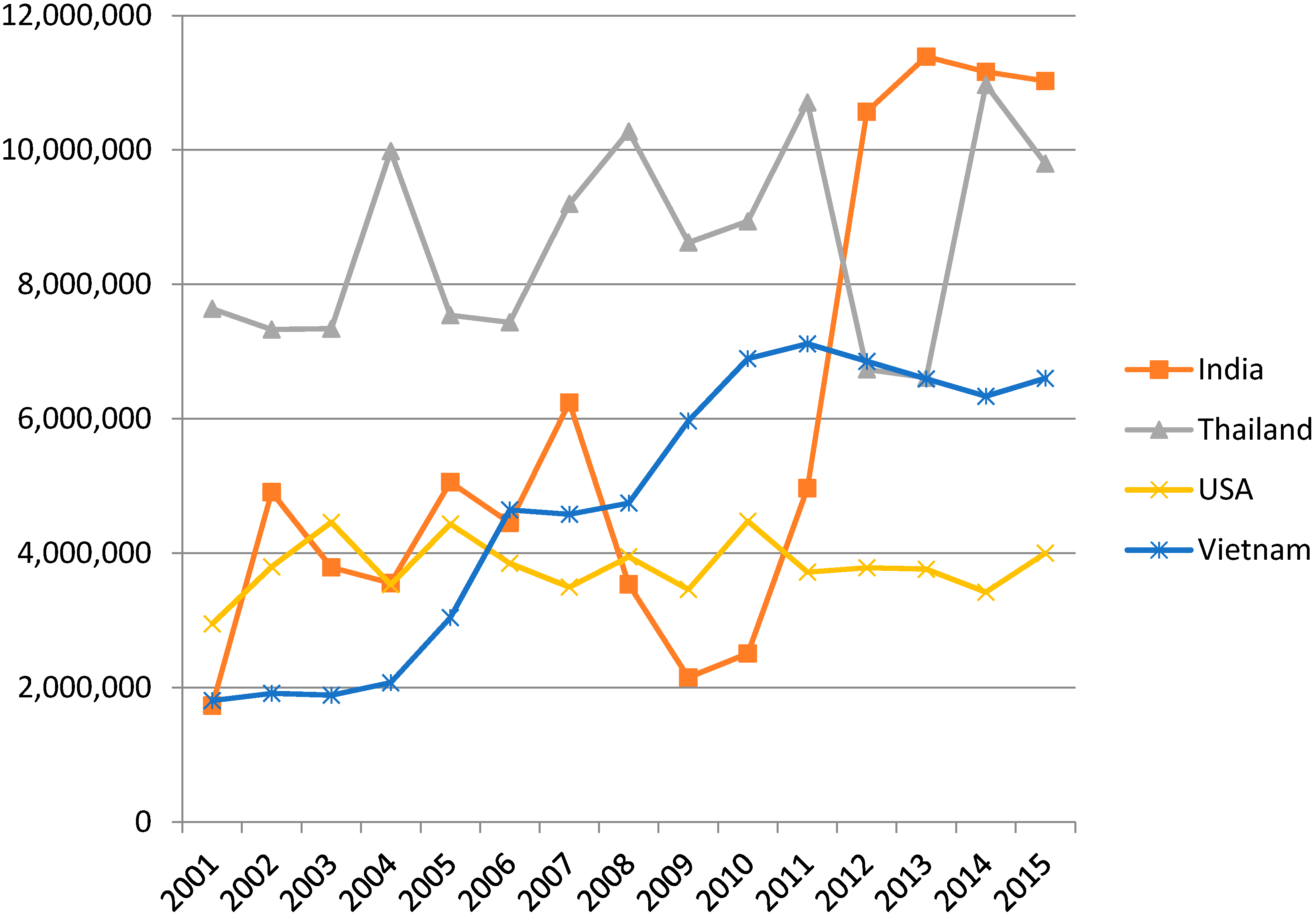
Challenges Facing the Thai Rice Economy

Thailand has long sustained its position as the world’s largest exporter for three decades, due primarily to the high quality of its long-grain milled rice, and the unique qualities of Thai Hom Mali rice (i.e., the Jasmine rice). However, Thailand’s competitive advantage has been steadily eroded in the face of fierce commodity price competition from other exporters. Figure 1 displays rice exports from the top four exporting countries, i.e., India, Thailand, USA and Vietnam. We see that India has beaten Thailand to become the largest exporter of rice in the world since 2012. Thailand rice exports reached 10.7 million tons in 2011, then dropped to 6.7 million tons in 2012 and 6.6 million tons in 2013 [5]. This was due to Thailand’s worst floods in half a century, and the-then government’s rice scheme that adversely impacted rice production and export.

In 2012, India lifted its ban on rice exports, and 10 million tons of Indian rice flooded the market. Global prices plummeted. Thus, the Thai rice scheme stockpiled 17–18 million tons of rice that could not be sold, at prices that covered production-only costs [6]. Some researchers have found that Thailand does not have the ability to influence the export price of rice. For example, John [7] found that the Thai domestic pricing programs do not heavily distort world rice prices. Mahanaseth and Tauer [8] tested for the existence and extent of market power in a range of major Thai rice export destinations, and found that Thailand’s ability to influence its export price is constrained by competition from Vietnam and India, especially for low-quality and generic rice varieties.

Thailand is also facing severe water shortage, an essential input in rice production. Rice production uses large amounts of water. For example, 1.432 L water is needed to produce 1 kg of rice in an irrigated lowland production system [9]. The water shortage in Thailand is caused by the low level of water in reservoirs and reduced rainfall capacity, which is an effect of extreme climatic conditions, such as El Nino phenomenon. Major rice fields have been severely damaged by drought. If there is less rainfall than predicted in the rainy season, billions of baht worth of damage in rice yield will reduce Thai economic growth by 0.4%. Although El Nino is a global phenomenon, global rice prices may increase only slightly as a result of a widespread fall in rice supply. Average rainfall in Thailand is 46% lower than normal, and water levels are at 45% of reservoir capacity. As a result, farm output has declined by 7–8% in 2015 and 2016, and farmers’ debt to agricultural income has risen to 100% due to the impact of drought [10].

The Thai agricultural sector is also experiencing labor shortage as farmers move into better-paid manufacturing and services sectors, and those who remained in farming are older. Average farm income is 14,211 baht per month, while the national average income is 21,566 baht per month, and the professional, technical, and administrative workers have the highest income, of approximately 51,866 baht [11].

As mentioned, aging of the farmers is another issue. According to government statistics, the average age of farmers jumped from 31 years in 1985 to 42 in 2010. Only 12% of the farmers were under 25, as compared to 34% in 1985 [11].

With respect to the use of chemicals, the government has encouraged the intensification of chemical fertilizers as the main approach to increase crop production. But increased fertilizer use did not see a corresponding increase in yield, which may have been be due to a lack of knowledge on the actual effectiveness of chemicals, resulting in technically inefficient use of chemicals in Thai agriculture [12].

In addition, technological constraints like low-yielding varieties are other major threats. In recent decades, Thai agriculture has shifted towards higher-value crops with increased mechanization, in order to remain competitive and raise farmers’ incomes. However, it has appeared to have little effect. We see that Thailand continues to lag behind its Asian neighbors on agricultural productivity, as shown in Figure 2. Rice yield is not stable, and has showed only a moderate level of increase over time. Price instability in the international rice market exerts a high level of influence on domestic rice production. For example, Jasmine rice accounts for approximately half of rice export incomes in Thailand—an important source of foreign currency reserves [13]. But the market value of Jasmine rice has fallen over a third since 2013, and is at a nine-year low [13]. Thus, the current government has proposed a 35.8 billion baht ($1.02 billion) loan scheme that is aimed at curbing an oversupply of Jasmine rice in the market, and stabilizing prices [14].

All of these factors may prompt Thai farmers to give up rice planting and engage in rubber and fruit tree plantations, fishery, and vegetable cultivation [15]. Therefore, Thailand urgently needs to increase productivity and efficiency in rice farming, in order to not only to be competitive in the rice export market, but also to sustain the nation’s food security and rural employment, and conserve culture and tradition, which is largely linked to the rice economy.

Given this backdrop, the aims of the present study are to: (a) measure the existing level of productivity and efficiency of rice farmers; (b) identify the determinants of inefficiency; and (c) estimate potential productivity increase and/or resource conservation, once inefficiency of rice farmers can be eliminated in Thailand.

We undertook this task by applying a Zero Inefficiency Stochastic Frontier Model (ZISFM) on a sample of 300 rice farmers from central-northern Thailand, which is the main rice growing area. The contributions of our study to the existing literature were two-fold: first, we used a ZISFM, a recently introduced but not commonly used method of efficiency estimation (discussed below). Second, we used the parameters of the estimated model to develop scenarios of potential production increase per unit of land and resource savings per unit of output in Thailand when technical inefficiency was eliminated, which is not commonly seen in the literature. Such scenarios will provide compelling evidence leading to the development of well-informed policies aimed at eliminating technical inefficiency to sustain agricultural growth.

There are two primary methods of efficiency measures, namely stochastic frontiers and data envelopment analysis (DEA), which involve econometric methods and mathematical programming, respectively. Stochastic frontier models make assumptions about the functional form of production or cost functions, and can deal effectively with the presence of noise in the data, whereas DEA models make no assumptions about the functional forms, but cannot deal effectively with measurement error [16]. Coelli [17] recommended the stochastic frontier method for use in most agricultural applications, and also pointed out that the stochastic frontier model has the added advantage of the ability to conduct statistical tests of hypotheses regarding the production structure and the degree of inefficiency. Therefore, the stochastic frontier model is more suitable than DEA in this study.

The Stochastic frontier model (SFM) is usually used to measure technical efficiency or inefficiency scores for each individual. It was proposed independently by Aigner et al. [18] and Meeusen and Broeck [19]. This method has been widely used in many research fields for technical efficiency analysis, particularly in agricultural economics. For example, Chen and Song [20] used the stochastic frontier model to examine technical efficiency and the technology gap in China’s agriculture. Rahman et al. [21] applied stochastic frontier model to model the technical efficiency of rice farmers in Bangladesh. Yang et al. [22] investigated the presence of production risk and technical inefficiency for a sample of rice farms in the Xiangyang City of China using a stochastic production frontier framework. Kim et al. [23] utilized the stochastic production frontier model to examine productivity of inputs for small and medium companies in Korea. Avea et al. [24] studied how NGOs and development agencies contribute to the sustainability of smallholder soybean farmers in northern Ghana by using a stochastic frontier approach.

However, the commonly used stochastic frontier approach mentioned above assumes that all individuals are inefficient. This is a strong assumption and potentially overstates inefficiency, or underestimates efficiency, and is susceptible to bias in drawing policy implication. Kumbhakar et al. [25] proposed ZISFM to relax this assumption. In this study, we applied the ZISFM to analyze technical efficiency and inefficiency. The ZISFM successfully allows fully efficient firms to be accounted for, from the onset of a stochastic frontier analysis, and the method can uncover anomalies that traditional methods wash away with the rigid assumption of inefficiency of all observations in the sample.

The rest of the paper is organized as follows: the methodology and the data are presented in Section 2, empirical results in Section 3; and the conclusion and policy recommendations in Section 4.

2. Methodology

2.1. The Zero Inefficiency Stochastic Frontier Model (ZISFM)

Following Kumbhakar et al. [25] and Tran and Tsionas [26], a ZISF production model for cross-sectional data was specified as

$$y_i=x_i^{\prime }\beta +v_i\mathrm{with}\mathrm{probability}p,$$

(1)

$$y_i=x_i^{\prime }\beta +v_i-u_i\mathrm{with}\mathrm{probability}1-p$$

where the error term in the SFM is defined as ${\epsilon }_i=v_i-u_i$, y_i, which represents the output of firm i, x_i denotes a $K\times 1$ vector whose values are functions of inputs and other explanatory variables, $\beta$ is the vector of parameters corresponding to explanatory variables, v_i is assumed to be i.i.d random errors and normal distribution with mean 0 and unknown variance ${\sigma }_v^2$, u_i are non-negative unobservable random variables following a half normal distribution with mean 0 and unknown variance ${\sigma }_u^2$, p is a function that represents the proportion of firms that are fully efficient, and p is specified as p = exp(γ)/[1 + exp(γ)].

The density function of ${\epsilon }_i$ is a mixture between a normally distributed random variable, and a convoluted density from a normal/half-normal SFM. The conditional probability density function of ${\epsilon }_i$ can be expressed as

$$f\left(\epsilon |x\right)=\left(\frac{p}{{\sigma }_v}\right)g\left(\frac{\epsilon }{{\sigma }_v}\right)+\left(1-p\right)[\frac{2}{\sigma }g(\frac{\epsilon }{\sigma })G(-\epsilon \frac{\lambda }{\sigma })]$$

(2)

where ${\sigma }^2={\sigma }_u^2+{\sigma }_v^2$, $\lambda ={\sigma }_u/{\sigma }_v$, g and G are normal probability density functions and normal cumulative distribution functions, respectively. Then, the conditional log-likelihood is given by

$$\log L={\displaystyle \sum }_{i=1}^n\log \left(f\left({\epsilon }_i\mid x_i\right)\right)={\displaystyle \sum }_{i=1}^n\log \left\{\left(\frac{p}{{\sigma }_v}\right)g\left(\frac{y-x^{\prime }\beta }{{\sigma }_{\upsilon }}\right)+\left(1-p\right)\left[\frac{2}{\sigma }g\left(\frac{y-x^{\prime }\beta }{\sigma }\right)\mathrm{G}\left(-\left(y-x^{\prime }\beta \right)\frac{\lambda }{\sigma }\right)\right]\right\}$$

(3)

We resort to a pseudo-likelihood ratio (PLR) to test full efficiency following Kumbhakar et al. [25]. The PLR test is defined as $\mathrm{PLR}=-2\left({\mathrm{L}}_{\mathrm{N}}-{\mathrm{L}}_{\mathrm{ZI}}\right)$, where L_N is the log-likelihood of the normal linear regression, L_ZI is the log-likelihood of the ZISFM. The PLR test has an asymptotic distribution which constitutes a 50:50 mixture of ${\mathsf{\chi }}_0^2$ and ${\mathsf{\chi }}_1^2$ distributions [27]. The null hypothesis is H₀: ${\sigma }_u=0$. Since we are focusing on the probability of being fully efficient, a rejection of the null hypothesis implies that fully efficient farms exist in correspondence with the proportion p. Kumbhakar et al. [25] provided asymptotic critical values, 1.642, 2.7043, 5.4133, for 90%, 95%, and 99% , respectively. However, we have to mention that PLR test is not perfect. For example, Rho and Schmidt [28], and Parmeter and Kumbhakar [29] found that p is not identified with incorrectly skewed OLS residuals. However, PLR is still the best compared with the Wald test, LM test, modified LM test, and Kuhn–Tucker test, and the PLR test is reasonable when λ is large (for details please see [28,29]).

2.2. Estimation of Farm-Specific Inefficiency and Technical Efficiency

The conditional density function of u given ε following Jondrow et al. [30] is 0 with probability $\pi \left(z_i\right)$ and $N_{+}\left({\mu }_{*},{\sigma }_{*}^2\right)$ with probability $1-\pi \left(z_i\right)$, where $N_{+}\left({\mu }_{*},{\sigma }_{*}^2\right)$ is expanded as follows:

$$f(u\mid \epsilon )=\frac{g\left(\left(u-{\mu }_{*}\right)/{\sigma }_{*}\right)}{{\sigma }_{*}G\left(-\epsilon \lambda /\sigma \right)},$$

(4)

where ${\mu }_{*}=-\epsilon {\sigma }_u^2/{\sigma }^2$ and ${\sigma }_{*}^2={\sigma }_u^2{\sigma }_v^2/{\sigma }^2$. Therefore, the conditional mean of u given $\epsilon =y-x^{\prime }\beta$, technical inefficiency, is expressed as

$${\rm E}\left(u\mid \epsilon \right)=\left(1-p\right)\frac{\sigma \lambda }{1+{\lambda }^2}\left[\frac{g\left(-\lambda \epsilon /\sigma \right)}{G\left(-\lambda \epsilon /\sigma \right)}-\frac{\lambda \epsilon }{\sigma }\right]$$

(5)

An estimated technical inefficiency can be obtained by replacing all unknown parameters in ZISFM and the estimated error term ${\widehat{\epsilon }}_i$. In addition, a flexible approach to measuring inefficiency can be constructed by using posterior estimate of probability that takes the form:

$$p_{\mathrm{i}}^{*}=\frac{{\widehat{p}}_i/{\widehat{\sigma }}_{v}g({\widehat{\epsilon }}_i/{\widehat{\sigma }}_v)}{{\widehat{p}}_i/{\widehat{\sigma }}_{v}g({\widehat{\epsilon }}_i/{\widehat{\sigma }}_v)+(1-{\widehat{p}}_i)(2/\widehat{\sigma })g({\widehat{\epsilon }}_i/\widehat{\sigma })G(-{\widehat{\epsilon }}_i{\widehat{\lambda }}_i/\widehat{\sigma })}$$

(6)

The posterior estimate of inefficiency is ${\tilde{u}}_i=\left(1-p_i^{*}\right){\widehat{u}}_i$, where ${\widehat{u}}_i$ is the estimated inefficiency from the ZISF. Thus, we call it posterior inefficiency. There are many studies considering technical efficiency scores, such as [31,32,33,34] etc. Battese and Coelli [35] observed that the difference between the two estimates reflects the inaccuracy of the approximation 1 − u_it to exp(−u_it). Therefore, we also constructed the technical efficiency in ZISFM, following Battese and Coelli [35]. The technical efficiency in ZISFM can be written as

$$E\left(\exp \left(-\left(1-p_i^{*}\right)U_i\right)\mid {{\rm E}}_i={\epsilon }_i\right)={{\displaystyle \int }}_0^{+\infty }\exp \left(-\left(1-p_i^{*}\right)u_i\right)f_{U_{i\mid E_{i={\epsilon }_i}}}\left(u_i\right)d{u}_i$$

$$=\left[\frac{1-G\left(\left(1-p_i^{*}\right){\sigma }_{*}-{\mu }_{*i}/{\sigma }_{*}\right)}{1-G\left(-u_{{*}_i}/{\sigma }_{*}\right)}\right]exp\left\{-\left(1-p_i^{*}\right){\mu }_{{*}_i}+\frac{1}{2}\left(1-p_i^{*}\right)²{\sigma }_{*}^2\right\}$$

(7)

We used the posterior odd ratio to censor our sample. The posterior odd ratio is defined as $R_i=p_i^{*}/\left(1-p_i^{*}\right)$. This ratio is greater than one for most of the censored (fully efficient) farmers. After we formally classified farmers into censored and non-censored groups, the censored SFM was constructed.

The prediction of the stochastic frontier output is important for farmers and policy makers. Based on Equations (1) and (7), the stochastic frontier output can be expressed as

$$Y_i^{*}=Y_i/T{E}_i=\frac{\exp \left(X_i\beta +v_i-u_i\right)}{\exp \left(u_i\right)}=\exp \left(X_i\beta +v_i\right)$$

(8)

Therefore, the averaged additional output, $\Delta$ can be directly calculated by using $1/N{\displaystyle \sum }_{i=1}^N(Y_i^{*}-Y_i)$. If the unit of output is ton/ha, the total additional output will be easy to compute by $\Delta$ multiplied by the total land area of rice grown.

In addition to being used to calculate technical efficiency and technical inefficiency, ZISFM and posterior ZISFM can be used to measure resource saving as well. According to the estimates of technical efficiency, the probability of full efficiency and the posterior odd ratios, we can identify efficient farms and inefficient farms. Thus, the sample is separated into two groups: inefficient group and efficient group. First, we calculated the input of actual production factors required to produce one ton of rice for efficient farmers and inefficient farmers, respectively. The input of actual production factors for efficient farmers and inefficient farmers, ${\dot{x}}_j$ and ${\ddot{x}}_j$, are given as follows

$$s_1=\frac{1}{N_1\times 1000}{{\displaystyle \sum }}_{i=1}^{N_1}{Y}_i{\dot{x}}_j=\frac{1}{s_1\times N_1}{{\displaystyle \sum }}_{i=1}^{N_1}{X}_{ij},$$

(9)

$$s_2=\frac{1}{N_2\times 1000}{{\displaystyle \sum }}_{i=1}^{N_2}{Y}_i{\ddot{x}}_j=\frac{1}{s_2\times N_2}{{\displaystyle \sum }}_{i=1}^{N_2}{X}_{ij},$$

(10)

respectively, where N₁ is the number of efficient farmers, N₂ is the number of inefficient farmers, j = 1, 2, …, j represents the number of production factors. Second, the resource saving of producing one ton of rice is defined as $R{S}_j={\ddot{x}}_j-{\dot{x}}_j$. Last, the total resource saving can be computed as

$$TR{S}_j=yield\times \left(1-p\right)\times R{S}_j$$

(11)

where yield is the annual rice production, p is the parameter in ZISFM.

The log likelihood function Equation (3) was computed using the BFGS algorithm in the maxLik package of R software. Some starting values were obtained from the conventional SFM in the frontier package in R software.

2.3. The Data

A total of 300 rice farmers from central-northern Thailand (Kamphaeng Phet province) constituted the sample population of the study. The data were collected during the year 2012. A random sampling procedure was employed. Details of output and input data were collected from these rice farmers, using face to face interviews conducted by graduate level research students of the Chiang Mai University, Chiang Mai, Thailand. Kamphaeng Phet province is one of the most important rice production areas in the central north of Thailand. There are 2.29 thousand km² for planting rice, which is 3% of total rice area in Thailand. Also, the Ping river and Bhumibol dam on the Ping river provide convenient conditions for planting rice. Farming is the most common economic activity for Thai workers in this area, because of the abundance of lowlands, which are most suitable for agriculture. The central region is often called the ‘rice bowl’ of Thailand, being the most fertile area of the country. This region also enjoys the highest per capita income in the country after Bangkok Metropolitan Area.

Rice can be planted in several ways, but most commonly, it is divided into two categories, direct seeding of rice (DSR) and transplanting seedlings. DSR can be done by hand or by machine. The farmers can be separated into three categories based on their planting patterns: transplanting seedlings, manual DSR, and mechanical DSR. Transplanting seedlings is the traditional planting pattern, while manual and mechanical DSR are popular planting pattern in recent times. DSR is an alternative option to for coping with the problems of water and labor scarcity associated with conventionally flooded rice. We have 100 observations for each seed planting category.

2.4. The Empirical Model

The empirical model is specified with a Translog stochastic production frontier function:

$$LnY={\alpha }_0+{{\displaystyle \sum }}_{j=1}^5{\alpha }_{j}Ln{X}_{ij}+{{\displaystyle \sum }}_{j=1}^5{{\displaystyle \sum }}_{k=1}^5{\beta }_{jk}\left(Ln{X}_{ij}Ln{X}_{ik}\right)+{{\displaystyle \sum }}_{m=1}^2{\phi }_m{R}_{im}+v_i-u_i,$$

(12)

$$u_i={{\displaystyle \sum }}_{d=1}^7{\delta }_d{Z}_{id}+e_i$$

(13)

where Y_i is the rice output; X_ij is the jth input for the ith farmer; R_im is the dummy variable for farms located in the plain land and farms located in slopes, v_i is the two sided random error, u_i is the one sided half-normal error, ln natural logarithm, e_i is the truncated random variable; α₀, α_j, β_j, ${\phi }_m$ and δ_d are the parameters to be estimated.

A total of five production inputs (X) and two regional dummies (R) were used in the production function, and four variables representing socio-economic characteristics of the farmer (Z) were included in the inefficiency effects model as predictors of technical inefficiency. The production inputs are: land (m²), labor (person days), material inputs (which includes inorganic fertilizers, pesticides, and seeds) (baht), mechanical power (baht), and irrigation (baht). The factors influencing technical inefficiencies were specified as: Educ1 = Dummy variable showing value of 1 if the farmer was at a primary education level, otherwise zero; Educ2 = Dummy variable showing value of 1 if the farmer was at a secondary education level, otherwise zero; Educ3 = Dummy variable showing value of 1 if the farmer was at college education level and above, otherwise zero; Share = The share of hired labor used in growing rice (proportion of total labor); Pattern1 = Dummy variable showing value of 1 if the farmer used manual DSR to plant rice; Pattern2 = Dummy variable showing a value of 1 if the farmer used mechanical DSR to plant rice; Pattern3 = Dummy variable showing value of 1 if the farmer used transplanting seedlings to plant rice.

3. Empirical Results

In this section, we report the parameter estimates and results of the technical inefficiency and technical efficiency analyses. Starting with the parameter estimates,

Table 1. Parameter estimates of the conventional Stochastic Frontier models (SFM) and Zero Inefficiency Stochastic Frontier models (ZISFM).

Parameters	Traditional SFM	ZISFM	Censored SFM
Production Frontier
Constant	10.3247 ***	10.3298 ***	10.3613 ***
	(0.1256)	(0.1263)	(0.0295)
ln Labor	0.0927 **	0.0813 *	0.1576 ***
	(0.0401)	(0.0451)	(0.0249)
ln Land	0.6835 ***	0.7096 ***	0.6376 ***
	(0.2125)	(0.2269)	(0.1071)
ln Input	0.2163	0.1965	0.2031
	(0.2047)	(0.2140)	(0.1301)
ln Mechanical power	0.0009	0.0048	0.0150
	(0.0336)	(0.0316)	(0.0214)
ln Irrigation	−0.0228	−0.0341	−0.0439 ***
	(0.0659)	(0.0654)	(0.0001)
Slope	0.0042	0.0037	−0.0044
	(0.0189)	(0.0157)	(0.0322)
Plain	0.0318	0.0274	0.0276
	(0.0307)	(0.0258)	(0.0323)
0.5 × (ln Labor)2	−0.6943 ***	−0.7098 ***	−0.6365 ***
	(0.0875)	(0.0803)	(0.0644)
0.5 × (ln Land)2	1.7191 ***	1.6421 ***	1.5963 ***
	(0.3579)	(0.3523)	(0.4124)
0.5 × (ln Input)2	−0.1523 **	−0.1566 **	−0.0408
	(0.0731)	(0.0668)	(0.1049)
0.5 × (ln Mechanical power)2	−0.0290	−0.0294	−0.0303
	(0.0232)	(0.0215)	(0.0256)
0.5 × (ln Irrigation)2	−0.0031	−0.0048	−0.0061 ***
	(0.0094)	(0.0094)	(0.0001)
ln Labor × ln Land	−0.4590 *	−0.4208 *	−0.4246 ***
	(0.2395)	(0.2277)	(0.1591)
ln Labor × ln Input	0.7230 ***	0.6824 ***	0.7195 ***
	(0.2531)	(0.2405)	(0.1632)
ln Labor × ln Mechanical power	0.0726 *	0.0766 *	0.0049
	(0.0420)	(0.0407)	(0.0479)
ln Labor × ln Irrigation	0.0031	0.0029	0.0065 ***
	(0.0021)	(0.0022)	(0.0019)
ln Land × ln Input	−0.8664 ***	−0.8213 ***	−0.8659 ***
	(0.1800)	(0.1787)	(0.2160)
ln Land × ln Mechanical power	−0.8412 ***	−0.8903 ***	0.4364
	(0.3207)	(0.2967)	(0.3203)
ln Land × ln Irrigation	−0.0231 *	−0.0210	−0.0203 **
	(0.0122)	(0.0138)	(0.0082)
ln Input × ln Mechanical Power	0.8722 ***	0.9255 ***	0.4608
	(0.3099)	(0.2879)	(0.3121)
ln Input × Ln irrigation	0.0202 *	0.0184	0.0136
	(0.0118)	(0.0130)	(0.0094)
ln Mechanical power × ln Irrigation	−0.0010	−0.0009	0.0004
	(0.0022)	(0.0021)	(0.0014)
Model diagnostics
p	---	0.1333 **	---
		(0.0599)
σ2	0.0202 ***	0.0195	0.0176
	(0.0033)
γ	0.9563 ***	0.9568	0.9992
	(0.0424)
σu	0.1388	0.1365 ***	0.1327 ***
		(0.0032)	(0.0035)
σv	0.0297	0.0290 ***	0.0037 ***
		(0.0015)	(0.0001)
λ	4.6806	4.7097	12.7535
PLR test	---	13.2333 ***	---
Inefficiency effect
Educ1	−0.0316	−0.0252	−0.0407 **
	(0.0227)	(0.0193)	(0.0177)
Educ2	−0.0381	−0.0312	0.0507 **
	(0.0250)	(0.0212)	(0.0212)
Educ3	−0.0689 ***	−0.0542 ***	−0.0981 ***
	(0.0236)	(0.0199)	(0.0213)
Share of hired labor	0.0111	0.0105	−0.0131
	(0.0166)	(0.0142)	(0.0189)
Planting pattern1	0.1959 ***	0.1568 ***	0.2164 ***
	(0.0229)	(0.0195)	(0.0182)
Planting pattern2	0.1299 ***	0.0976 ***	0.1502 ***
	(0.0233)	(0.0198)	(0.0189)
Planting pattern3	0.1012 ***	0.0763 ***	0.1157 ***
	(0.0225)	(0.0191)	(0.0173)
R2	0.7696	0.7412	0.7622

Note: *** = significant at 1% level (p < 0.01); ** = significant at 5% level (p < 0.05); * = significant at 10% level (p < 0.10).

shows parameter estimates of the traditional SFM, the ZISFM and the censored SFM. It is clear that the PLR (Posterior Likelihood Ratio) test in the ZISFM is statistically significant at 1% level, which means that there were some fully efficient farmers present in the total sample. The probability of efficiency from the ZISFM was p = 0.1333, and statistically significant at 1% level, which also showed that there are two classes, fully efficient and inefficient farmers in this sample. The number of the cut-off sample was 22, and it accounted for about 7% of the total sample. Thus, we classified the farmers into censored and non-censored groups, and estimated censored SFM and censored ZISFM. The probability of efficiency from the censored ZISFM was 0.08, which was close to the proportion of censored sample and was expected.

In the traditional SFM, the variance of u was bigger than the other two models because the probability of efficiency pulled down the variance of inefficiency. On the other hand, the variance of v in the censored SFM was much lower than the traditional SFM and ZISFM, which implied that the censored SFM fit very well. Following Battese and Coelli [36], the parameters (${\sigma }_u$, ${\sigma }_v$) can be transformed to (λ, ${\sigma }^2$) with $\lambda ={\sigma }_u/{\sigma }_v$ and ${\sigma }^2={\sigma }_u^2+{\sigma }_v^2$. The larger λ, the greater the inefficiency component in the model. We also measured the global inefficiency by $\gamma ={\sigma }_u^2/{\sigma }^2$. The values of λ and γ revealed whether inefficiency played an important role in the composite error term [37]. The estimate of λ in the censored SFM was the greatest, as expected. The estimates of γ in three models were over 0.95, and were statistically significant at the 1% level. This indicated that farm productivity differentials predominantly related to variations in management.

In the production frontier section, the coefficients of land and labor had positive signs as expected, and were also statistically significant. All of the input variables were mean-corrected $\left(X_{ik}-{\overline{X}}_k\right)$ so that their averages were zero. This approach enabled the coefficients on the first-order terms to be read directly as production elasticities for the individual inputs at the mean input values (see [33,38]). In the ZISFM, land had the highest elasticity value of 0.70, implying that a 1% increase in land area allocated to rice will increase production by 0.70%. This is not surprising and is similar to the results of Rahman et al. [33] and Sriboonchitta et al. [34]. The estimated returns to scale parameters, computed as the sum of estimated output elasticities of all inputs at their mean values, were 1.0066 for the traditional SFM, 0.9892 for the ZISFM, and 0.9926 for the censored SFM. These estimates reflected the fact that there are no scale diseconomies on the frontier. It also illustrated that the Thai farmers may increase their rice production by improving technical efficiency rather than by increasing production scale.

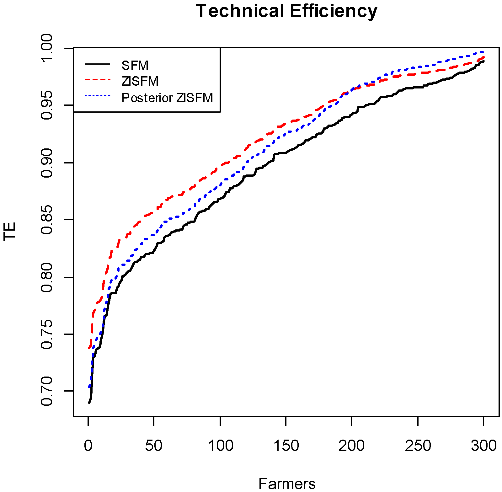
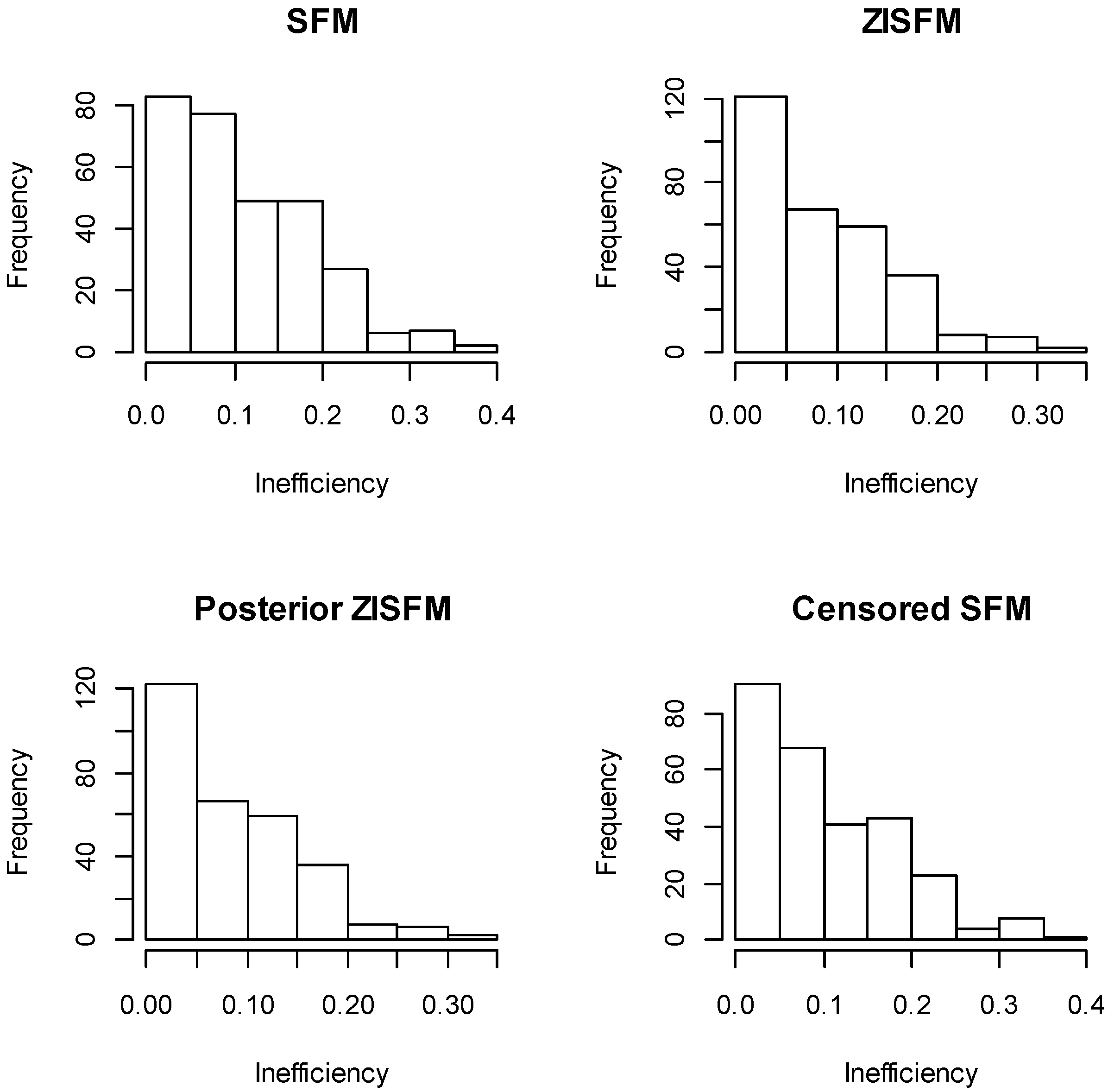
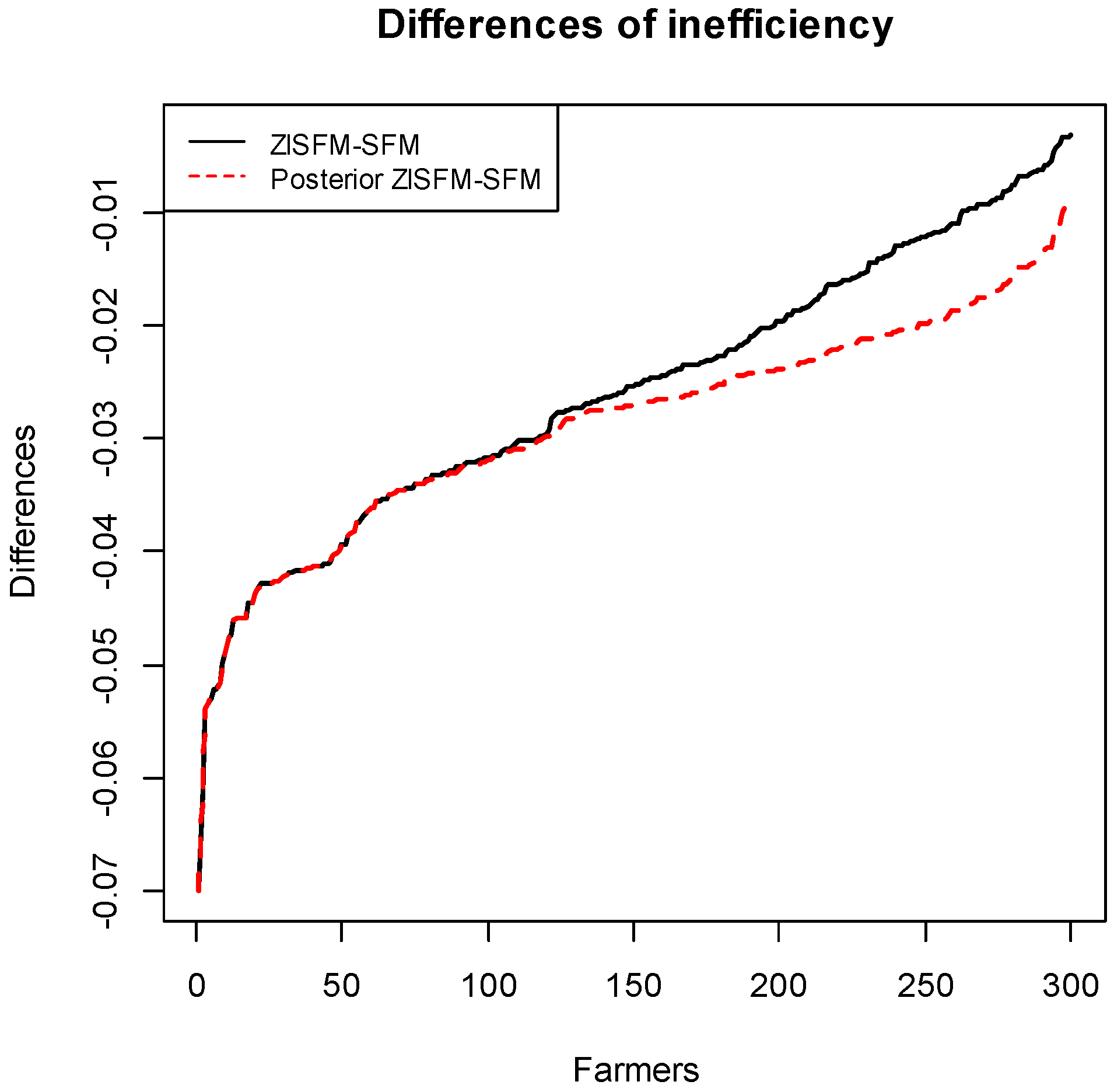
3.1. Technical Efficiency Distribution and Their Determinants

The lower part of Table 1 shows the parameter estimates of the technical inefficiency function. Since we used dummy variables for education and planting technology, we did not specify the intercept/constant term in the inefficiency function, to avoid collinearity. We found that the parameter estimates of the college education dummy variable carried a negative sign and was statistically significant at the 1% level in all three models. This result very clearly demonstrates that farmers’ education emerges as an important factor in enhancing technical efficiency. In the censored SFM, the parameter estimate of the college education dummy variable was much smaller than the other two models, which implies that education is more important for inefficient farmers. Asadullah and Rahman [39] also noted that education has a significantly positive influence on rice production efficiency in Bangladesh. Educated farmers usually have better access to information about prices, and the state of technology and its use [39]. Better-educated people also have a higher tendency to adopt and use modern inputs more optimally and efficiently. It is more likely that educated farmers are more perceptive to expert advice on agricultural production practices [21,40,41].

The parameter estimates for manually seed sowing, mechanical sowing, and transplanting seedlings had a positive effect on technical inefficiency, whereas the parameter estimate of the manual DSR was the largest, followed by mechanical DSR, and transplanting seedlings. The implication of this result is that farmers who are transplanting seedlings are relatively more technically efficient, while manual DSR is not a good planting technology, in Kamphaeng Phet province, Thailand. The reason for this relationship may be due to Thailand’s situation, where the farmers do not have sufficient technical knowledge about the use of modern planting techniques. Pandey et al. [42] also showed that the yield of DSR under farmers’ field conditions tended to be lower than that of transplanted rice. Poor and uneven establishment, and inadequate weed control were the major reasons for its poor performance. Also, the traditional technique, transplanting seedlings, has generally been well mastered by the farmers over time.

Figure 3 displays the cumulative technical inefficiency distribution based on the three methods. The SFM overestimated the technical inefficiency scores compared to the ZISFM, which was expected. The technical inefficiency scores from the posterior ZISFM and the ZISFM did not show much difference between each other. Figure 4 displays the technical efficiency distribution from the three models. The SFM technical efficiency scores were the exact opposite of inefficiency in Figure 3. Thus it can be seen that the ZISFM is useful for amending technical efficiency or inefficiency scores, by relaxing the assumption of full inefficiency. We find that all the farmers have a relatively high technical efficiency, between 0.7 and 1.

Figure 5 and Figure 6 present histograms of technical inefficiency and efficiency distributions for the sampled farmers, respectively. As previously seen, the technical inefficiency and efficiency distributions reflected consistent results. About half of the farmers had high technical efficiency, or lower inefficiency. Figure 7 and Figure 8 show the differences of technical inefficiency and efficiency between ZISFM and traditional SFM, and between posterior ZISFM and traditional SFM, respectively. As previously shown, the traditional SFM overestimated farmers’ technical inefficiency, or underestimated farmers’ technical efficiency.

We present minimum values, maximum values, and the quartiles, as well as mean and standard deviation of farmers’ technical inefficiency and efficiency in

Table 2. Summary of technical inefficiencies and efficiencies.

Inefficiency	Min	Q25	Median	Mean	Q75	Max	SD
SFM	0.0116	0.0439	0.0963	0.1121	0.1665	0.3709	0.0775
ZISFM	0.0084	0.0282	0.0673	0.0864	0.1331	0.3045	0.0657
Posterior ZISFM	0.0024	0.0207	0.0667	0.0835	0.1331	0.3045	0.0684
Censored SFM	0.0008	0.0597	0.0926	0.1188	0.1746	0.3757	0.0827
Technical Efficiency	Min	Q25	Median	Mean	Q75	Max	SD
SFM	0.6904	0.847	0.9086	0.8969	0.9574	0.9885	0.0673
ZISFM	0.7377	0.8756	0.9352	0.9194	0.9724	0.9917	0.0586
Posterior ZISFM	0.704	0.8579	0.9263	0.9112	0.9765	0.9972	0.0695
Censored SFM	0.6868	0.8398	0.9115	0.8910	0.9421	0.9991	0.06957

. As expected, the traditional SFM overestimated inefficiency in each quartile compared with the ZISFM and the posterior ZISFM. This result was consistent with Kumbhakar et al. [25]. However, our censored SFM conditional mean estimates of inefficiency were higher than the traditional SFM conditional mean estimates. The technical efficiency also showed similar results to technical inefficiency. These results once again suggest that ZISFM and posterior ZISFM should be used to estimate inefficiency or efficiency behavior instead of traditional SFM. According to the summary statistics of technical efficiency, we saw that more than half of the farmers operated at a relatively high level of technical efficiency—beyond 0.9. These results were consistent with the findings in Figure 6.

Table 3. Top five and bottom five technical efficiency scores of the individual farmers based on SFM, ZISFM, and posterior ZISFM.

Rank	SFM	TE	ZISFM	TE	Posterior ZISFM	TE
	Farmer ID		Farmer ID		Farmer ID
1	38	0.9885	38	0.9917	38	0.9972
2	69	0.9875	69	0.9908	69	0.9967
3	58	0.9874	58	0.9907	58	0.9966
4	70	0.9867	70	0.9900	70	0.9961
5	34	0.9851	68	0.9893	68	0.9955
…	…	…	…	…	…	…
296	195	0.7315	195	0.7717	195	0.7415
297	173	0.7291	173	0.7681	173	0.7376
298	185	0.7137	185	0.7514	185	0.7191
299	178	0.6941	42	0.7403	42	0.7068
300	42	0.6904	178	0.7377	178	0.7040

displays the top five and bottom five technical efficiency scores of individual farmers based on the SFM, ZISFM, and posterior ZISFM. We found that the ZISFM and the posterior ZISFM gave consistent ranks in the top five and bottom five technical efficiency scores, thereby confirming the trends shown in Figure 3 and Figure 4. Moreover, most of the farmers who practiced manual DSR scored high inefficiency or low technical efficiency, whereas farmers who transplanted seedlings scored high efficiency or low inefficiency levels. This was consistent with the results of the parameter estimates of technical inefficiency function.

3.2. Scenarios of Potential Production Increase and Resource Conservation

Table 4. Prediction of stochastic frontier output and total additional output in Thailand.

Total Sample	ZISFM (ton/ha)	Posterior ZISFM (ton/ha)
Stochastic frontier output	7.7390	7.8146
Actual output	7.1234	7.1234
Additional output	0.6155	0.6912
Increasing rate	8.64%	9.7%
Total additional output	5,663,217 tons	6,359,295 tons
Planting Pattern 1	ZISFM	Posterior ZISFM
Stochastic frontier output	7.3006	7.4450
Actual output	6.3890	6.3890
Additional output	0.9115	1.0560
Increasing rate	14.27%	16.53%
Total additional output	2,795,414 tons	3,238,462 tons
Planting Pattern 2	ZISFM	Posterior ZISFM
Stochastic frontier output	7.8210	7.8810
Actual output	7.2843	7.2843
Additional output	0.5366	0.5966
Increasing rate	7.37%	8.19%
Total additional output	1,645,684 tons	1,829,760 tons
Planting Pattern 3	ZISFM	Posterior ZISFM
Stochastic frontier output	8.0953	8.1178
Actual output	7.6968	7.6968
Additional output	0.3985	0.4210
Increasing rate	5.18%	5.47%
Total additional output	1,222,120 tons	1,291,073 tons

reports on the prediction of stochastic frontier output and total additional output that can be produced in Thailand based on the results of ZISFM and posterior ZISFM. Total rice output could be increased by 8.64% on average, based on the results of ZISFM. Farmers practicing manual DSR have the biggest room to enhance rice production, followed by those who practice mechanical DSR, followed by farmers transplanting seedlings. Thailand has approximately 9.2 million hectares of rice growing area [43]. Therefore, we estimated the potential additional output that can be obtained by eliminating technical inefficiency (Table 4). The total additional output was estimated at approximately 5.6 million tons and 6.4 million tons, corresponding to the results of ZISFM and posterior ZISFM, respectively. The potential for increasing the total rice production by practicing manual DSR was high because these farmers were the least efficient, which implies that the technological knowhow of manual DSR must be improved. Although these production figures were substantial, they were expected.

Table 5. Resource savings in rice production of one ton, and total resource savings of Thailand in 2016, based on ZISFM and posterior ZISFM.

ZISFM	Labor (Person Days)	Land (m2)	Material Inputs (Baht)	Mechanical Power (Baht)
Efficient farmers	0.5671	1267.52	3570.936	3662.076
(N1 = 40, 13%)
Inefficient farmers	0.7040	1439.52	4033.14	4009.931
(N2 = 260, 87%)
Resource saving per ton	0.1369	172.00	462.2044	347.8546
Resource saving %	19.44%	11.95%	11.46%	8.67%
Total saving in Thailand	2,978,334	3,741,513,600	10,052,945,485	7,565,837,280
Posterior ZISFM
Efficient farmers	0.5637	1236.00	3390.375	3452.244
(N1 = 22, 7% of total)
Inefficient farmers	0.6939	1429.44	4014.93	4003.066
(N2 = 278, 93% of total)
Resource saving per ton	0.1301	193.44	624.5557	550.8216
Resource saving %	18.75%	13.53%	15.55%	13.76%
Total saving in Thailand	3,026,106	4,499,564,800	14,520,920,054	12,806,601,503

presents potential resource savings in producing one ton of rice, and the total resource savings of Thailand for the year 2016 based on the results of ZISFM and posterior ZISFM. Webb [44] showed that Thailand aimed for 25 million tons of rice output in 2017. Based on ZISFM results, 19.44%, 11.95%, 11.46% and 8.67% of labor, land, material inputs and mechanical power respectively could be saved to produce one ton of rice if technical inefficiency is eliminated. This translates into a resource conservation of 2.97 million of labor days, 3.74 thousand km² of land area, 10.05 billion baht of material input and 7.57 billion baht of mechanical power costs for one year in Thailand, which is substantial. The corresponding figures are similar and/or higher based on the results from posterior ZISFM (Table 5). Such prediction of scenarios provides compelling evidence to undertake policy decisions aimed at eliminating technical inefficiency in agriculture.

4. Conclusions

The main objectives of this paper were to estimate technical efficiency, and their determinants on rice farmers from central-northern Thailand, and then to develop scenarios of potential production increase and resource savings in rice production for Thailand. We did this by applying a recently introduced and less commonly used ZISFM, which allowed us to determine fully efficient farmers from the sample, and then estimate inefficiency of inefficient farmers. This addressed the potential overstatement of inefficiency arising from applying conventional SFM, which assumes that all farmers are inefficient.

Results revealed that 13% of the farmers were fully efficient in the sample, thereby justifying the use of ZISFM approach in our study. Land was the most important driver of rice production, followed by labor, which had a relatively smaller impact on rice productivity. Although the mean level of technical efficiency of the rice farmers was estimated at 91%, we still can improve technical efficiency in order for sustained agriculture to continue. Amongst the determinants of technical inefficiency, results revealed that the college-level education had the highest impact on improving efficiency. Seed planting technology also significantly influenced technical inefficiency. Farmers who transplanted seedlings were relatively more technically efficient compared to those who practiced manual DSR and mechanical DSR. The technical efficiency level of manual DSR was the lowest and was evaluated as not a good planting technology. Use of DSR is still a new experience for farmers who have been practicing conventional methods of sowing for centuries. Also, the traditional technique, transplanting seedlings, is well mastered by the farmers.

Finally, our calculations showed that elimination of technical inefficiency could potentially generate an additional rice output of 5.68–6.35 million tons. Also, elimination of technical inefficiency could potentially conserve 2.9–3.0 million person days of labor input, 3.7–4.5 thousand km² of land area, 10.05–14.52 billion baht of material input and 7.56–12.81 billion baht of mechanical power costs, at the current level of annual rice production in Thailand; these are substantial savings.

The following policy implications can be drawn from the results of this study. Investments in education targeted for farmers will significantly improve technical efficiency. Although all categories of education have significant influence, the impact is highest for farmers attaining tertiary education; this requires policies that enable the promotion of higher levels of education for farmers. Next, the government should provide support for the introduction of advanced technology for DSR. DSR technology is practiced successfully in many parts of the world, such as China, Australia, Malaysia, the USA, and Sri Lanka [45]. Many researchers believe that DSR technology can improve yields, with less water and labor requirements. However, our results showed that this technology did not perform well in Thailand. Thus, we suggest that the government acquires the relevant knowledge and expertise from successful countries, by dispatching training programs for agricultural technicians and/or representative model farmers, on the use of modern planting technologies, and the acquisition of advanced equipment. Along with the aging Thai population, and water resource shortages, DSR is becoming increasingly important as a sustainable technology to replace traditional transplanting technology, although the latter is currently more efficient.

References

1. Ajewole, O.C.; Folayan, J.A. Stochastic frontier analysis of technical efficiency in dry season leaf vegetable production among smallholders in Ekiti state, Nigeria. Agric. J. 2008, 3, 252–257. [Google Scholar]
2. Bravo-Ureta, B.E.; Rieger, L. Dairy Farm Efficiency Measurement Using Stochastic Frontiers and Neoclassical Duality. Am. J. Agric. Econ. 1991, 73, 421–428. [Google Scholar] [CrossRef]
3. Afriat, S.N. Efficiency estimation of production functions. Int. Econ. Rev. 1972, 13, 568–598. [Google Scholar] [CrossRef]
4. Mishra, A.; Kumar, P.; Noble, A. Assessing the potential of SRI management principles and the FFS approach in Northeast Thailand for sustainable rice intensification in the context of climate change. Int. J. Agric. Sustain. 2013, 11, 4–22. [Google Scholar] [CrossRef]
5. Petchseechoung, W. Rice Industry. Thailand Industry Outlook; Krungsri Research: Bangkok, Thailand, 2016. [Google Scholar]
6. Arunmas, P.; Ruangdit, P. US Report Puts Thai Rice Edge in Doubt; Bangkok Post: Bangkok, Thailand, 2012. [Google Scholar]
7. John, A. Price Relations between Export and Domestic Rice Markets in Thailand. Food Policy 2013, 42, 48–57. [Google Scholar] [CrossRef]
8. Mahanaseth, I.; Tauer, L.W. Thailand’s Market Power in Its Rice Export Markets. J. Agric. Food Ind. Organ. 2014, 12, 109–120. [Google Scholar] [CrossRef]
9. IRRI. How to Manage Water? Rice Knowledge Bank, IRRI: Los Banos, The Philippines, 2002; Available online: http://www.knowledgebank.irri.org/step-by-step-production/growth/water-management (accessed on 20 March 2017).
10. Thaiturapaisan, T. Drought, a Worrying Situation for Thai Agriculture. 2015. Available online: https://www.scbeic.com/en/detail/product/1429 (accessed on 9 March 2017).
11. OECD. Economic Outlook for Southeast Asia, China and India 2014: Beyond the Middle-Income Trap. 2013. Available online: http://dx.doi.org/10.1787/saeo-2014-en (accessed on 14 March 2017).
12. Tirado, R.; Englande, A.J.; Promakasikorn, L; Novotny, V. Use of Agrochemicals in Thailand and Its Consequences for the Environment. Greenpeace Research Laboratories Technical Note. 2008. Available online: http://www.greenpeace.to/publications/GPSEA_agrochemical-use-in-thailand.pdf (accessed on 3 March 2017).
13. Franco, N. Thailand’s Rice Industry is in Crisis during a Politically Sensitive Period. 2016. Available online: https://www.linkedin.com/pulse/rice-market-news-17112016-negri-franco?articleId=8612683279200132720 (accessed on 17 March 2017).
14. Hariraksapitak, P.; Tanakasempipat, P. Thailand Offers $1 Billion Loan to Struggling Jasmine Rice Farmers; Thomson Reuters: New York, NY, USA, 2016. [Google Scholar]
15. Blake, C.; Suwannakij, S. Thai Junta Flip-Flop on Populism Too Late for Suffering Farmers. 2016. Available online: https://www.bloomberg.com/news/articles/2016-11-22/thai-junta-flip-flop-on-populism-too-late-for-suffering-farmers (accessed on 12 March 2017).
16. Tsionas, E.G. Combining DEA and stochastic frontier models: An empirical Bayes approach. Eur. J. Oper. Res. 2003, 147, 499–510. [Google Scholar] [CrossRef]
17. Coelli, T.J. Recent Development in Frontier Modeling and Efficiency Measurement. Aust. J. Agric. Econ. 1995, 39, 219–245. [Google Scholar] [CrossRef]
18. Aigner, D.J.; Lovell, C.A.K.; Schmidt, P. Formulation and estimation of Stochastic Frontier Production function models. J. Econ. 1977, 6, 21–37. [Google Scholar] [CrossRef]
19. Meeusen, W.; Broeck, V.D. Efficiency estimation from Cobb-Douglas production function with composed error. Int. Econ. Rev. 1977, 18, 435–455. [Google Scholar] [CrossRef]
20. Chen, Z.; Song, S. Efficiency and technology gap in China’s agriculture: A regional meta-frontier analysis. China Econ. Rev. 2008, 19, 287–296. [Google Scholar] [CrossRef]
21. Rahman, K.M.M.; Mia, M.I.A.; Bhuiyan, M.K.J. A Stochastic Frontier Approach to Model Technical Efficiency of Rice Farmers in Bangladesh: An Empirical Analysis. Agriculturists 2012, 10, 9–19. [Google Scholar] [CrossRef]
22. Yang, Z.; Mugera, A.W.; Zhang, F. Investigating Yield Variability and Inefficiency in Rice Production: A Case Study in Central China. Sustainability 2016, 8, 787. [Google Scholar] [CrossRef]
23. Kim, D.H.; Sambou, M.O.; Jung, M.S. Does Technology Transfer Help Small and Medium Companies? Empirical Evidence from Korea. Sustainability 2016, 8, 1119. [Google Scholar] [CrossRef]
24. Avea, A.D.; Zhu, J.; Tian, X.; Baležentis, T.; Li, T.; Rickaille, M.; Funsani, W. Do NGOs and Development Agencies Contribute to Sustainability of Smallholder Soybean Farmers in Northern Ghana—A Stochastic Production Frontier Approach. Sustainability 2016, 8, 465. [Google Scholar] [CrossRef]
25. Kumbhakar, S.C.; Parmeter, C.F.; Tsionas, E.G. A zero-inefficiency stochastic frontier model. J. Econ. 2013, 172, 66–76. [Google Scholar] [CrossRef]
26. Tran, K.C.; Tsionas, M.G. Zero inefficiency stochastic frontier models with varying mixing proportion: A semiparametric approach. Eur. J. Oper. Res. 2016, 249, 1113–1123. [Google Scholar] [CrossRef]
27. Coelli, T.J. Estimators and hypothesis tests for a stochastic frontier function: A Monte Carlo analysis. J. Product. Anal. 1995a, 6, 247–268. [Google Scholar] [CrossRef]
28. Rho, S.; Schmidt, P. Are all firms inefficient? J. Product. Anal. 2015, 43, 327–349. [Google Scholar] [CrossRef]
29. Parmeter, C.F.; Kumbhakar, S.C. Efficiency analysis: A primer on recent advances. Found. Trends Econ. 2014, 7, 191–385. [Google Scholar] [CrossRef]
30. Jondrow, J.; Lovell, C.A.K.; Materov, I.S.; Schmidt, P. On the estimation of technical inefficiency in the stochastic frontier production function model. J. Econ. 1982, 19, 233–238. [Google Scholar] [CrossRef]
31. Greene, W.H. A stochastic frontier model with correction for sample selection. J. Product. Anal. 2010, 34, 15–24. [Google Scholar] [CrossRef]
32. Rahman, S.; Rahman, M. Impact of land fragmentation and resource ownership on productivity and efficiency: The case of rice producers in Bangladesh. Land Use Policy 2009a, 26, 95–103. [Google Scholar] [CrossRef]
33. Rahman, S.; Wiboonpongse, A.; Sriboonchitta, S.; Chaovanapoonphol, Y. Production efficiency of Jasmine rice farmers in northern and northeastern Thailand. J. Agric. Econ. 2009b, 60, 419–435. [Google Scholar] [CrossRef]
34. Sriboonchitta, S.; Liu, J.; Wiboonpongse, A.; Denoeux, T. A double-copula stochastic frontier model with dependent error components and correction for sample selection. Int. J. Approx. Reason. 2017, 80, 174–184. [Google Scholar] [CrossRef]
35. Battese, G.; Coelli, T. A model for technical inefficiency effects in a stochastic frontier production function for panel data. Empir. Econ. 1995, 20, 325–332. [Google Scholar] [CrossRef]
36. Battese, G.E.; Coelli, T.J. Frontier production functions, technical efficiency and panel data: With application to paddy farmers in India. J. Product. Anal. 1992, 3, 153–169. [Google Scholar] [CrossRef]
37. Greene, W. Distinguishing between heterogeneity and inefficiency: Stochastic frontier analysis of the World Health Organization’s panel data on national health care systems. Health Econ. 2004, 13, 959–980. [Google Scholar] [CrossRef] [PubMed]
38. Asante, B.O.; Villano, R.A.; Battese, G.E. The effect of the adoption of yam minisett technology on the technical efficiency of yam farmers in the forest-savanna transition zone of Ghana. Afr. J. Agric. Resour. Econ. 2014, 9, 75–90. [Google Scholar]
39. Asadullah, M.N.; Rahman, S. Farm productivity and efficiency in rural Bangladesh: The role of education revisited. Appl. Econ. 2009, 41, 17–33. [Google Scholar] [CrossRef]
40. Chen, A.Z.; Wallace, E.H.; Scott, R. Technical Efficiency of Chinese Grain Production: A Stochastic Production Frontier Approach. In Proceedings of the American Agricultural Economics Association Annual Meeting, Montreal, QC, Canada, 27 July 2003. [Google Scholar]
41. Ahmad, M.; Chaudhry, G.M.; Iqbal, M. Wheat productivity, efficiency, and Sustainability: A stochastic production frontier analysis. Pak. Dev. Rev. 2002, 41, 643–663. [Google Scholar]
42. Pandey, S.; Mortimer, M.; Wade, L.; Tuong, T.P.; Lopez, K.; Hardy, B. (Eds.) Direct seeding: Research issues and opportunities. In Proceedings of the International Workshop on Direct Seeding in Asian Rice Systems: Strategic Research Issues and Opportunities, Bangko, Thailand, 25–28 January 2000; International Rice Research Institute: Los Baños, Philippines, 2002. [Google Scholar]
43. Nirmal, G. Thailand to Set Aside More Land for Farming; It Plans to Increase Rice Production and Stop Conversion of Agricultural Land; Straits Times: Singapore, 2008. [Google Scholar]
44. Webb, S. Thailand Aims for 25 mln T Rice Paddy Output 2016–17, down on yr; Reuters Africa: Kenya, Africa, 2016. [Google Scholar]
45. Ali, A.; Erenstein, O.; Rahut, D.B. Impact of direct rice sowing technology on rice producers’ earnings: Empirical evidence from Pakistan. Dev. Stud. Res. 2014, 1, 244–254. [Google Scholar] [CrossRef]
Figure 1. Rice exports of India, Thailand, US and Vietnam from 2001 to 2015 (metric tons). Source: Adapted from U.S. Department of Agriculture.
Sustainability 09 00770 g001
Figure 2. Rice yield (kg/ha) in Thailand and other Asian countries, 1980–2011. Source: Adapted from FAOSTAT.
Sustainability 09 00770 g002
Figure 3. Cumulative technical inefficiency distribution based on three methods.
Sustainability 09 00770 g003
Figure 4. Cumulative technical efficiency distribution based on three methods.
Sustainability 09 00770 g004
Figure 5. Histograms of inefficiency distribution for the Thai farmers.
Sustainability 09 00770 g005
Figure 6. Histograms of technical efficiency distribution for the Thai farmers.
Sustainability 09 00770 g006
Figure 7. The differences of inefficiency between the ZISFM and the traditional SFM, between the posterior ZISFM and the traditional SFM.
Sustainability 09 00770 g007
Figure 8. The differences of efficiency between the ZISFM and the traditional SFM, between the posterior ZISFM and the traditional SFM.
Sustainability 09 00770 g008