
A Comparison between Spatial Econometric Models and Random Forest for Modeling Fire Occurrence


1
State Key Laboratory of Fire Science, University of Science and Technology of China, Hefei 230026, China
2
Department of Geography and Geographic Information Science, University of Illinois at Urbana-Champaign, Champaign, IL 61820, USA
3
Department of Human Geography and Spatial Planning, Faculty of Geosciences, Utrecht University, P.O. Box 80125, 3508 TC Utrecht, The Netherlands
*
Author to whom correspondence should be addressed.
Sustainability 2017, 9(5), 819; https://doi.org/10.3390/su9050819
Submission received: 18 February 2017
/
Revised: 19 April 2017
/
Accepted: 11 May 2017
/
Published: 14 May 2017
Abstract
:Fire occurrence, which is examined in terms of fire density (number of fire/km2) in this paper, has a close correlation with multiple spatiotemporal factors that include environmental, physical, and other socioeconomic predictors. Spatial autocorrelation exists widely and should be considered seriously for modeling the occurrence of fire in urban areas. Therefore, spatial econometric models (SE) were employed for modeling fire occurrence accordingly. Moreover, Random Forest (RF), which can manage the nonlinear correlation between predictors and shows steady predictive ability, was adopted. The performance of RF and SE models is discussed. Based on historical fire records of Hefei City as a case study in China, the results indicate that SE models have better predictive ability and among which the spatial autocorrelation model (SAC) is the best. Road density influences fire occurrence the most for SAC, while network distance to fire stations is the most important predictor for RF; they are selected in both models. Semivariograms are employed to explore their abilities to explain the spatial structure of fire occurrence, and the result shows that SAC works much better than RF. We give a further explanation for the generation of residuals between fire density and the common predictors in both models. Therefore, decision makers can make use of our conclusions to manage fire safety at the city scale.
1. Introduction
Fire is a widespread phenomenon in modern life. In China in 2015, 1742 people were killed in fires, with an economic loss of nearly $0.6 billion [1]. The severe threats for human beings caused by fire make people aware of the necessity of predicting fire risk, and we should adopt efficient measures to prevent the occurrence of fire. However, how fire occurs and spreads is highly complex and it is still difficult to explain the reasons and predict future incidents. Fire is similar to other natural and human disasters that are imbued with uncertainty and occur in dynamic systems with biologically diverse and complicated structures [2]. Using temporal and spatial datasets, along with historical datasets of fire ignition, it is possible to build valid and meaningful models for explaining fire occurrence; therefore, we can adopt these results to benefit the management of fire safety, from which we could assess the conditions of fire occurrence from a quantitative viewpoint.
According to previous studies, many of which were done in forest regions, human-related predictors are critical for explaining fire occurrence on the large scales, such as in Europe and China [2,3,4,5,6]. However, few studies were done at the city scale to explain and predict of the occurrence of infrastructure fire, which may lead to a lack of efficient management for the potential fire risks hidden in a city. It has become exceptionally arduous for governments and policy makers due to the complexity of risk prediction based on the integrated correlations among multiple socioeconomic predictors. Therefore, a detailed exploration of the predictors, such as the relative importance and correlations with fire ignition, should be included in the modeling process. Moreover, many studies used integrated approaches such as geographic information systems (GIS), remote sensing (RS), and geostatistical methods for mapping fire occurrence [7,8,9,10]. Furthermore, machine learning (ML) and other regression techniques such as ordinary least squares (OLS), geographically and temporally weighted regression (GTWR), and geographically weighted regression (GWR) [6,9,11,12] have been employed widely in environmental and ecological fields because of their advantages. In our previous research, we successfully used GTWR to model the spatiotemporal distribution of fire occurrence at the city scale [12]; we try to make further explanations and predictions for the spatial distribution of fire occurrence by making a comparison between ML- and OLS-based models in this paper. ML has a relatively robust predictive performance, accounting for outliers, nonlinear trends, and interactions between the predictors, while GWR can properly explain the spatial heterogeneity [7,9,13,14].
On the other hand, as spatial dependence is a common characteristic widely existing in predictors or response variables, this may cause biased or inefficient estimation for the coefficients of predictors in the model. Moreover, the residual term of the adopted models in this paper may still be spatially auto-correlative, which betrays the statistical assumption that the model could explain the spatial structure efficiently. In light of this reason, spatial econometric models (SE) including the spatial Durbin model (SDM), spatial autocorrelation model (SAC), spatial lagging model (SLM), and spatial error model (SEM) have the potential to offer new insights into the modeling of fire occurrence, considering spatial autocorrelation in the response variable, explanatory variables or random error terms [15]. However, few studies about fire occurrence at the city scale have been conducted using SE [16].
On the other hand, although most previous studies have offered several cases of fire occurrence modeling at the national scale using ML such as random forest (RF), whether ML can make robust and reliable predictions on fire occurrence at the city scale and whether there exist similar regularities about selected predictors at different space scales need to be examined further [2,10,17]. Therefore, we used RF as a comparison and discussion with SE models considering their advantages and excellent predictive ability.
For both models, during the variable selection process, vegetation, topography, climate, and fire occurrence records are major components for assessing fire risk. In addition, normalized differential vegetation index (NDVI), elevation, slope, aspect, and land use are popular factors used to assess fire risk hazard [2]. The parameters and variables used to train a model have a strong influence on how successful the model may be according to its statistical performance. In this framework, better knowledge of the spatial patterns of fire occurrence and their relationships with underlying factors would enable researchers to predict fire occurrence more accurately and develop more effective prevention efforts [18].
This paper has three main objectives. Firstly, as the literature about the influence of humans and their activities on fire occurrence at the city scale is scarce and mainly site-specific, this paper explores different fire occurrence models by including several socioeconomic variables strongly associated with people’s activities (e.g., places of interests [POI] and the distance to fire stations) in addition to other physical variables that have been widely used in past research.
Secondly, in order to identify the predictors that contributed most to fire occurrence, we calibrated several intermediate models by incorporating the ideas of cross-validation and thus could select important predictors according to statistical criteria for building the final models. The final model was fitted by using the selected predictors and the correlations between residuals and predictors were studied further in order to explore the potential rules among complex analysis.
Thirdly, this study made an analysis of the explanatory ability for spatial structures by comparing SE and RF models using semivariograms. Moreover, the predictive abilities of each model, and the correlations between residuals and common predictors in both models, are presented and discussed in detail. The graphs of the likelihood of fire occurrence predicted by each model are also a direct demonstration.
2. Materials and Methods
2.1. Study Area
The study area for this paper is in Hefei City, which is located in the middle of Anhui Province, China. The city had a total area of around 7029 km2 in 2005. The land use map in Hefei in 2005 is shown in Figure 1. The dataset is provided by the Database of Global Change Parameters, Chinese Academy of Sciences (http://globalchange.nsdc.cn).
Although the spatial scale of Hefei City is rather small relative to previous studies, there remains considerable diversity in its socioeconomic, climate, topographic, and other attributes. Previous studies paved the way for using complex socioeconomic factors for modeling fire occurrence and fire risk research [19,20,21]. These factors include population density, population structure, road density, slope, and other topographic or socioeconomic factors. They play important roles in the modeling process for explaining fire occurrence [12,14].
2.2. Dependent Variable
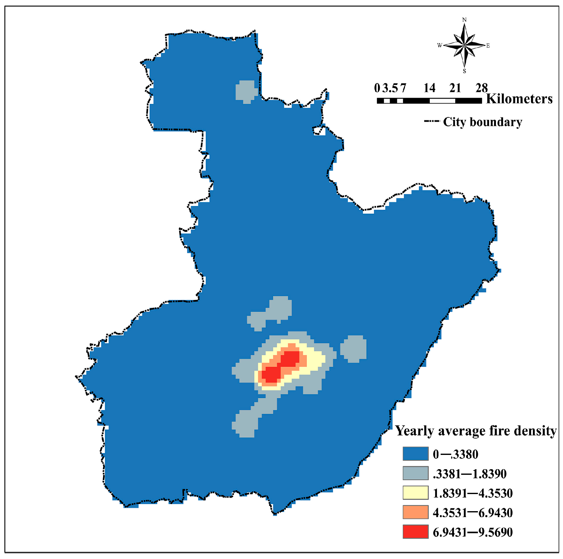
Data on the number of fires and related fire records for the period of 2002 and 2005 were obtained from the Fire Bureau in Anhui Province, China. The dataset is contained with the time of fire occurrence, location, fire damage, and related fighting time. A total of 4611 historical ignition records were found and all of them are infrastructure fires. This can be further proven, as shown in Figure 1, when most of the land use in suburban areas is cropland but not forest. The spatial distribution of fire ignition points is shown in Figure 2a. Using these data, the dependent variable was derived from the spatial estimation of kernel density, which was called yearly average fire density and indicates the ignition frequency in one grid cell (number of fires per year per km2).
In order to obtain the fire density, we adopted the kernel density method, which turns discrete points in a study area into a continuous density surface in order to prevent uncertainty and mistakes in ignition records [10]. A grid spatial resolution of 1 km2, which considers the spatial scale and a fixed bandwidth of 5 km, are used as a rule of thumb after comparing several different bandwidth values (from 1 km to 10 km) [22]. The choice of bandwidth was further evidenced by the default calculation result of kernel density by ArcGis 10.2 (ESRI, Redlands, CA, USA), which was nearly 4.7 km. Water bodies and other similar land cover types where fire cannot occur were excluded from the analysis afterwards. The resulting base grids have 6985 cells in total, covering the entire study area without water bodies; next, the centers of the pixels were used as the sample points (Figure 2b). During the initial analysis, fire was found to occur at only 752 locations at least one time after the initial statistical analysis.
2.3. Explanatory Variables: Selection and Pre-Processing
In total, 25 explanatory variables were extracted from several databases, including a variety of socioeconomic attributes according to the results in previous studies [21,23,24,25,26,27]. These variables not only consider the influence of socioeconomic conditions on fire occurrence but also consider the influence of climate and topographic conditions. These explanatory variables are shown in Table 1. In the analyses reported in this paper, values of these explanatory variables were standardized by subtracting the mean value and divided by the standard deviations of each variable.
All the explanatory variables were resampled and mapped reasonably at a 1-km2 space resolution in view of the original resolution of each variable and the spatial extent of Hefei City [22]. The main explanatory variables related to fire occurrence are shown in Figure 3. Before further analysis, Box–Cox transformation was carried out for variables in order to satisfy the statistical assumption of linear regression. What is more, multicollinearity between explanatory variables was assessed. The variables that represent different types of land use were converted into dummy variables and LANDOTHER was treated as the control predictor. Correlation coefficients that were too high (more than 0.75) were used as the criterion to remove explanatory variables [10,12]. In addition, data standardization was done during the pre-processing for training RF models with the “center” and “scale” methods in RStudio (R Development Core Team, Boston, MA, USA) [28].
2.4. Method
Considering the characteristic of spatial data such as the dependence and heterogeneity, some indicators including Moran’s I and Geary’s C index were used in the analysis of global autocorrelation for natural complex phenomena. The global and local Moran’s I are shown in Equations (1) and (2), and the related Z score of local Moran’s I is shown in Equations (3) [15]:
where is the number of spatial units; and are the values of variable in spatial unit and ; is the average over all spatial units of the variable. is the spatial weight matrix that measures the strength of the relationship between two spatial units. The index value of global Moran’s I falls between −1.0 and 1.0. The global spatial autocorrelation tool is an inferential statistic, which means that the results of the analysis are always interpreted within the context of its null hypothesis. However, the global Moran’s I does not indicate where the clusters are located or what type of spatial autocorrelation is occurring. Therefore, the local Moran’s I was calculated and the significance test of local Moran’s I was applied with a local Z test as an indicator of local spatial association, as shown in Equation (3). In addition, the correlative value of significance level could be calculated from the local Z test at different significance levels including 0.01, 0.05, 0.1, etc. What is more, if the value of Zi is positive and the local Moran’s Ii is significant, then the result indicates that the spatial units with higher values are surrounded by neighboring units, which indicates positive local spatial autocorrelation. After detailed analysis for the existence of global and local spatial autocorrelation, SE models were used accordingly. Based on such early-stage preparation of cross-sectional data, SE models are being utilized more and more widely due to their advantages compared with traditional multiple linear regression [30]. Before making decisions about which of the SE models is best, Moran’s I was tested for the response variable and SE models would be trained first in each subsample in order to find the significant explanatory variables according to the Student’s t-test. Each significant variable should fulfill the criteria of p < 0.05 and the variables selected in the final SE model should be presented at least three times in the five initial SE training models.
Firstly, we conducted the Moran’s I test in the 6985 sample points and the spatial autocorrelation of fire density was managed before we could adopt SE models in this research. The map of local Moran’ I index was extracted and calculated with the “localmoran” function in R studio and spatial weight matrix was obtained. We can find the local regions where spatial clustering of fire occurrence is significant or not, as well as the hot points where fire happens most. In this paper, we adopted ‘‘KNN (K-nearest-neighbor)’’ as the method for building a spatially weighted matrix and 8 as the K value, which means the nearest eight neighbors around a single sample point were assigned a value of 1 in the spatially weighted matrix. Afterwards, we divided the whole sample dataset into five folds by using “createMultiFolds” function in R studio. Each sample fold was used as the testing set in turn and thus we could get five intermediate models by referring to the ideas of cross-validation. This means that 80 percent of samples were used as the training set and the other 20 percent of samples were the testing set; both SE and RF models were trained five times, and thus five intermediate models for these two regression methods were obtained. Each training set has 5588 sample points and each testing set has 1397 sample points.
In addition, SE models have three basic patterns, SEM, SLM, and SAC, as shown in Equations (4)–(6). Moreover, SDM is developed with the extension of SAC, which considers spatial lagging between explanatory variables, as shown in Equation (7). All of the SE models are parametric models, whose coefficients can be obtained accordingly. After pre-processing for the explanatory models, SDM, SEM, SLM, and SAC were implemented in this study using the packages of “sp” and “spdep”; “train”, “lagsarlm”, “errorsarlm”, ”knearneigh” and “nb2listw” functions were employed in RStudio (R Development Core Team, Boston, MA, USA) [28]. R is an open-source software widely used in spatial analysis and prediction due to its advanced integration with GIS and other data formats [31]. The packages and functions mentioned above were all applied because of their excellent performance on spatial econometrics. The formulations of SE models are shown below [30]:
SEM:
where means the vector of response variable, means the matrix of independent predictors, reflects the coefficient matrix of , means the vector of random error term, means the coefficients of spatial random error terms for the vector of cross-sectional response variable, means the spatial lag of , means the vector of random error term under normal distribution.
SLM:
where means the vector of response variable, means the matrix of independent predictors, reflects the coefficient matrix of , means the vector of random error term, means the coefficients of spatial regression terms, means the spatial weight matrix, means the spatial-lag response variable.
SAC:
where means the vector of response variable, means the matrix of independent predictors, reflects the coefficient matrix of , X means the vector of random disturbance term, means the coefficients of spatial regression terms, means the spatial weight matrix, means the spatial-lag response variable, means the coefficients of spatial random error terms for the vector of cross-sectional response variable, means the spatial lag of , and means the vector of random error term under normal distribution.
SDM:
where means the vector of response variable, means the matrix of independent predictors, reflects the coefficient matrix of , means the vector of random disturbance term, means the coefficients of spatial regression terms, means the spatial weight matrix, means the spatial-lag response variable, means the coefficients of spatial random error terms for the vector of cross-sectional response variable, means the spatial lag of , and means the vector of random error term under normal distribution.
On the other hand, as other studies have depicted before, RF has become one of the most important machine learning methods based on ensemble learning [2,8,32,33,34]. It is developed as the extension of decision trees [35]. This algorithm applies random binary trees that use a subset of the observations through bootstrapping techniques. From the original dataset, a random choice of the training data is sampled and used to build the model accordingly, and the data not included are referred to as an “out-of-bag” (OOB) dataset [2,10]. This adds the element of randomness to bagging trees so as to make it less sensitive to variability in calibration such as outliers and data changes [6]. It is also an extension of bagging trees because it adds random sampling to predictors in each subset, not only in sample sets. However, this method behaves as a “black box” since the individual trees cannot be examined separately and it calculates neither regression coefficients nor confidence intervals [10]. Nevertheless, it allows for the computation of variable importance measures, which can be compared to other regression techniques. The studies before usually adopted %IncNodePurity and %IncMSE as the statistics for evaluating the importance of variables in the RF model [10,36,37].
In addition, we used the technique called “recursive feature elimination (RFE)” in RStudio software in order to get the optimal number of predictors that should be included in the model. The detailed description of RFE algorithm is offered in the help section of the “caret” package in RStudio. What is more, by making use of such nonparametric techniques (formally called CART (classification and regression trees)), RF improves a lot on the level of accuracy and prediction and this advantage could offer technical support in the process of modeling fire occurrence. In this paper, we used “train”, ”rfFuncs”, “randomForest” and “rfeControl” function in “caret” package to select variables and get the initial five RF intermediate models. All of these operations were carried out on the RStudio software platform (R Development Core Team, Boston, MA, USA).
As specified before, different SE and RF models were trained and compared in order to get the final SE and RF models. They were validated afterwards in the testing set to examine the predictive ability for fire occurrence. Statistical results such as log likelihood, Akaike information criterion (AIC), coefficient of determination (R squared), root mean square error (RMSE), and correlation coefficient were obtained for the purpose of selecting the best model. Moreover, as a comparison in this paper, the RF model was also calibrated and optimized according to the criterion of %IncNodePurity, for which could assume that predictors with a greater value have higher importance [38,39]. %IncNodePurity relates to the loss function with which the best splits are chosen. The loss function is RMSE for regression and Gini impurity for classification. More useful variables achieve higher increases in node purities, through which we can find a split that has a high outer node “variance” and a small intra node “variance.” The final variables selected in the RF model can be chosen according to the average value of %IncNodePurity within five intermediate models. Finally, the SE and RF models were fitted in the whole dataset and the residuals of the two models were extracted from the prediction results.
As presented in the research before, if no autocorrelation remained in the residuals of the regression models, then the spatial pattern observed in the dependent variable could be explained by the spatial pattern observed in the predictors [10]. Based on such prior knowledge, semivariograms of the residuals produced by different regression models were derived and these residuals were further visualized with different colors in order to examine the heterogeneity and unsteady performance. What is more, the correlations between the common predictors in both models and the residuals of each method were discussed in order to explore the factors that affected the generation of residuals.
Lastly, the maps of likelihood of fire occurrence predicted using RF and SE models were obtained by normalization of the fire density. Maps of the likelihood of fire occurrence were plotted as a comparison for each model, making it easier for people to understand the probability of ignition from the perspective of fire science.
3. Results
3.1. Dependent Variable
Figure 4 shows the yearly average fire density for the period 2002–2005, obtained using the kernel density method. A more detailed analysis revealed only 752 ignition points where fire occurred at least once, while the average value of fire density was nearly 0.15.
3.2. Explanatory Variables
Box-Cox transformation was applied in variables and the natural logarithm transformation was finally adopted for the response variable. After the multicollinearity diagnostics, four explanatory variables were excluded, including TEMMAX, TEMAVE, LANDOTHER, and ENTERTAINMENT, because of their high inter-correlations. Correlations among the explanatory variables were calculated through “corrgram” package in RStudio. The variance inflation factor (VIF) values of these explanatory variables except for the land use variables were obtained. There was no VIF value bigger than 10, as the largest one was 5.01, and this result indicated that there was no multicollinearity between predictors. The variables included in the initial training process were DEM, SLOPE, ASPECT, POSTION, TRI, SHADE, NDVI, TEMMIN, POPULATION, LINE, RESIDENT, HOTEL, EDU, MARKET, ENTERPRISE, DW, DF, DR, LAND11, LAND14, LAND2030, and LAND190.
3.3. Results of Spatial Econometric Models
The value of Moran’s I for the response variable was calculated and the results indicate that there is significant spatial autocorrelation. The value of global Moran’s I is 0.7108 and the value of P is less than 0.0000001, which means there are significant clustering patterns and the spatial distribution of feature values is not the result of random processes. Furthermore, the value of local Moran’s I, as well as the related P and Z value, is shown in Figure 5. The value of Moran’s I offers evidence for using the SE model accurately because of the existence of spatial autocorrelation.
As shown in Figure 5, most of the sample points have a value of P larger than 0.05, especially outside the urban regions, whereas the urban regions are mostly at the level of p < 0.05, which means that fire usually clusters as “high–high” in the urban regions, demonstrated by the yellow and red sample points, called “hot points” as shown in Figure 5. The green points in Figure 5b indicate that they are not significant. From the results above, the local characteristics of fire occurrence were studied, paving the way for the following modeling process.
In order to obtain the result of spatial econometric models, five intermediate SE models, SAC, SEM, SDM, and SLM, were initially built in each of the five training sets and the statistics of variables were calculated accordingly. After the preprocessing of data and statistical tests, SE models were obtained (summary shown in Table 2). The result shows that SAC is the best SE model considering its lowest value of AIC and highest log likelihood, which means SAC could explain most of the variance in the model and the fitness of SAC is higher than other SE models. We could also infer from the result that the spatial autocorrelation not only exists in response variable but also in the random error term. The values of related parameters in SAC including and are −0.78 and 0.97, respectively.
A summary of the five SAC intermediate models is shown below and a summary of predictors is also obtained (see Table 3). The results indicate that LINE, TEMMIN, DEM, and DF (with confidence level of 0.05) are selected in the final SAC model and the spatial distribution of LINE has a positive effect on fire occurrence for the SAC model while the other three selected predictors are the opposite. Meanwhile, according to the absolute value of predictors in Table 3, LINE influences the SAC model most, followed by TEMMIN, DEM, and DF.
The final SAC model was fitted using the above selected predictors and the summary of SAC is shown in Table 4. We could infer from the results that LINE plays the most important role in modeling fire occurrence for SAC; TEMMIN ranks the second, followed by DEM and DF. Although DEM and DF are significant in the model, their coefficients are so small that physical factors and the nearest distance from sample points to fire stations do not have a significant effect on infrastructure fire occurrence. This seems reasonable because DF does not affect fire occurrence directly with spatial econometric models but can only reflect to some extent whether the sample point is in an urban area or not.
As for the validations among each training set and testing set, the correlations were calculated and shown in Table 5. The result shows that each SAC intermediate model has a good predictive ability among each training set but its robustness is not good according to the low value of correlation in each testing set. This may point to a dependence on the special structure of spatial weight matrix and the coefficients of predictors may not be the same at each location, which may lead to an error in the prediction for a new dataset.
3.4. Results of Random Forest Model
Just as for the SAC model, five intermediate RF models were calculated by using the same training sets and the importance of each predictor was obtained in order to select the final RF model. The predictors are ranked in descending order according to the value of average %IncNodePurity among five intermediate RF models, as shown in Table 6. The rank order for different predictors indicates that it is very different from what is shown in the SAC model. DF ranks first and POPULATION is second, and followed by LINE, ENTERPRISE, TEMMIN, and DEM. LINE, DF, DEM, and TEMMIN are common variables in both models, from which we could infer that the four predictors play an important role in modeling fire occurrence and are not sensitive to the different pattern of models.
The importance of each predictor in five intermediate RF models was extracted and ranked in descending order, as shown in Figure 6. As shown in Figure 6, the order of different predictors is not the same and the importance of a predictor may vary between training sets. Moreover, Figure 6 shows that among all the 22 variables, the rank order of the front six predictors, which have a large value of %InNodePurity, are not the same. What is more, if we delete the other 16 variables, the whole degree of fitting in RF is not changed much, which only decreases by less than 2%. Finally, we adopted DF, POPULATION, ENTERPRISE, LINE, TEMMIN, and DEM as the predictors in the final RF model. The selection criterion for the value of %InNodePurity is about 40,000 according to the calculation result of RFE, from which the optimal number of variables is obtained as 6.
As for the validations among each training set and testing set, the correlations were calculated and shown in Table 7. The result shows that the RF model has a good predictive ability both on each training set and testing set. This may point to the robustness of the non-parametric model and its excellent prediction for new data.
3.5. Results of the Correlations for Both Final Models
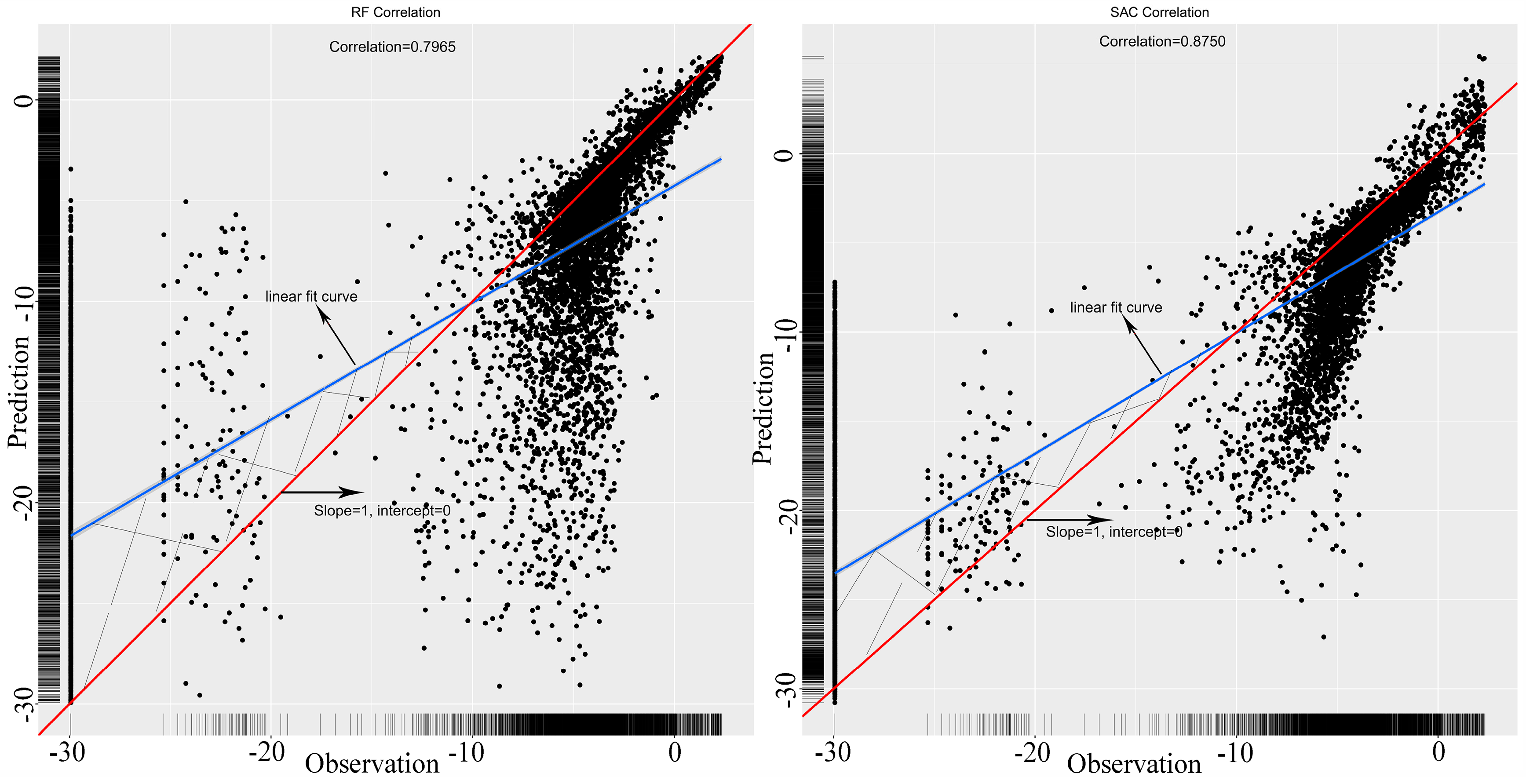
The final SAC and RF model were fitted for the whole sample data using selected predictors and the correlations between the observed fire density and predicted value, as shown in Figure 7. The red line means the correlation between the observed and the predicted is 1 and the blue is the linear fit curve. The figure shows that SAC has a higher value of correlation at 0.875 than RF, whose correlation value is 0.797, evidenced by the smaller included angle for SAC. What is more, the trend line of correlation has a decreasing tendency for both RF and SAC, which means these points below the red line are underestimated. What is interesting is that there exist some random dispersive points that have a very small value of fire density in the left area of the plots. This shows that the prediction result is mainly dominated by a high density of fires within the urban areas, while it is difficult to predict areas far from the city. The rural and suburban areas have a small probability of fire occurrence. This phenomenon indicates that RF and SAC cannot predict well on all points neither, especially for points seldom at risk of fire, but models are efficient for the points under high fire risk.
3.6. Spatial Autocorrelation for Residuals among Different Models
After the above analysis, a spatial autocorrelation test for residuals was performed and visualized for the whole study area. We divided the value of residuals into five quantiles as the minimum, 25%, 50%, 75%, and the maximum, and then each quantile was colored with light green, green, yellow, red, and black. In Figure 8, the light color points represent the sample points with underestimations, while the dark ones represent overestimations, as shown in Figure 8. Moreover, it is easy to find that regions covered with underestimated points (light color) for SAC are exactly where covered with overestimated points (dark color) for RF.
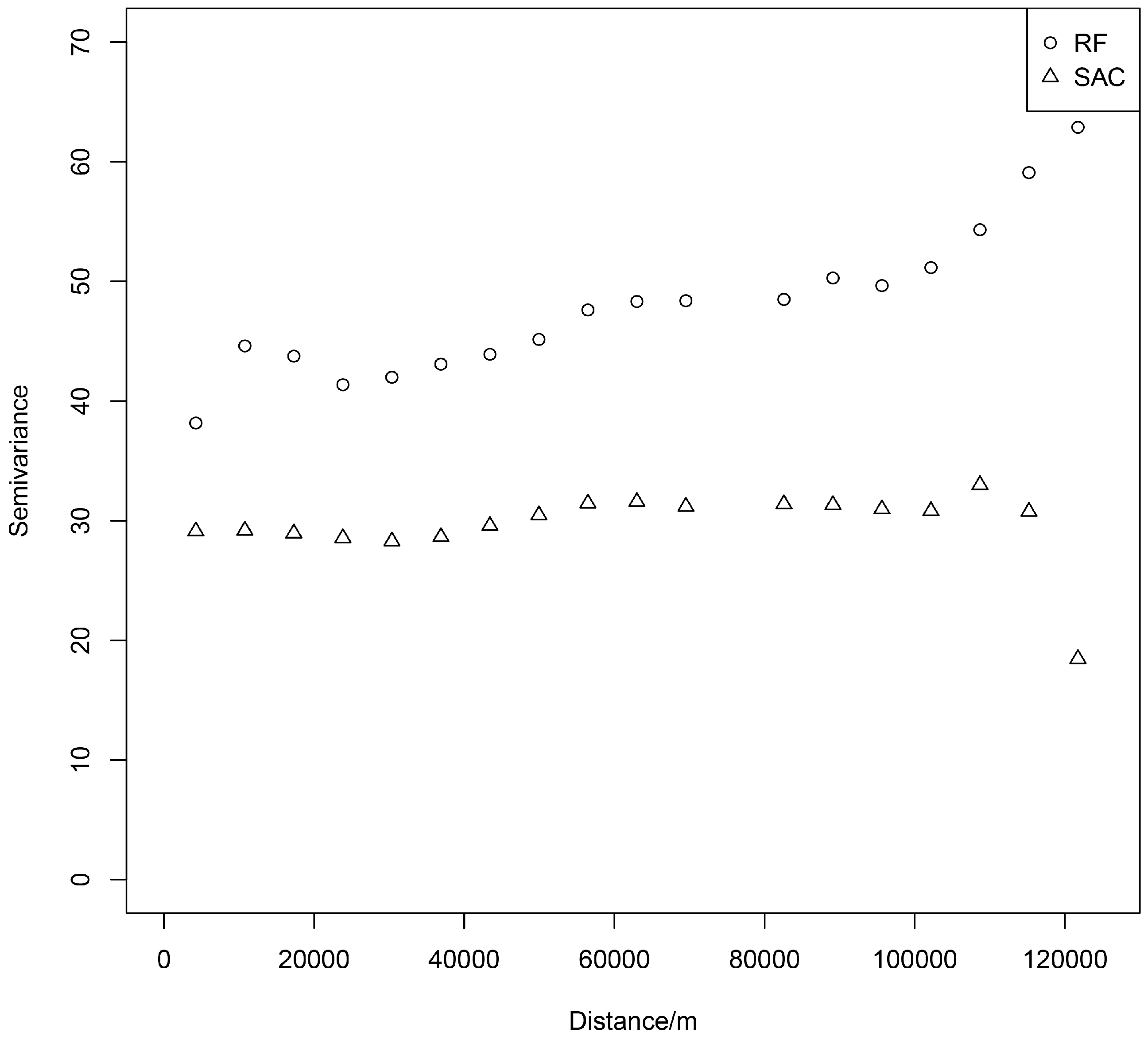
The semivariograms are presented in Figure 9. They indicate that SAC performs better than RF when considering the ability to explain the spatial structure. In detail, the semivariogram plots of SAC show relatively stable trends and a lower value when compared with RF. Moreover, after the break point of nearly 20 km, the value of the semivariograms decreased for both models. This means the spatial autocorrelation of residuals increases to a distance of 20 km. The semivariogram plot of RF shows an increasing trend in general, while SAC is steady and the value of semi-variance decreases after about 110 km. The result shows that the SAC model is better at modeling the occurrence of infrastructure fires and also explaining the spatial structure of fires at the city scale.
3.7. Correlations between Common Variables and Residuals in RF and SAC
As shown above, SAC is better than RF when concentrating on its good predictive performance. A deeper analysis of the correlations between the residuals and the common variables in both SAC and RF models will increase our understanding of the reasons why prediction errors are generated. Therefore, as shown in Figure 10, we could find some useful potential regularity by taking SAC as an example. As shown in Figure 10a, most of the residuals are skewed to the left, and the corresponding value of LINE is between 0 and 0.30. This shows that regions with low road density may be not as reliable as regions with high road density for predicting the probability of fire occurrence. The regions where people have limited access may be hard for models to make efficient predictions. On the other hand, the residuals are skewed to the right, as shown in Figure 10b, which indicates that the residuals are generated when the value of TEMMIN is between 0.60 and 0.90. The regions with high temperature may contribute to prediction residuals and could help explain the heat island effect in urban areas. We can also infer from Figure 10c that most residuals are skewed to the left because regions with low elevation may be easier for human beings to settle in and the clustering of humans and their activities will create the conditions necessary for fire to occur. However, the flatlands may be not beneficial for predicting fire occurrence at the city scale, which contribute significantly to the generation of residuals. The last predictor is DF, which means the nearest distance to fire stations and can indirectly reflect the efficiency of the fire prevention and emergency response, as shown in Figure 10d. Figure 10d shows that the residuals are evenly dispersed across almost the whole range of DF.
3.8. Maps of the Likelihood of Fire Occurrence
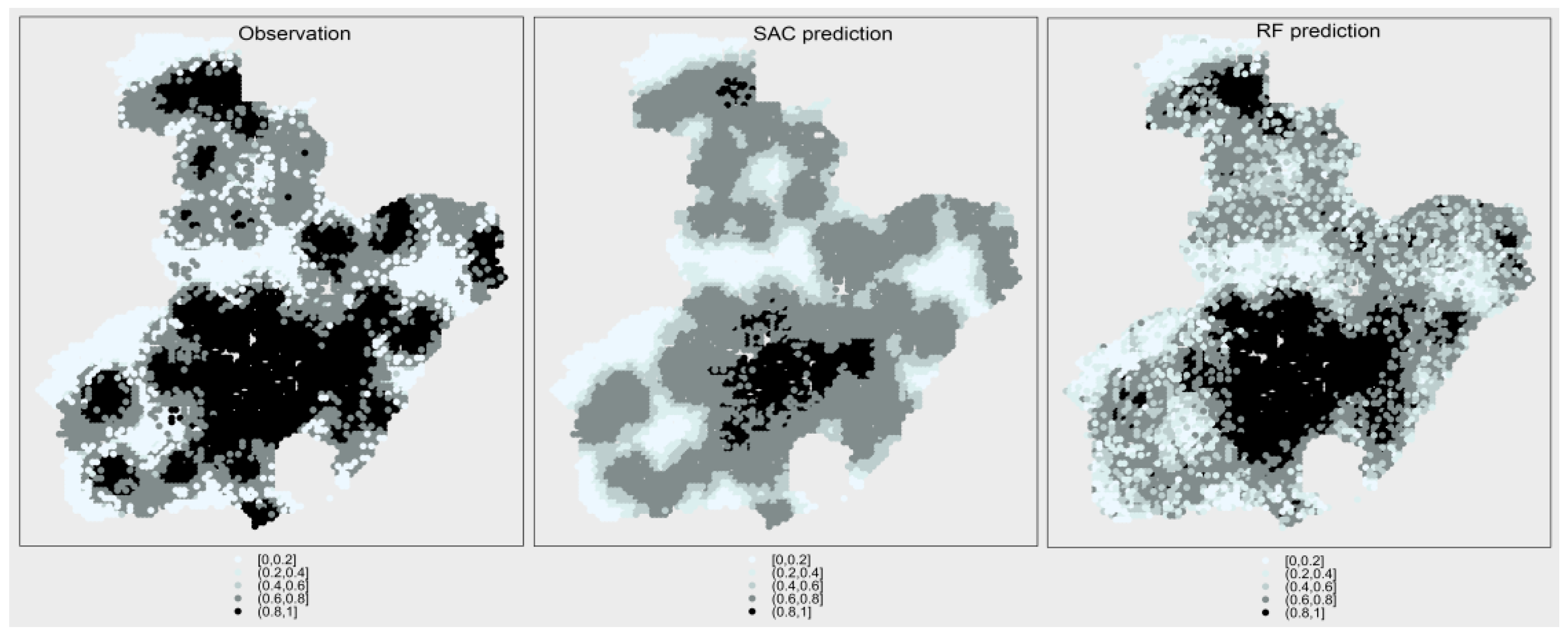
The likelihood of fire occurrence was normalized by transforming fire density into a variable ranging from 0 to 1. Figure 11 shows, in the left panel, the actual fire density, the value predicted by SAC (middle panel), and the value predicted by RF (right panel). We can infer from the figure that SAC could describe the approximate shape of fire occurrence, while RF could not. Moreover, most of the sample points were underestimated for SAC, while RF could make good predictions of the points with high risk value but the spatial boundaries of the predicted fire density were not as clear as with SAC. This means that both SAC and RF have their strengths and shortcomings and the predictive performance of each model changes in different city areas. A deeper analysis shows that the values of correlation coefficient between observed and predicted are 0.875 and 0.797 for SAC and RF, respectively. This indicates that the spatial distribution characteristics of fire occurrence are better explained by SAC than by RF on the whole.
3.9. Comparison with Other Fire Models
Different spatiotemporal scales, approaches to spatial sampling, and study regions can affect which model to choose and the performance of models [40]. Wildfires have close correlation with physical factors, climate factors, and the activities of human beings. However, as to urban infrastructure fires, the important predictors are much different and, therefore, the measures for preventing infrastructure fires from happening will be very different too. We should not deny that the occurrence of fire often shows spatial and temporal clustering and lagging [41,42,43]. Moreover, many natural phenomena such as chemical toxicants and PM 2.5 are spatially auto-correlative and the SE model is a useful tool for explaining the structure of natural hazards [44,45,46,47,48]. Therefore, when analyzing natural phenomena and trying to find key predictors, we should be cautious and adopt a specific model only after sufficient investigation.
3.10. Limitations
This study has several limitations that may influence the results. First, because of the constrained access to a wider range of relevant variables, more explanatory variables need to be considered and explored in future studies. In particular, we should pay more attention to other socioeconomic predictors such as the spatial distribution of POIs, since these factors may have a significant influence on fire occurrence at the city scale. Second, as fire risk is always changing and its spatial distribution varies with the development of a city, fire risk in urban areas is considerably different from wildfires in forest regions. Therefore, the predictors should take into account these dynamic characteristics. Third, fire occurrence is an integrated process where time and space are integral dimensions. This means that the varying-coefficient models such as geographic temporally weighted regression or geographic weighted regression should be contrasted with SAC or global models. Other limitations such as the parameter tuning process, running time, and feature selection should also be recognized in order to construct more suitable models.
4. Conclusions
This paper compares SE and RF models for studying fire occurrence at the city scale. As regards the applicability of models, we found that RF performed better than SAC in predicting a new dataset with more robustness. Cross-validation was employed and the relatively important predictors were included for both models. On the other hand, SAC showed an efficient ability for explaining the spatial structure of fire occurrence because of its functional equation, which could effectively eliminate the autocorrelation in the residual terms.
Global and local spatial autocorrelation were tested using Moran’s I index; the results showed that there was significant global spatial autocorrelation for the average density of infrastructure fires. In addition, significant local autocorrelation mostly clusters in urban areas. Therefore, we could use SE models to perform further analysis of the distribution patterns and spatial structure of fire occurrence at the city scale. Afterwards, the statistics of each predictor among SE models was examined by using the ideas of five-fold cross-validation in terms of the accuracy of prediction in each training set. Five intermediate models for SEM, SLM, SDM, and SAC were obtained and SAC was selected because of its lowest AIC value and highest log likelihood. Afterwards, LINE, TEMMIN, DEM, and DF were selected in the final SAC model. The predictive performance in each training set and testing set for SAC was obtained and the results showed that SAC could predict well in the five training sets but rather poorly in the new datasets. This was caused by the special principle of spatial weight matrix based on the spatial structure of sample points as well as the spatial heterogeneity.
As regards RF, we used the same procedure for SAC and five intermediate models were examined for selecting the predictors in the final RF model. The predictive performance in each training set and testing set was obtained and the results showed that RF performed well in both training sets and testing sets. In comparison with SAC, RF is not sensitive to the spatial structure of sample points and thus could make robust predictions for new datasets. However, RF lacks the ability to explain the spatial structure of fire occurrence and thus the correlation values in five training sets are smaller than with SAC. We adopted DF, POPULATION, ENTERPRISE, LINE, TEMMIN, and DEM as the predictors selected in the final RF model.
We fitted the whole dataset by using the final RF and SAC model, and the correlation value between the observed and the predicted is 0.7965 and 0.8750, respectively. What is interesting is that there are some random dispersive points in plots whose value of fire density is small. This phenomenon indicates that RF and SAC cannot predict well on all sample points, especially for points seldom at risk of fire, but both models are efficient for points under high fire risk.
With respect to the spatial autocorrelation of residuals, SAC is much better than RF. A comparison of model performance between RF and SAC showed that SAC is better at fitting fire risk and explaining the spatial structure in terms of the flat trend and a lower level of semivariogram function.
The common variables selected in both models were analyzed for the correlation with the residuals predicted in SAC. The results showed that areas with low road density may be not as reliable as those with high road density for predicting fire occurrence. In areas where people have limited transportation access it may be hard for the models to make efficient predictions. High temperature may be one contributor to the residuals generated by prediction. We could also infer that most residuals are associated with regions of low elevation, where it may be easier for human beings to settle and the clustering of humans and their activities will create the necessary conditions for fire occurrence. However, flatlands may be not beneficial for predicting fire occurrence and are one of the contributors to residuals. The last predictor, DF, which represents the nearest distance to fire stations, may reflect the efficiency of the fire prevention and emergency response. The residuals are evenly dispersed across the whole range of DF.
Furthermore, at the city level, we should focus on the redistribution of POIs highly correlated with human abilities and make more discoveries about the estimation of the source of danger, especially for the purposes of fire prevention. RF could be an efficient tool for decision makers to make forecasts. Moreover, SAC could be applied after a sufficient exploration of predictors for a specific city when there is spatial autocorrelation or a hysteresis effect.
In future, we should adopt dynamic approaches for predicting and estimating the quantitative fire risk within each grid cell. However, the ability to explain the spatial structure using spatial econometric models should not be ignored. In addition, other predictors associated with fire risk should be included in the study in order to find better ways to analyze fire risk from a spatiotemporal perspective. Lastly, predictors that have close correlation with humans should be carefully examined.
Acknowledgments
The authors are grateful for financial support from the China Scholarship Council. This work was also sponsored by the National Key Research and Development Plan (Grant No. 2016YFC0800601, 2016YFC0800100) and the Fundamental Research Funds for the Central Universities of China (Grant No. WK2320000033, WK2320000036). The authors are also grateful to the Fire Bureau of Anhui Province, China, from which researchers can obtain historical fire records. This work was also supported in part by the National Natural Science Foundation of China (grant number 41529101) and by grant 1-ZE24 (Project of Strategic Importance) from Hong Kong Polytechnic University.
Author Contributions
Chao Song did the majority of the work and wrote this paper; Mei-Po Kwan offered valuable suggestions on geography and English polishing; Weiguo Song offered valuable suggestions for this paper; Jiping Zhu is the corresponding author offering financial assistance and valuable suggestions on fire science and data sources.
Conflicts of Interest
The authors declare no conflict of interest. The founding sponsors had no role in the design of the study; in the collection, analyses, or interpretation of data; in the writing of the manuscript, and in the decision to publish the results.
References
- News Sina, China. In 2015, 1742 Persons Were Recorded as Dead Because of Fire. Available online: http://news.sina.com.cn/c/2016-01-18/doc-ifxnqriy3078516.shtml (accessed on 12 May 2017).
- Pourtaghi, Z.S.; Pourghasemi, H.R.; Aretano, R.; Semeraro, T. Investigation of general indicators influencing on forest fire and its susceptibility modeling using different data mining techniques. Ecol. Indic. 2016, 64, 72–84. [Google Scholar] [CrossRef]
- Modugno, S.; Balzter, H.; Cole, B.; Borrelli, P. Mapping regional patterns of large forest fires in wildland–urban interface areas in Europe. J. Environ. Manag. 2016, 172, 112–126. [Google Scholar] [CrossRef] [PubMed]
- Chas-Amil, M.L.; Prestemon, J.P.; McClean, C.J.; Touza, J. Human-ignited wildfire patterns and responses to policy shifts. Appl. Geogr. 2015, 56, 164–176. [Google Scholar] [CrossRef]
- Zhang, H.; Qi, P.; Guo, G. Improvement of fire danger modelling with geographically weighted logistic model. Int. J. Wildland Fire 2014, 23, 1130–1146. [Google Scholar] [CrossRef]
- Rodrigues, M.; de la Riva, J. An insight into machine-learning algorithms to model human-caused wildfire occurrence. Environ. Model. Softw. 2014, 57, 192–201. [Google Scholar] [CrossRef]
- Naghibi, S.A.; Pourghasemi, H.R.; Dixon, B. Gis-based groundwater potential mapping using boosted regression tree, classification and regression tree, and random forest machine learning models in Iran. Environ. Monit. Assess. 2016, 188, 1–27. [Google Scholar] [CrossRef] [PubMed]
- Reid, C.E.; Jerrett, M.; Petersen, M.L.; Pfister, G.G.; Morefield, P.E.; Tager, I.B.; Raffuse, S.M.; Balmes, J.R. Spatiotemporal prediction of fine particulate matter during the 2008 Northern California wildfires using machine learning. Environ. Sci. Technol. 2015, 49, 3887–3896. [Google Scholar] [CrossRef] [PubMed]
- Rodrigues, M.; de la Riva, J.; Fotheringham, S. Modeling the spatial variation of the explanatory factors of human-caused wildfires in Spain using geographically weighted logistic regression. Appl. Geogr. 2014, 48, 52–63. [Google Scholar] [CrossRef]
- Oliveira, S.; Oehler, F.; San-Miguel-Ayanz, J.; Camia, A.; Pereira, J.M.C. Modeling spatial patterns of fire occurrence in Mediterranean Europe using multiple regression and random forest. For. Ecol. Manag. 2012, 275, 117–129. [Google Scholar] [CrossRef]
- Martínez-Fernández, J.; Chuvieco, E.; Koutsias, N. Modelling long-term fire occurrence factors in Spain by accounting for local variations with geographically weighted regression. Nat. Hazards Earth Syst. Sci. 2013, 13, 311–327. [Google Scholar] [CrossRef]
- Song, C.; Kwan, M.P.; Zhu, J. Modeling fire occurrence at the city scale: A comparison between geographically weighted regression and global linear regression. Int. J. Environ. Res. Public Health 2017, 14, E396. [Google Scholar] [CrossRef] [PubMed]
- Fotheringham, A.S.; Crespo, R.; Yao, J. Geographical and temporal weighted regression (GTWR). Geogr. Anal. 2015, 47, 431–452. [Google Scholar] [CrossRef]
- Špatenková, O.; Virrantaus, K. Discovering spatio-temporal relationships in the distribution of building fires. Fire Saf. J. 2013, 62, 49–63. [Google Scholar] [CrossRef]
- LeSage, J.; Pace, R.K. Introduction to Spatial Econometrics; Chapman & Hall/Crc Press: Boca Raton, FL, USA, 2009; pp. 1–42. [Google Scholar]
- Barreal, J.; Loureiro, M.L. Modelling spatial patterns and temporal trends of wildfires in Galicia (NW Spain). For. Syst. 2015, 24, e-022. [Google Scholar]
- Jung, M.; Tautenhahn, S.; Wirth, C.; Kattge, J. Estimating basal area of spruce and fir in post-fire residual stands in Central Siberia using Quickbird, feature selection, and Random Forests. Procedia Comput. Sci. 2013, 18, 2386–2395. [Google Scholar] [CrossRef]
- Martinez, J.; Vega-Garcia, C.; Chuvieco, E. Human-caused wildfire risk rating for prevention planning in Spain. J. Environ. Manag. 2009, 90, 1241–1252. [Google Scholar] [CrossRef] [PubMed]
- Serra, L.; Juan, P.; Varga, D.; Mateu, J.; Saez, M. Spatial pattern modelling of wildfires in Catalonia, Spain 2004–2008. Environ. Model. Softw. 2013, 40, 235–244. [Google Scholar] [CrossRef]
- Corcoran, J.; Higgs, G.; Higginson, A. Fire incidence in metropolitan areas: A comparative study of Brisbane (Australia) and Cardiff (United Kingdom). Appl. Geogr. 2011, 31, 65–75. [Google Scholar] [CrossRef]
- Romero-Calcerrada, R.; Barrio-Parra, F.; Millington, J.D.A.; Novillo, C.J. Spatial modelling of socioeconomic data to understand patterns of human-caused wildfire ignition risk in the SW of Madrid (central Spain). Ecol. Model. 2010, 221, 34–45. [Google Scholar] [CrossRef]
- Vilar, L.; Woolford, D.G.; Martell, D.L.; Martn, M.P. A model for predicting human-caused wildfire occurrence in the region of Madrid, Spain. Int. J. Wildland Fire 2010, 19, 325–337. [Google Scholar] [CrossRef]
- Mourão, P.R.; Martinho, V.D. The choices of the fire—Debating socioeconomic determinants of the fires observed at Portuguese municipalities. For. Policy Econ. 2014, 43, 29–40. [Google Scholar] [CrossRef]
- Jennings, C.R. Social and economic characteristics as determinants of residential fire risk in urban neighborhoods: A review of the literature. Fire Saf. J. 2013, 62, 13–19. [Google Scholar] [CrossRef]
- Sebastián-López, A.; Salvador-Civil, R.; Gonzalo-Jiménez, J.; SanMiguel-Ayanz, J. Integration of socio-economic and environmental variables for modelling long-term fire danger in Southern Europe. Eur. J. For. Res. 2008, 127, 149–163. [Google Scholar] [CrossRef]
- Butry, D.T. Economic performance of residential fire sprinkler systems. Fire Technol. 2008, 45, 117–143. [Google Scholar] [CrossRef]
- Almeida, A.F.; Moura, P.V. The relationship of forest fires to agro-forestry and socio-economic parameters in Portugal. Int. J. Wildland Fire 1992, 2, 37–40. [Google Scholar] [CrossRef]
- Team, R.C. R: A Language and Environment for Statistical Computing; R Foundation for Statistical Computing: Vienna, Austria, 2013. [Google Scholar]
- Center for International Earth Science Information Network—CIESIN—Columbia University. Gridded Population of the World, Version 4 (gpwv4): Population Density; NASA Socioeconomic Data and Applications Center (SEDAC): Palisades, NY, USA, 2015.
- Anselin, L.; Center, B. Spatial econometrics. Companion Theor. Econo. 1999. [CrossRef]
- Brenning, A. Spatial Cross-Validation and Bootstrap for the Assessment of Prediction Rules in Remote Sensing: The r Package Sperrorest; International Geoscience and Remote Sensing Symposium (IGARSS): Anchorage, AK, USA, 2012; pp. 5372–5375. [Google Scholar]
- Tramontana, G.; Ichii, K.; Camps-Valls, G.; Tomelleri, E.; Papale, D. Uncertainty analysis of gross primary production upscaling using random forests, remote sensing and eddy covariance data. Remote Sens. Environ. 2015, 168, 360–373. [Google Scholar] [CrossRef]
- Strobl, C.; Boulesteix, A.L.; Zeileis, A.; Hothorn, T. Bias in random forest variable importance measures: Illustrations, sources and a solution. BMC Bioinform. 2007, 8. [Google Scholar] [CrossRef] [PubMed]
- Breiman, L. Consistency for a simple model of random forests. In Technical Report 670; Technical Report; Department of Statistics, University of California: Berkeley, CA, USA, 2004. [Google Scholar]
- Laha, D.; Ren, Y.; Suganthan, P.N. Modeling of steelmaking process with effective machine learning techniques. Expert Syst. Appl. 2015, 42, 4687–4696. [Google Scholar] [CrossRef]
- Genuer, R.; Poggi, J.M.; Tuleau-Malot, C. Variable selection using random forests. Pattern Recognit. Lett. 2010, 31, 2225–2236. [Google Scholar] [CrossRef]
- Menze, B.H.; Kelm, B.M.; Masuch, R.; Himmelreich, U.; Bachert, P.; Petrich, W.; Hamprecht, F.A. A comparison of random forest and its Gini importance with standard chemometric methods for the feature selection and classification of spectral data. BMC Bioinform. 2009, 10, 1–16. [Google Scholar] [CrossRef] [PubMed]
- Gislason, P.O.; Benediktsson, J.A.; Sveinsson, J.R. Random forests for land cover classification. Pattern Recognit. Lett. 2006, 27, 294–300. [Google Scholar] [CrossRef]
- Diaz-Uriarte, R.; Alvarez de Andres, S. Gene selection and classification of microarray data using random forest. BMC Bioinform. 2006, 7. [Google Scholar] [CrossRef] [PubMed]
- Falk, M.G.; Denham, R.J.; Mengersen, K.L. Spatially stratified sampling using auxiliary information for geostatistical mapping. Environ. Ecol. Stat. 2009, 18, 93–108. [Google Scholar] [CrossRef]
- Wang, D.; Lu, L.; Zhu, J.; Yao, J.; Wang, Y.; Liao, G. Study on correlation between fire fighting time and fire loss in urban building based on statistical data. J. Civ. Eng. Manag. 2016, 22, 874–881. [Google Scholar] [CrossRef]
- Lu, L.; Peng, C.; Zhu, J.; Satoh, K.; Wang, D.; Wang, Y. Correlation between fire attendance time and burned area based on fire statistical data of Japan and China. Fire Technol. 2013, 50, 851–872. [Google Scholar] [CrossRef]
- Rodrigues, M.; Jiménez, A.; de la Riva, J. Analysis of recent spatial-temporal evolution of human driving factors of wildfires in Spain. Nat. Hazards 2016, 84, 2049–2070. [Google Scholar] [CrossRef]
- Zhao, X.; Huang, X.; Liu, Y. Spatial autocorrelation analysis of Chinese inter-provincial industrial chemical oxygen demand discharge. Int. J. Environ. Res. Public Health 2012, 9, 2031–2044. [Google Scholar] [CrossRef] [PubMed]
- Kissling, W.D.; Carl, G. Spatial autocorrelation and the selection of simultaneous autoregressive models. Glob. Ecol. Biogeogr. 2007. [Google Scholar] [CrossRef]
- Dormann, C.F.; McPherson, J.M.; Araújo, M.B.; Bivand, R.; Bolliger, J.; Carl, G.; Davies, R.G.; Hirzel, A.; Jetz, W.; Kissling, W.D.; et al. Methods to account for spatial autocorrelation in the analysis of species distributional data: A review. Ecography 2007, 30, 609–628. [Google Scholar] [CrossRef]
- Telford, R.J.; Birks, H.J.B. The secret assumption of transfer functions: Problems with spatial autocorrelation in evaluating model performance. Quat. Sci. Rev. 2005, 24, 2173–2179. [Google Scholar] [CrossRef]
- González-Megís, A.; Gómez, J.M.; Sánchez-Piñero, F. Consequences of spatial autocorrelation for the analysis of metapopulation dynamics. Ecology 2005, 86, 3264–3271. [Google Scholar] [CrossRef]
Figure 1.
Location of study area and land use distribution.

Figure 2.
Ignition points and sample points from 2002 to 2005. (a) Ignition points from 2002 to 2005; (b) Sample points from 2002 to 2005.
Figure 2.
Ignition points and sample points from 2002 to 2005. (a) Ignition points from 2002 to 2005; (b) Sample points from 2002 to 2005.
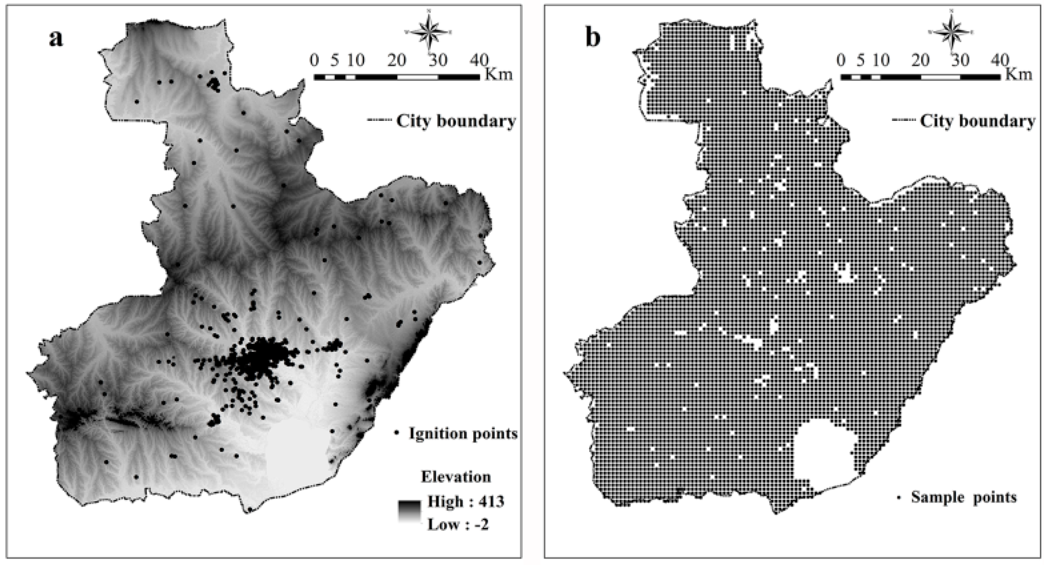
Figure 3.
Relevant main predictors including (a) nearest distance to water bodies (m); (b) fire stations and yearly average population between 2002 and 2005(people/km2); (c) density of roads (km/km2); (d) places of interests including entertainments, enterprises, education places, hotels, markets, and residential accommodations, with the background of average NDVI in 2002.
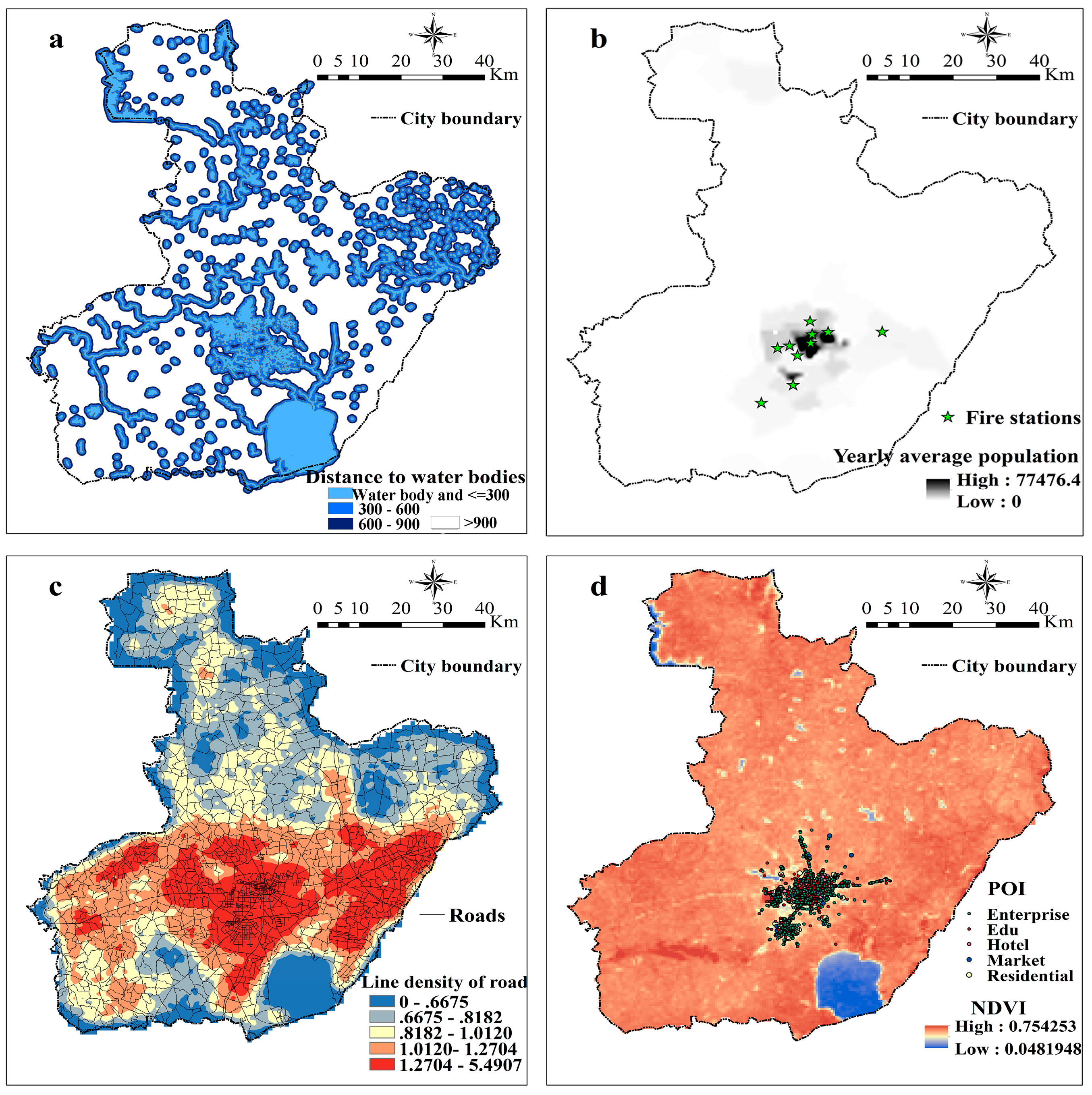
Figure 4.
Fire density calculated by using kernel density (bandwidth = 5 km).

Figure 5.
Local Moran’s I value and the related P and Z value.
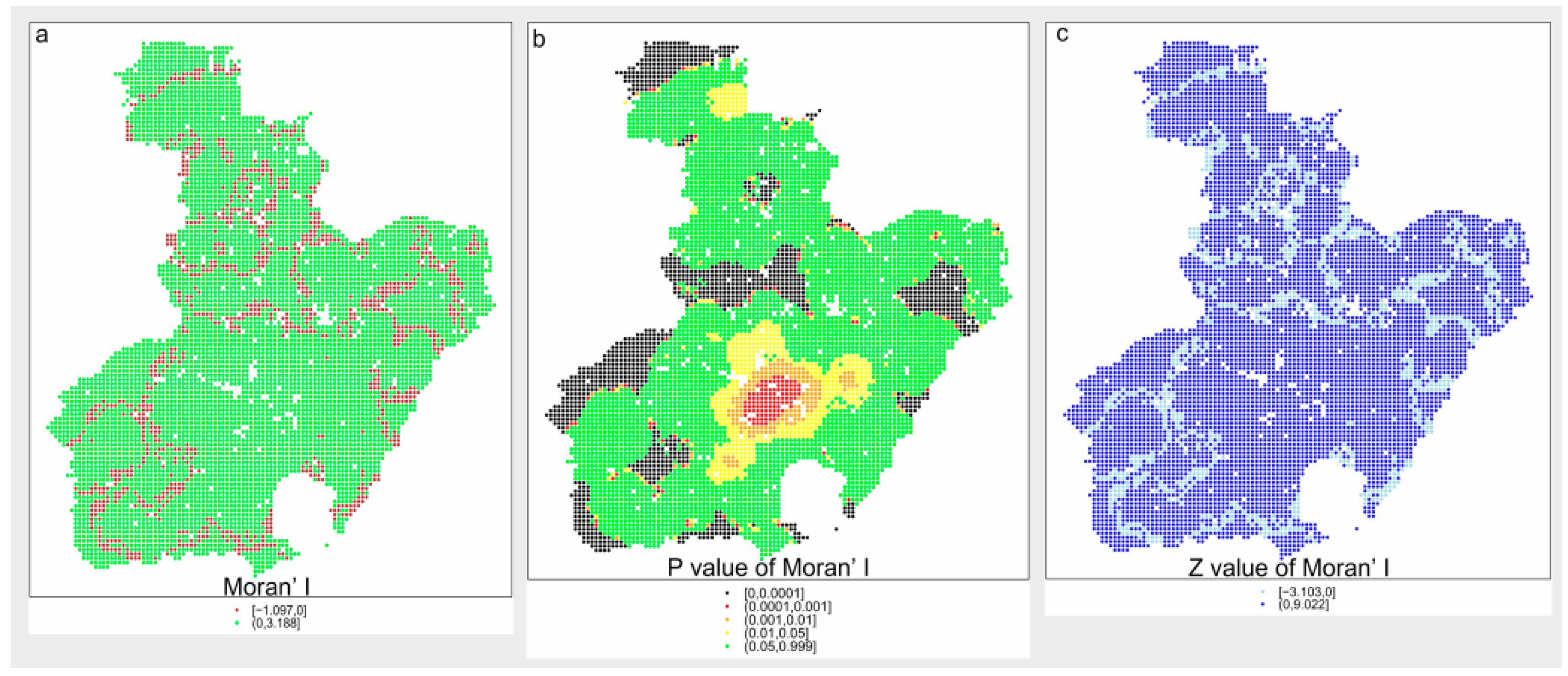
Figure 6.
The rank order for the importance measure of different predictors among five intermediate RF models.
Figure 6.
The rank order for the importance measure of different predictors among five intermediate RF models.
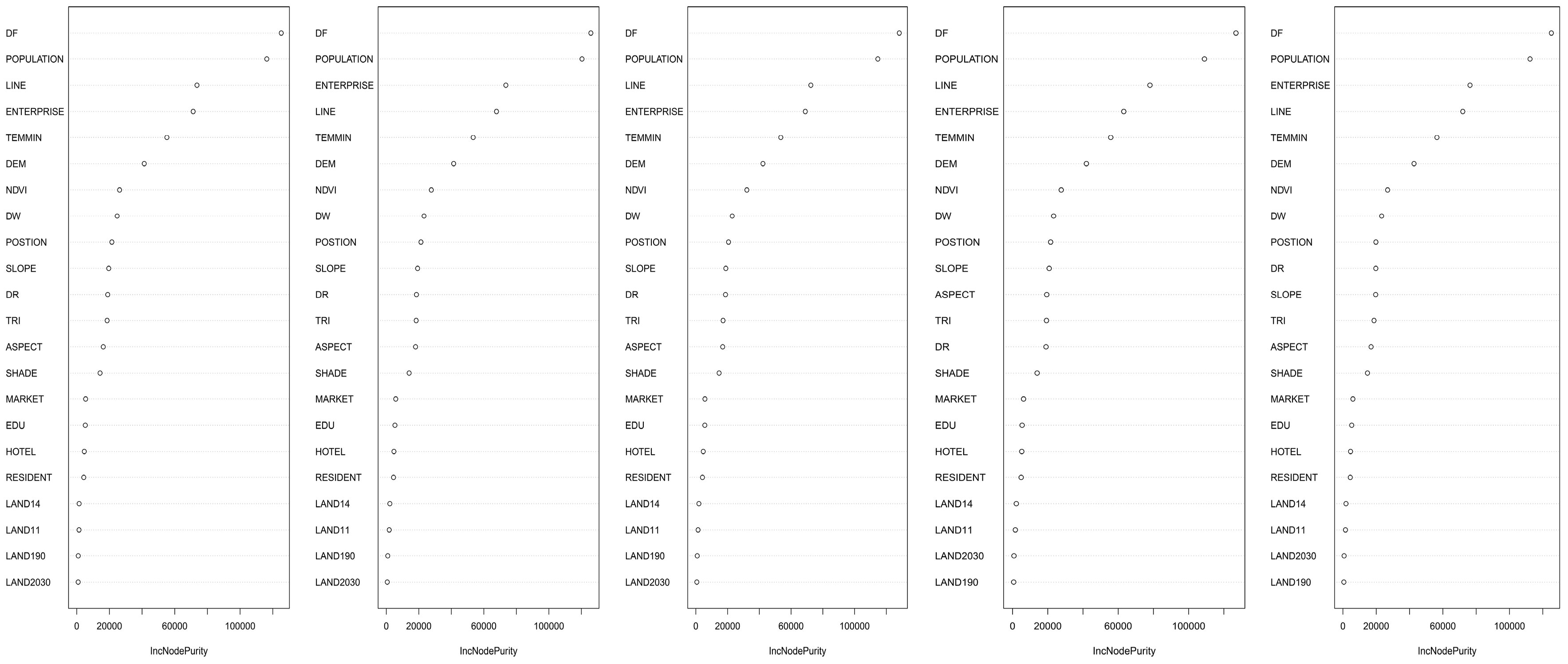
Figure 7.
The correlation plot for the final SAC and RF model in the whole dataset.

Figure 8.
Visualization of the distribution of residuals for different models.
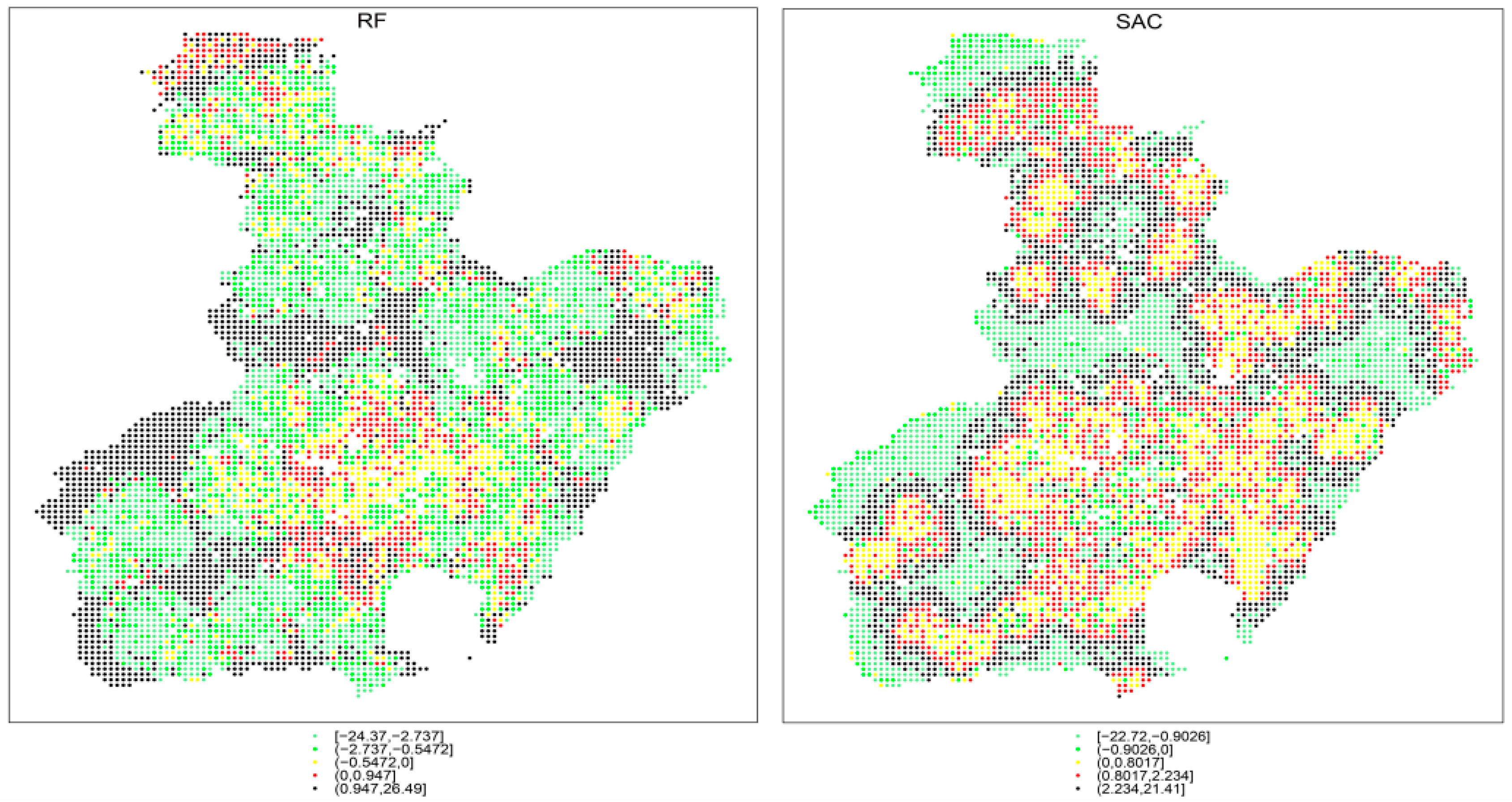
Figure 9.
Semivariogram for residuals based on the function of distance (m).

Figure 10.
Correlation plots between residuals and the predictors. The red line is the contrast line with slope = 1, intercept = 0. (a) Correlation between residuals and LINE; (b) Correlation between residuals and TEMMIN; (c) Correlation between residuals and DEM; (d): Correlation between residuals and DF.
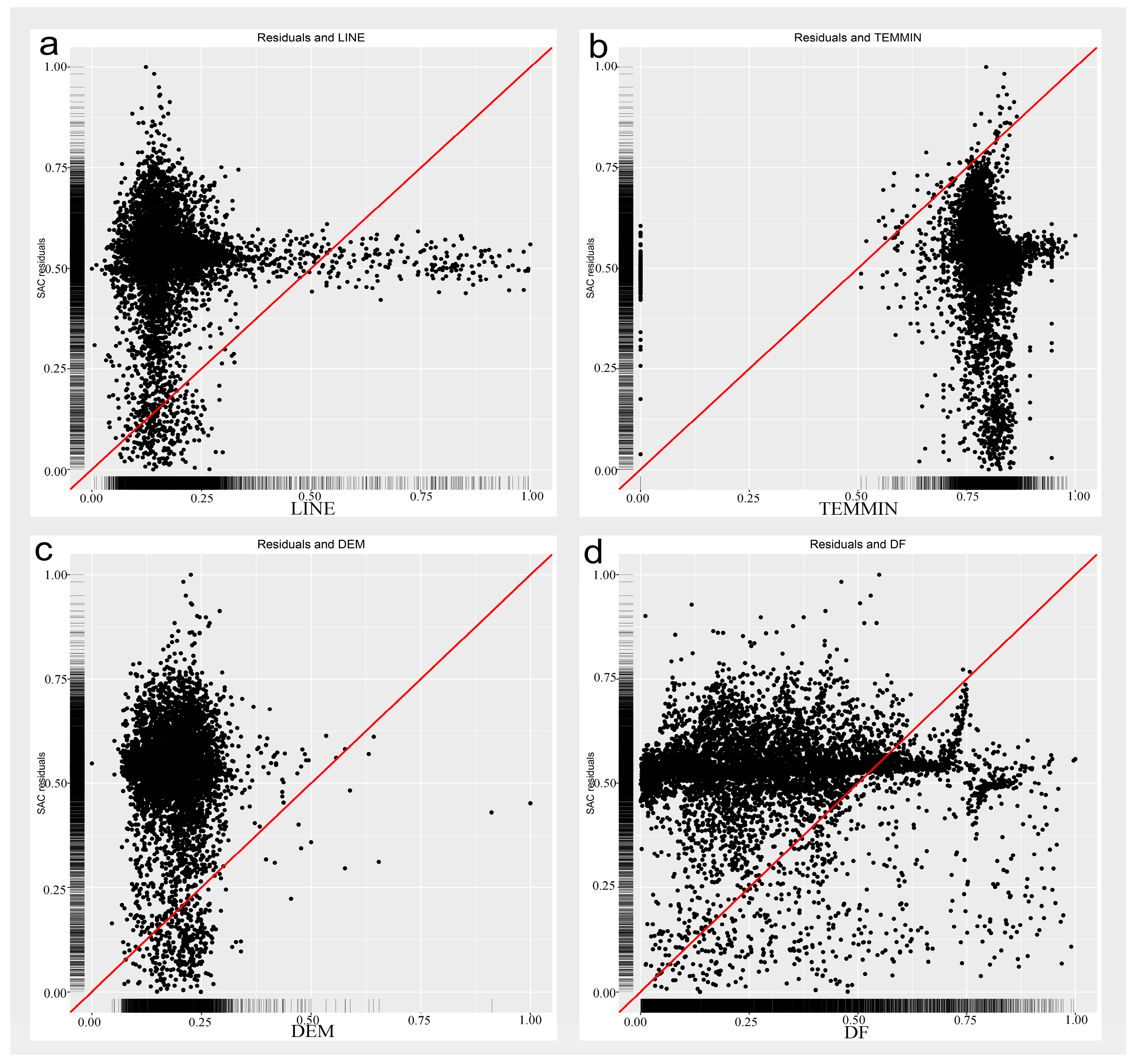
Figure 11.
Maps of the likelihood of fire occurrence. Fire density was normalized and divided into five intervals. The darker the color, the greater the probability of fire occurrence.
Figure 11.
Maps of the likelihood of fire occurrence. Fire density was normalized and divided into five intervals. The darker the color, the greater the probability of fire occurrence.

Table 1.
Candidate explanatory variables.
| Variable Name | Code | Data Source | Resolution |
|---|---|---|---|
| Elevation | DEM | Geospatial Data Cloud, Computer Network Information Center, Chinese Academy of Sciences (http://www.gscloud.cn) | 30 m |
| Slope | SLOPE | The same as DEM | 30 m |
| Aspect index | ASPECT | The same as DEM | 30 m |
| Position | POSITION | The same as DEM | 30 m |
| Terrain ruggedness index | TRI | The same as DEM | 30 m |
| Shaded relief | SHADE | The same as DEM | 30 m |
| Normalized Difference Vegetation Index | NDVI | The same as DEM | 500 m |
| Yearly average maximum surface temperature | TEMMAX | The same as DEM | 1 km |
| Yearly average minimum surface temperature | TEMMIN | The same as DEM | 1 km |
| Yearly average mean surface temperature | TEMAVE | The same as DEM | 1 km |
| Population | POPULATION | GPWv4, NASA Socioeconomic Data and Applications Center (SEDAC) [29] | 1 km |
| Line density of roads | LINE | Product Specification of EarthData Pacifica (Beijing) Co., Ltd. (http://www.geoknowledge.com.cn), line density calculated by ArcMap 10.2 | 1 km |
| Kernel density of residential points | RESIDENT | The same as LINE | 1 km |
| Kernel density of entertainment points | ENTERTAINMENT | The same as LINE | 1 km |
| Kernel density of hotel points | HOTEL | The same as LINE | 1 km |
| Kernel density of education points | EDU | The same as LINE | 1 km |
| Kernel density of enterprise points | ENTERPRISE | The same as LINE | 1 km |
| Value of 11 for land cover- Post-flooding or irrigated croplands | LAND11 | Database of Global Change Parameters, Chinese Academy of Sciences | 300 m |
| Value of 14 for land cover- Rainfed croplands | LAND14 | The same as LAND11 | 300 m |
| Value of 20 and 30 for land cover-Mosaic cropland/vegetation | LAND2030 | The same as LAND11 | 300 m |
| Value of 190 for land cover- Artificial surfaces and associated areas | LAND190 | The same as LAND11 | 300 m |
| The other values of land cover | LANDOTHER | The same as LAND11 | 300 m |
| Distance to water bodies | DW | ArcMap 10.2 spatial analysis toolbox | m |
| Distance to fire stations | DF | The same as DW | m |
| Distance to roads | DR | The same as DW | m |
Table 2.
AIC/Log likelihood value of SE models with the OLS model as a comparison.
| Training Set | OLS | SLM | SEM | SDM | SAC |
|---|---|---|---|---|---|
| Training set 1 | 41,877/−20,916 | 36,923/−18,437 | 36,911/−18,431 | 36,912/−18,411 | 36,652/−18,301 |
| Training set 2 | 41,905/−20,930 | 36,979/−18,440 | 36,969/−18,442 | 36,870/−18,412 | 36,752/−18,311 |
| Training set 3 | 41,880/−20,917 | 36,917/−18,438 | 36,913/−18,430 | 36,934/−18,408 | 36,676/−18,297 |
| Training set 4 | 41,858/−20,906 | 37,046/−18,441 | 37,048/−18,421 | 36,916/−18,409 | 36,725/−18,285 |
| Training set 5 | 41,898/−20,926 | 36,936/−18,449 | 36,933/−18,433 | 36,897/−18,415 | 36,724/−18,304 |
Table 3.
Summary of SAC predictors in five intermediate models.
| Predictor | P Value Min | P Value Max | The Number of Significance | Direction |
|---|---|---|---|---|
| Intercept | 0.000 | 0.000 | 5 | + |
| NDVI | 0.191 | 0.808 | 0 | + |
| RESIDENT | 0.541 | 0.737 | 0 | + |
| POPULATION | 0.387 | 0.719 | 0 | _ |
| LINE | 0.000 | 0.001 | 5 | + |
| MARKET | 0.523 | 0.982 | 0 | + |
| EDU | 0.285 | 0.623 | 0 | _ |
| ENTERPRISE | 0.610 | 0.971 | 0 | + |
| TEMMIN | 0.000 | 0.000 | 5 | _ |
| LAND11 | 0.252 | 0.861 | 0 | _ |
| LAND14 | 0.110 | 0.781 | 0 | _ |
| LAND2030 | 0.568 | 0.711 | 0 | _ |
| LAND190 | 0.568 | 0.945 | 0 | _ |
| ASPECT | 0.033 | 0.665 | 1 | + |
| SLOPE | 0.104 | 0.969 | 0 | + |
| SHADE | 0.238 | 0.662 | 0 | + |
| TRI | 0.547 | 0.951 | 0 | + |
| DEM | 0.001 | 0.295 | 4 | _ |
| POSITION | 0.315 | 0.963 | 0 | _ |
| DW | 0.030 | 0.102 | 2 | _ |
| DF | 0.000 | 0.001 | 5 | _ |
| DR | 0.005 | 0.561 | 1 | + |
Table 4.
Summary of the final SAC model.
| Predictor | Estimate | Std. Error | Z Value | Pr (>|Z|) |
|---|---|---|---|---|
| Intercept | −0.255 | 0.175 | −1.458 | 0.144 |
| LINE | 0.210 | 0.052 | 4.009 | 0.000 |
| TEMMIN | −0.045 | 0.007 | −6.067 | 0.000 |
| DEM | −0.043 | 0.016 | −2.611 | 0.009 |
| DF | −0.040 | 0.008 | −4.826 | 0.000 |
Table 5.
Summary of SAC correlation value for the training set and testing set in each intermediate model.
Table 5.
Summary of SAC correlation value for the training set and testing set in each intermediate model.
| Correlation | Training Set | Testing Set |
|---|---|---|
| Inner-Model 1 | 0.867 | 0.324 |
| Inner-Model 2 | 0.864 | 0.325 |
| Inner-Model 3 | 0.866 | 0.330 |
| Inner-Model 4 | 0.868 | 0.328 |
| Inner-Model 5 | 0.864 | 0.327 |
Table 6.
Summary of the average importance of predictors in five intermediate RF models.
| Predictor | Average Value of IncNodePurity |
|---|---|
| DF | 126,237.014 |
| POPULATION | 114,536.200 |
| LINE | 72,765.650 |
| ENTERPRISE | 70,646.550 |
| TEMMIN | 54,866.200 |
| DEM | 41,932.020 |
| NDVI | 28,111.240 |
| DW | 23,491.300 |
| POSITION | 20,968.810 |
| SLOPE | 19,643.120 |
| DR | 18,995.570 |
| TRI | 18,417.120 |
| ASPECT | 17,501.270 |
| SHADE | 14,339.59 |
| MARKET | 5844.180 |
| EDU | 5389.423 |
| HOTEL | 4763.623 |
| RESIDENT | 4445.550 |
| LAND14 | 1913.884 |
| LAND11 | 1545.554 |
| LAND190 | 792.916 |
| LAND2030 | 730.403 |
Table 7.
Correlations for each training set and testing set in five intermediate RF models.
| Correlation | Training Set | Testing Set |
|---|---|---|
| Inner-Model 1 | 0.752 | 0.740 |
| Inner-Model 2 | 0.752 | 0.760 |
| Inner-Model 3 | 0.750 | 0.748 |
| Inner-Model 4 | 0.732 | 0.771 |
| Inner-Model 5 | 0.757 | 0.744 |
© 2017 by the authors. Licensee MDPI, Basel, Switzerland. This article is an open access article distributed under the terms and conditions of the Creative Commons Attribution (CC BY) license (http://creativecommons.org/licenses/by/4.0/).
Share and Cite
MDPI and ACS Style
Song, C.; Kwan, M.-P.; Song, W.; Zhu, J. A Comparison between Spatial Econometric Models and Random Forest for Modeling Fire Occurrence. Sustainability 2017, 9, 819. https://doi.org/10.3390/su9050819
AMA Style
Song C, Kwan M-P, Song W, Zhu J. A Comparison between Spatial Econometric Models and Random Forest for Modeling Fire Occurrence. Sustainability. 2017; 9(5):819. https://doi.org/10.3390/su9050819
Chicago/Turabian StyleSong, Chao, Mei-Po Kwan, Weiguo Song, and Jiping Zhu. 2017. "A Comparison between Spatial Econometric Models and Random Forest for Modeling Fire Occurrence" Sustainability 9, no. 5: 819. https://doi.org/10.3390/su9050819
Note that from the first issue of 2016, this journal uses article numbers instead of page numbers. See further details here.