
Assessment of Spatial Variation of Groundwater Quality in a Mining Basin


1
Department of Civil Engineering, Tshwane University of Technology, Pretoria 0001, South Africa
2
Department of Geological Science and Institute of Coastal Science and Policy, East Carolina University, Greenville, NC 27858, USA
*
Author to whom correspondence should be addressed.
Sustainability 2017, 9(5), 823; https://doi.org/10.3390/su9050823
Submission received: 24 March 2017
/
Revised: 9 May 2017
/
Accepted: 10 May 2017
/
Published: 15 May 2017
(This article belongs to the Section Environmental Sustainability and Applications)
Abstract
:Assessment of groundwater quality is vital for the sustainable safe use of this inimitable resource. However, describing the overall groundwater quality condition—particularly in a mining basin—is more complicated due to the spatial variability of multiple contaminants and the wide range of indicators found in these areas. This study applies a geographic information system (GIS)-based groundwater quality index (GQI) to assess water quality in a mining basin. The study synthesized nine different water quality parameters available—nitrate, sulphate, chloride, sodium, magnesium, calcium, dissolved mineral solids, potassium, and floride (, , , , , , DMS, and )—from 90 boreholes across the basin by indexing them numerically relative to the World Health Organization standards. The study compared data from 2006 and 2011. The produced map indicated a lower GQI of 67 in 2011 compared to 72 in 2006. The maximum GQI of 84.4 calculated using only three parameters (, and ) compared well with the GQI of 84.6 obtained using all nine parameters. A noticeable declining groundwater quality trend was observed in most parts of the basin, especially in the south-western and the northern parts of the basin. The temporal variation between the GQIs for 2006 and 2011 indicated variable groundwater quality (coefficient of variation = 15–30%) in areas around the mining field, and even more variability (coefficient of variation >30%) in the south-western and eastern parts of the basin.
1. Introduction
Groundwater has proven to be a crucial source of water supply in semi-arid countries under water stress. With the increase in groundwater use, both qualitative and quantitative changes are inevitable. Today, water managers in every water basin face severe and growing challenges in their efforts to meet the rapidly escalating demand for water while maintaining the integrity of water resources. Water supply continues to dwindle because of resource depletion and pollution [1,2]. In fact, with the increased demand for groundwater utilization, the quality of water in different aquifers becomes the limiting factor in the development and use of groundwater resources [3]. Recently, groundwater pollution has escalated in many parts of the world and rendered most of the aquifers unsuitable or even un-economical for safe water supply [2,4,5]. Groundwater pollution is mainly caused by anthropogenic activities, where mining and mineral processing is one of the major sources of pollution [6,7,8]. Mines are known to have adverse impacts on local and regional aquifers [2]. High-level concentration of salts, dissolved solids, toxic elements, and heavy metals, and low pH level have been reported to characterise most aquifers in mining basins [2,6,9].
The assessment of groundwater pollution requires a water quality program of continuing measurements, observation, and evaluation. Gathering enough information for a full description of groundwater status is difficult, expensive, and in most cases, infeasible [10]. Therefore, prediction of the spatial distribution of the groundwater quality indicators has to be determined using existing point measurements. Geostatistical analysis tools have proven to be useful in the prediction of water quality [11,12,13,14,15]. The spatial distribution of water quality can provide a relative assessment of the variability of groundwater quality for sustainable safe use [14,15].
Geostatistical techniques in geographic information systems (GIS) allow for an examination of relationships of spatial variations in groundwater quality with given water quality indicators [13]. The selection of analysis and estimation techniques to be used for the prediction of values of a variable dispersed in time and location is crucial. Kriging is one of the best and most widely-known techniques used in spatial linear predictions. Kriging methods have different flexible forms, according to the survey area and data [12,15,16]. A study by Babiker and others [15] used the kriging method to determine the spatial distribution of groundwater quality index in the alluvial aquifer of the Nasuno basin in Japan. The results suggested that GIS-based groundwater quality index (GQI) can provide a relative assessment of the variability of water quality based on available groundwater quality data. Other studies [13,17,18] have successfully applied GIS to assess the quality of groundwater.
Therefore, this study aims at assessing the spatial variation of groundawter quality using nine water quality indicators—nitrate, sulphate, chloride, sodium, magnesium, calcium, dissolved mineral solids, potassium, and floride (, , , , , , DMS, , and )—measured from observation boreholes. The study applies GIS spatial interpolation techniques to prepare an informative groundwater quality index map for the entire basin. The quality of groundwater in the basin may be affected by the mining activities, resulting in high levels of salts and sulphate concentration. Thus, the spatial groundwater database established in GIS will be helpful in monitoring and managing groundwater pollution in the study area—especially in spotting possible threats to this precious resource.
2. Description of Study Area
This research was carried out in the upper catchment of the Crocodile (West) Water Management Area (WMA) also known as Upper-Crocodile located between Gauteng and North West Province of South Africa (Figure 1a). The catchment covers an area of about 6336 , and is geographically located between 25.2° and 26.2° south of the equator and 27.3° and 28.5° east of Greenwich Meridian (Figure 1b). It covers a number of major towns, including Krugersdorp (now known as Mogale), Brits, Kempton, Midrand, and southern Pretoria and the northern part of Johannesburg. There are also important historical and tourism sites including the Cradle of Humankind Heritage site and the Krugersdorp game reserve.
Upper Crocodile is among the many water-stressed catchments in South Africa. It is characterized by large urban areas in the headwaters, extensive platinum and chrome mining, and large irrigation farms in the northern and south-western part [19]. The basin contains a large proportion of the population of South Africa’s Gauteng Province and part of North-West Province, estimated to be about 2.6 million people as of 2015 [20]. An accelerated rate of development and changing weather patterns in the basin have put more stress on water resources [1].
The area has diverse geology with some of the richest mineral deposits in the world. North of the Magaliesburg, the geology is largely dominated by the Bushveld Igneous Complex, and on the south-western part of the basin is the Krugersdorp gold field. Formations in this complex are extremely rich in minerals, and so a number of mines have been established in the area (Figure 1b). On the southern part, the catchment is bordered with the major gold field of the Witwatersrand Basin. Most of the mines in the area are mined out and have been closed. However, some of these old mines and mines’ dumps are now being reworked. Nevertheless, new mines are springing up on the axis between Pretoria and Rustenburg. The history of mining in the Upper Crocodile catchment has generated vast economic benefit, and still plays an important role in boosting the economy of the country and providing employment opportunities. However, mining activities in the basin have been reported to have serious environmental consequences, notably pollution in water sources, environmental degradation, and in other cases (e.g., the West Rand Basin, WRB), acid mine drainage (AMD) [2,8,21,22,23]. The quantification of the impacts of mining on groundwater quality has yet to be clearly stated.
3. Data and Method
3.1. Aquifer Characteristics
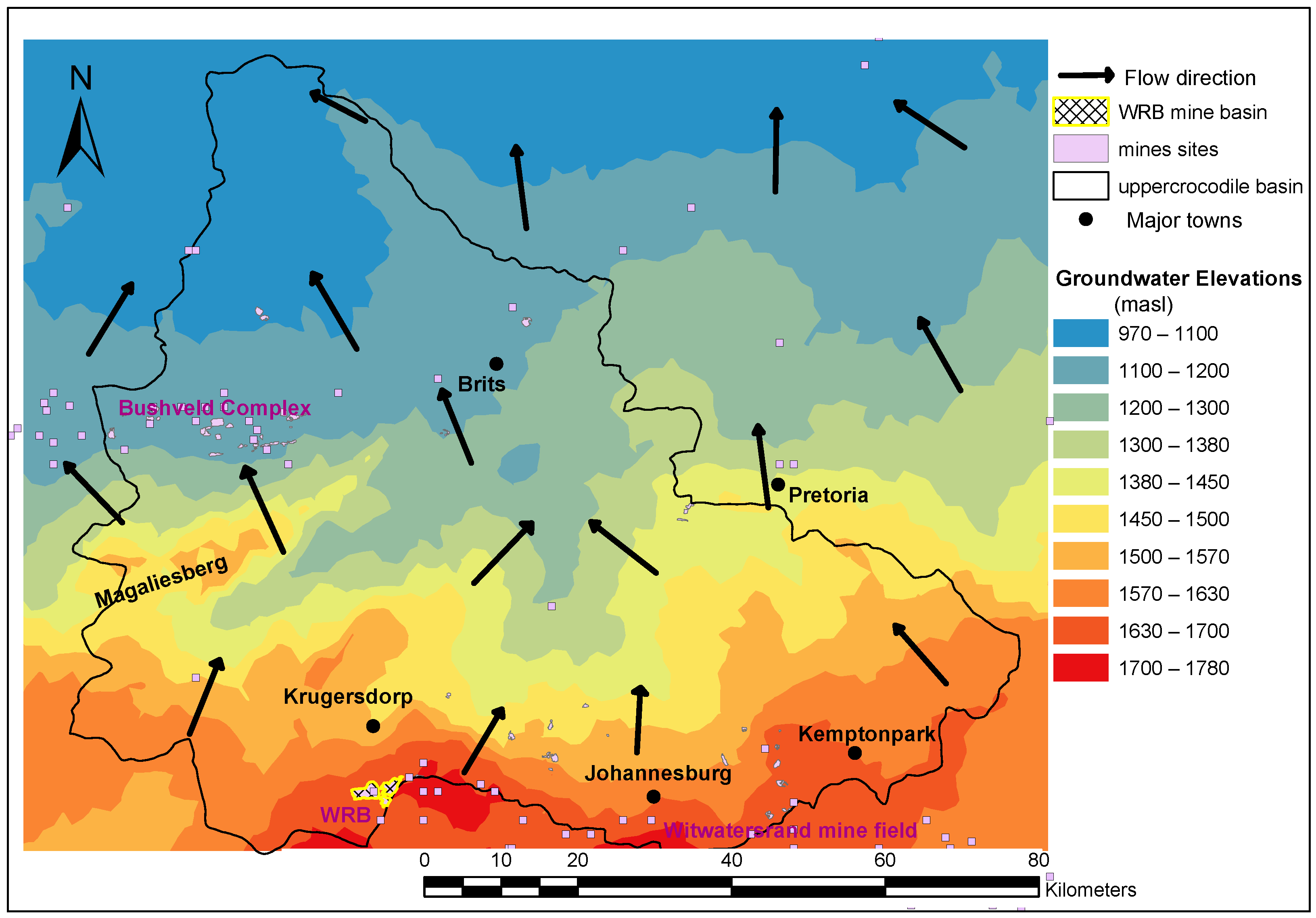
The catchment is underlain by fractured/weathered hard rock aquifers consisting of the Transvaal Formation (quartzite, shale, and dolomite) and rocks from the Bushveld Igneous Complex (gabbro, norite, and granite) [19]. The Bushveld Igneous Complex is one of the major geological features of this catchment, consisting of volcanic intrusive rock covering the area from north of the Magaliesburg and stretching eastward. The catchment also consists of sedimentary rock, with the quartsitic Magaliesberg Mountain Range being the prominent feature [23]. The Karst dolomitic formations are found in a band running east–west between Rietvlei Dam and Krugersdorp. The formation is comprised of chert-rich dolomite, with consequent high-water storage capacity. The northern part of the catchment is mostly underlain by intergranular/fractured aquifer [23]. Depth to groundwater table ranges from 12 m in the northern side to 33 m in the south-western side of the basin. The groundwater elevation varies significantly in the southern part towards the Magaliesberg mountain range (1780–1300 masl) and less variably in the northern side (Figure 2). Generally, groundwater in the basin flows in the south–north direction (Figure 2).
Groundwater resources in the catchment are generally highly developed and are utilised for demand supply and economical activities. The most productive aquifers are the Gauteng dolomites lying from east to west in the southern part of the basin and comprise two compartments, Bapsfontein and Steenkoppies in the eastern and western part, respectively. These compartments are extensively used for irrigation and contribute to the public water supply of towns including major municipalities, Johannesburg, and Tshwane (also known as Pretoria). One of the largest and best-known natural springs in the country—the “Maloney’s Eye”—is also found in the basin. There are several springs running in the basin (e.g., Rietvlei, Sterkfontein, Grootfontein, Upper and Lower Pretoria Fountain) and feeding-in rivers and streams in the basin.
Although very little has been done in quantifying the quality of groundwater in the catchment, the quality of most aquifer compartments is taken to be fair [8,24]. The most serious groundwater quality problem reported is an observed lower level of pH in the West Rand basin (WRB) [8,22,25]. Further, levels of sulphate and other salts have been reported to rise significantly as seen in Table 1. More significant is the potential impacts of contaminated water flowing from the WRB mine basin through the Krugersdorp game reserve all the way into the Cradle of Humankind World Heritage Site in Skeerpoort [8,21].
3.2. Methods
This research was carried out in a GIS environment using the geostatistical wizard to reveal the spatial variation of the groundwater quality based on nine water quality parameter measurements. Groundwater quality data from 90 boreholes monitored by the Department of Water Affairs (DWA)—South Africa scattered all over the catchment (see Figure 1) were analysed. Intervals of groundwater sampling varied significantly within the basin; some boreholes were sampled quarterly (once in every three months), especially in the south-western part of the basin. Most of the boreholes in the northern part had two data values a year. Annual averages of nine groundwater quality parameters, including , , , , , , DMS, , and were considered in the computation of the groundwater quality index (GQI). Since the monitoring network within the study basin is very poor, with most of the monitoring boreholes concentrated in a few parts of the catchment (see Figure 1), data exploratory analysis was performed. The exploratory data analysis was limited to determining variable distribution patterns and fitting the theoretical semivariogram. Explorations in the distribution of variables were carried out using histogram and normal QQ plots to determine whether the analysed data followed a normal distribution. In the case of non-normal distribution, a log transformation was performed. The output cell size for the rasters was set to 0.44 km.
3.2.1. Development of Groundwater Quality Index
The formulation of the GQI was accomplished following procedures outlined by [15]. The groundwater quality data from the boreholes were computed into a corresponding index rating value related to groundwater quality. The measured concentration, , was related to the universal norm—its permissible WHO standard value [26], X (Table 1)—using a normalized difference index [15] (Equation (1)).
where C is the contamination index value. The contamination index (C) obtained from Equation (1) was then rated between 1 and 10 to generate the quality index. The rating 1 indicates minimum impact on groundwater quality, while the rating 10 indicates maximum impact. Using the polynomial function (Equation (2)), the minimum contamination index level was set equal to 1, the median level (0) was set equal to 5, and the maximum level (1) was set equal to 10. Thus, the rank of the contamination level (r) in every point was given as:
The groundwater quality index was then calculated using the rank value and parameter weighting as follows:
where r is the rank value (1–10), w is the relative weight of the parameter which corresponds to the weight of “mean” rating value (r) of each parameter, and n is the water quality parameters involved in the computation. In the case of parameters which inflict potential health risk (e.g., nitrate), the mean r + 2 (for r < 8) is used; N is the total number of parameters used in the analysis. The weight factor (w) assigned to each parameter represents its relative importance to groundwater quality, and it corresponds to the mean ranking value. Parameters that inflict higher impact over groundwater quality (high mean rate) are similarly assumed to be more important in evaluating the overall groundwater quality. In this way, the impact of an individual parameter is greatly reduced, and the index computation is not bounded to a certain parameter.
For simplicity of presentation, the GQI can be projected such that high index values close to 100 reflect high water quality and index values close to 1 indicate low water quality (see Equation (4)). This approach has been applied by [15] in calculating GQI and [27] in the estimation of an index for aquifer water quality (IAWQ).
3.2.2. Spatial Analysis of the GQI with GIS
In conducting the geostatistical analysis, the “kriging” interpolation technique within the geostatistical analyst extension in ArcMap 10.1 software was used for data analysis and prediction. The spatial analyses were carried out using a calculated index from all points to determine the GQI for the distribution area. Unlike other point interpolation methods (nearest neighbour or inverse distance weighted), kriging is built on a statistical method. The kriging method performs a weighted averaging on point values, where the output estimates equal the sum of product of point values and weights divided by the sum of weights. Its main advantage is not only its ability to provide an estimate of the value of spatially distributed variables, but also an assessment of the probable error associated with these estimates [17]. Kriging methods are specifically designed to model spatial variability and offer an effective way to estimate contaminant concentrations in un-sampled areas [17,18]. Ordinary kriging is a linear interpolator that predicts a value at a point of a region of a known variogram without prior knowledge of the distribution mean. Ordinary kriging not only assumes the mean to be constant over the entire domain, it is also assumed to be constant in the local neighbourhood of each estimation point [16,28]. The ordinary kriging formula is given as follows: [28]
where Z(u) is the estimated value at estimation location u, Z() is the measured value at the location (i) and is the unknown weight for the measured value at the location (i). The unknown weight () depends on the distance to the location of the prediction and the spatial relationships among the measured parameters. The best model among a number of models provided in the geostatistical wizard was determined by fitting an experimental semivariogram to observed data. The best-fitting model was selected based on two criteria: the root mean square standardized error (RMSSE) and the mean error (ME). The closer the RMSSE is to 1, the better the predictive power of the model [12], while the mean error must be close to 0. The spatial dependency of the water quality parameters involved was determined using the nugget-to-sill ratio cited in [12]. The spatial structure is considered strong when the ratio is <0.25, moderate 0.25–0.75, and weak when >0.75 [12].
3.2.3. Optimal GQI
For multiple regression models like the one used in this study, the multicollinearity (also collinearity) phenomenon is common. The likelihood that two or more predictor variables in a regression model can be highly correlated such that one can be linearly predicted from the others with a substantial degree of accuracy is higher. This is moreso in this case, since most of the major chemical constituents in groundwater are spatially correlated. The use of all parameters in the estimation of GQI may result in duplication, and increases the probability of misjudgement. To address this concern, the use of optimum index factor (OIF) to select the best combination of groundwater quality parameters for the generation of GQI was adopted (see Equation (6)). The OIF was developed to select the optimum combination of three bands in a satellite image to create a color composite. This was proven useful in other fields (e.g, groundwater and soil) [15,29]. The optimum combination of parameters out of all possible three-parameter combinations is the one with the highest amount of “information” (highest sum of standard deviations), with the least amount of duplication (lowest correlation among band pairs). OIF is said to increase the spatial variability of the model [15].
where i, j, and k are any three parameters, SD is the standard deviation, and Corr is the correlation coefficient between parameters.
3.2.4. Temporal Variation of Groundwater Quality
Variation analysis in seeking to understand the stability of the groundwater quality within the basin was performed. The Coefficient of Variation (CV) was used to compare the GQI for 2006 and 2011 by estimating the degree of variation of groundwater quality over a 5-year period. The degree of variation was used to delineate regions underlain by relatively stable groundwater quality. This may work as a hand tool for screening possible new pollutant sources in the area or to evaluate the aquifer response to proposed remediation measures. The variation of groundwater quality was estimated as the ratio of the standard deviation to the mean of the two GQIs at different measured positions. A variation map was generated from the point data using a geostatistical interpolation technique in a GIS-environment.
4. Results
4.1. Exploratory Data Analysis
Data used in determination of the GQI were examined to determine the distribution of each parameter. The distribution patterns (Table 2) had the skewness of 1.08 and 0.8 for 2006 and 2011 data, respectively. For normal distributions, the skewness should lie between –1 and 1, while the mean should compare well with median [12]. Since the skewness value obtained for 2006 was slightly higher than 1 as suggested by [12] for a normal distributed pattern, data were log-transformed to allow for better model fitting. The 2011 data had a skewness within the suggested range, however, the mean and median had a significant difference. Therefore, log-transformation was also applied to 2011 data.
4.2. Semivariogram Analysis
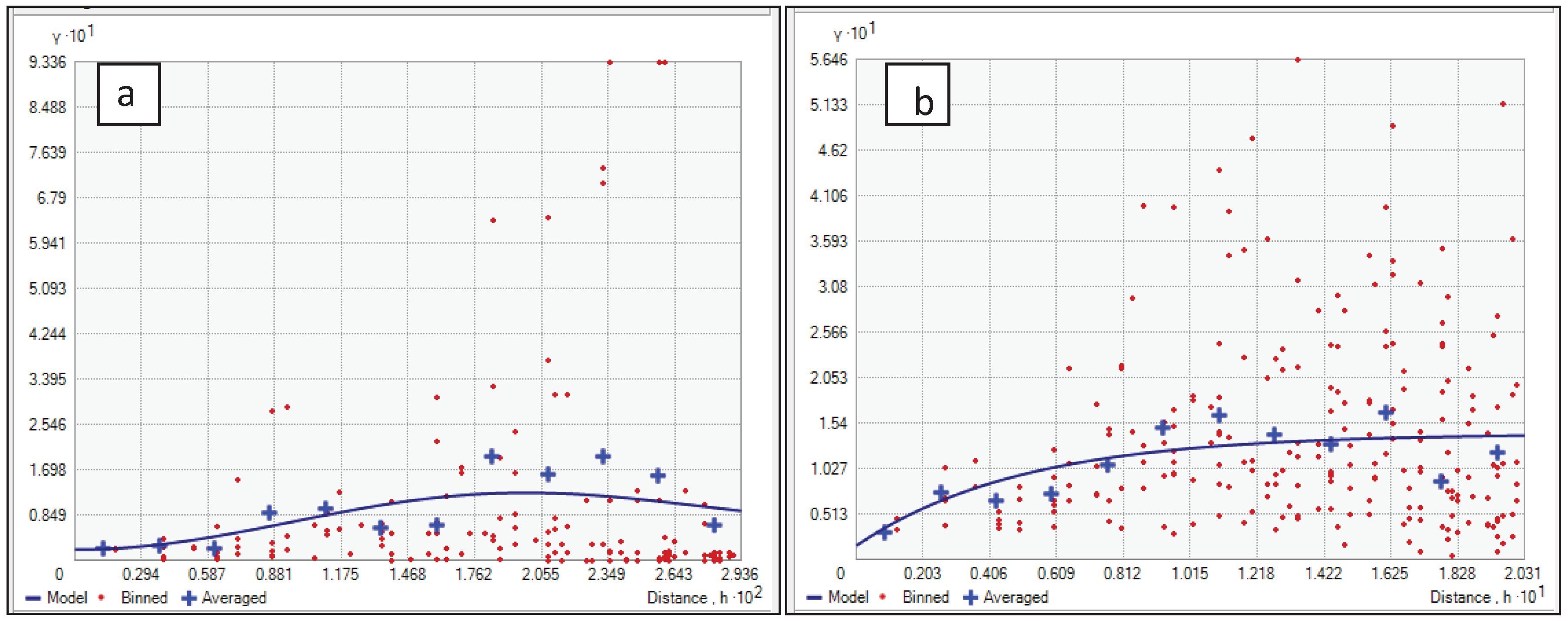
To determine the best fit model for the ordinary kriging, semivariograms of stable, Gaussian, exponential, and J-Bessel models—which are among the widely available models—were compared. A summary of the model comparison is presented in Table 3. The comparison results indicated the best fit model for 2006 data to be a J-Bessel semivariogram (Figure 4a), while an exponential model best fit the 2011 data (Figure 4b).
The nugget/sill ratio (Table 3) indicated a strong spatial dependency in both years. This was expected due to the existing relationship between water quality parameters. Considering the complexity of relationships between water quality parameters, it is difficult to draw a clear conclusion directly from the nugget/sill ratio of which parameters are more dependent on others. Further analysis was performed using SPSS to address the spatial dependency between the parameters.
4.3. Development of the GQI
Table 4 give statistics (using rank values) of nine parameters used in the creation of a GQI map. Parameters such as , dissolved mineral solids, , and had higher mean rank values, which may tend to dictate the spatial pattern of groundwater quality. In order to understand the contribution of each parameter in the deterioration of the groundwater quality in different parts of the basin, percentage increase in concentration for each parameter within 5 years was calculated and plotted (Figure 5). Results indicated a significant increase in sulphate concentration in the south-western part of the basin (Figure 5). Other salts, such as calcium, magnesium, and sodium were also noticed to increase. In the northern part, higher elevation of calcium (Ca) in relation to other parameters was observed. Generally, an increasing trend was observed in most areas for most of the parameters (Figure 5).
The Spearman rank-order correlation analysis was applied to non-normally distributed water quality data to detect spatial similarity and dissimilarity on each other. The results (Table 5) reveal positive correlation for all parameters, except for the weak negative correlation between and , and and (correlation coefficients of −0.008 and −0.045, respectively). showed a significant positive correlation with most of the parameters, which indicated its influence on other indicators. The strongest correlation was observed between and DMS (correlation coefficient of 1), indicating linear predictability between these two parameters.
Following the spatial similarity observed using the nugget/sill ratio (Table 3) and Spearman correlation analysis (Table 5), the determination of optimal parameters for the prediction of GQI was necessary. Using the OIF approach, combination of , , and had the highest index factor and was used for the prediction of the optimal GQI. Generally, the optimal GQI (Figure 6b) reveals a pattern of spatial variability of groundwater quality in the study area similar to that of the ordinary GQI (Figure 6a). The highest index values of the water quality for optimal GQI compared well with the ordinary at 84.6 and 84.4, respectively. However, there was a substantial difference in the standard deviation, indicating higher spatial variability in the optimal GQI (SD = 22.13) than the ordinary GQI (SD = 12.98). Therefore, with this observation, the optimum index is more suitable for the assessment of spatial groundwater quality than the use of absolute parameters.
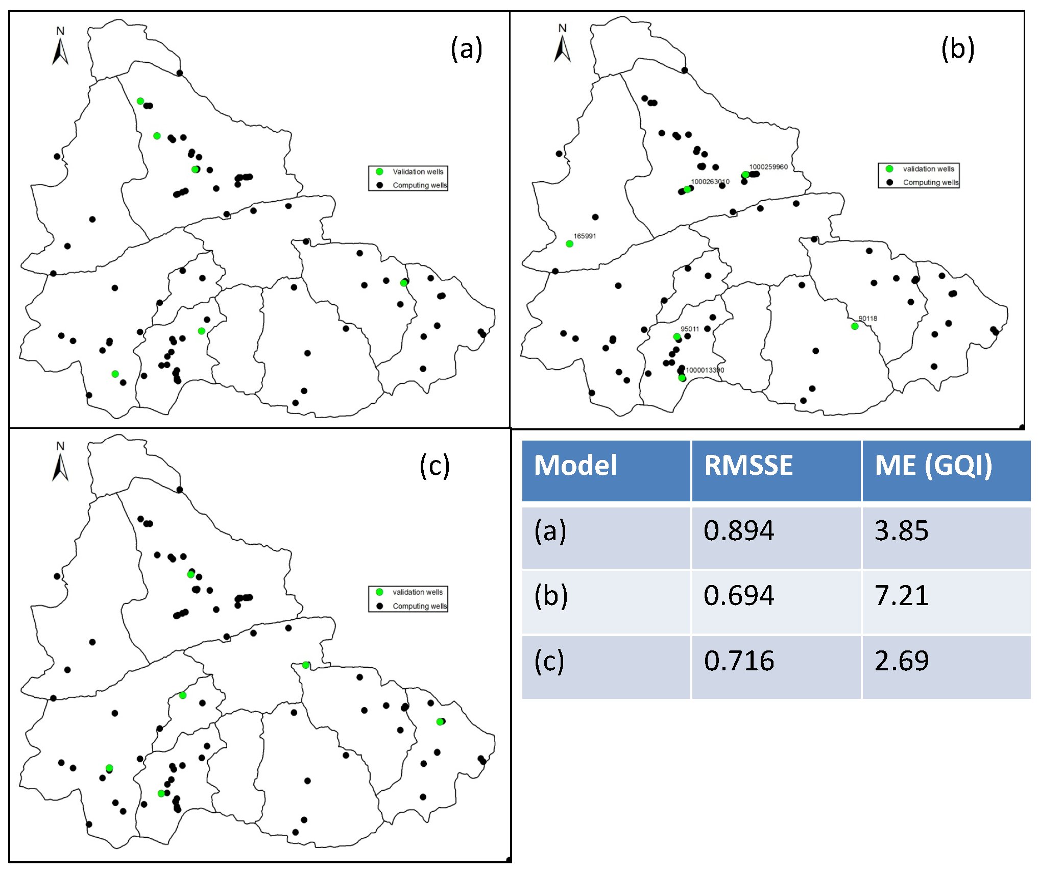
4.4. Model Validation
Model validation was performed to evaluate the credibility of the prediction model. Six groundwater quality sampling points were randomly removed in the calculation of the GQI and used to validate the result of the prediction model. The model performance was evaluated using two criteria: the root mean square standardized error (RMSSE) and the mean error (ME). Three series of six sampling points were tested, and their results analysed (Figure 7). The model gave a fair fit with RMSSE between 0.894 and 0.694, and ME of GQI between 2.69 and 7.21 (Figure 7). The results demonstrated that the model can reasonably estimate the spatial variation of groundwater quality using point data.
4.5. Variation Analysis
Figure 8a,b show the spatial variation of groundwater quality in years 2006 and 2011, respectively. The groundwater quality of the Upper Crocodile basin is generally fair, with predicted mean GQI of 72 (at max = 84.4) and 67 (max = 82.6) in 2006 and 2011, respectively. Five classes (see Figure 8) were used to classify the groundwater quality in the basin. Groundwater with GQI 30 was considered to be of poor quality, 50–70 of moderate quality, 70–80 of acceptable quality, and greater than 80 as water with good quality. A large area of the catchment falls between GQI of 50 and 80, indicating fair water quality.
Comparing Figure 8a,b reveals a deterioration of groundwater quality from measurements taken in 2006 and five years later. Changes are observed in the southern part of the catchment, which is bordered by the richest mineral deposit of Witwatersrand characterised by a large number of defunct old mines. The pollution observed in Krugersdorp and part of Johannesburg may be associated with the flow of groundwater through these old mines field. The most serious is the one in Krugersdorp, emanating from the now decanting mines in the WRB. This is evidenced by the higher level of (4593 mg/L) recorded at Randfontein estates gold mine and the significant elevation of sulphate and other salts as seen in Figure 5. The dispersion of pollutant plume is observed to follow the general groundwater flow direction (south–north). From Figure 8a, it can be perceived that the pollution plume is narrow and close to the boundary (in the WRB old gold mine shafts), while in Figure 8b it is wide-spread downstream, suggesting that pollution emanates from the upstream and spreads downstream towards the north.
Groundwater quality deterioration is also found in the northern part of the basin, characterised mostly by fractured aquifer. These aquifers are prone to contamination due to their ease of percolation. Water quality deterioration is due to elevated concentration levels of salts (, , and ) and major anions ( and ) (Figure 5) that can be associated with the intensive agricultural activities taking place in the area and mining activities in the Bushveld belt. This was previously reported in [24], where mines were considered as a salt sink, increasing salinity levels in both surface and groundwater resources. On the other hand, the south-eastern part of the catchment had a slight change in water quality. The change may be linked to the densely-populated towns in this part of the basin, including the south-western parts of Pretoria, Midrand, and Kempton park, which increases the chance of anthropogenic contamination.
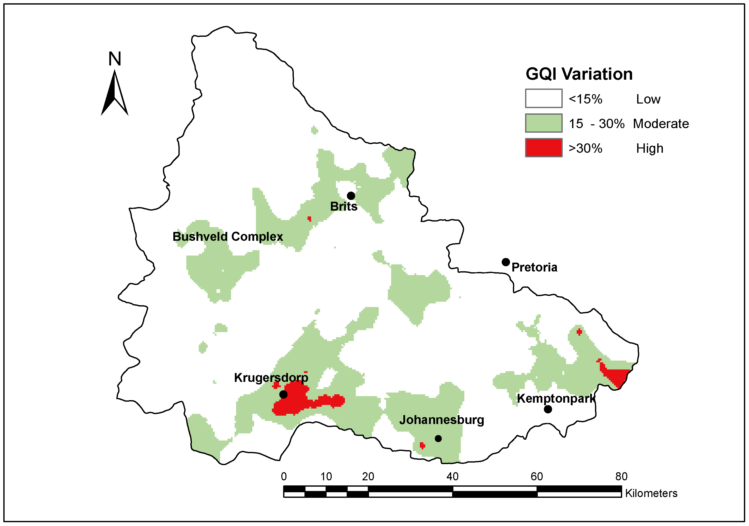
Figure 9 shows the temporal variation of groundwater quality in the catchment. As expected, the quality of groundwater is variable along the Bushveld complex, and the southern part of the catchment bordering the Witwatersrand gold mine field (coefficient of variation, CV: 15–30%), which attributes the variation to mining activities in the areas. The impact of decanting mines in Krugersdorp is significant, and to a large extent has made the groundwater quality in the area most variable (CV > 30%).
5. Summary and Conclusions
The importance of groundwater in supplying demand has increased drastically over the past years due to escalating challenges facing surface water resources. With the increasing demand for groundwater utilization, the quality of water in different aquifers becomes the only limiting factor. Assessment of groundwater quality in the aquifer has therefore become vital to ensure the availability of safe water for human uses and ecosystem support. However, describing the spatial variability of the overall water quality condition is difficult due to the lack of an effective monitoring system and the wide range of possible water quality indicators (chemical, physical, and biological) to be considered. This study makes use of geostatistical tools to determine the spatial distribution of groundwater quality index in a mining basin by combining nine parameters (, , , , , , DMS, , and ). The best fit model is a semivariogram of J-Bessel for 2006 and exponential for 2011 data. The model indicated strong spatial dependency in both periods. Parameter similarities were also observed in the correlation analysis. Using OIF, , , and were found to be the optimal parameters for the prediction of the GQI.
The groundwater quality of the Upper Crocodile basin is generally fair, with average GQI of 72 and 67 in 2006 and 2011, respectively. Generally, the quality of groundwater resources in most parts of the Upper Crocodile catchment is mostly acceptable and satisfactory. However, unsuitable water quality (GQI < 30%) was found in mining areas of Krugersdorp and in the northern part of the basin. The variation analysis between the two periods indicated a declining trend in water quality, which calls for continued monitoring of water quality in the areas for effective management.
The proposed approach was able to relatively estimate the spatial variation of the groundwater quality from available data. However, confidence of the estimation depends on the quality of data used and the spatial distribution of observation points in the area. Therefore, based on the problem at hand, local measurement of water quality indicators may be required for more accurate estimation.
Acknowledgments
This research was funded by Tshwane University of Technology.
Author Contributions
Augustina Alexander and Julius Ndambuki conceived the research idea; Augustina Alexander developed the method and did the analysis while Julius Ndambuki, Ramadhani Salim and Alex Manda providing review and comments. All the authors were engaged in the final manuscript preparation and agreed to the publication of this paper.
Conflicts of Interest
The authors declare no conflict of interest.
Abbreviations
The following abbreviations are used in this manuscript:
| DMS | Dissolved Mineral Solids |
| GQI | Groundwater Quality Index |
| GIS | Geographical Information System |
| CV | Coefficient of Variation |
| OIF | Optimal Index Factor |
| WRB | WestRand Basin |
References
- Department of Water Affairs (DWA). Classification of Significant Water Resources in the Mokolo and Matlabas Catchments: Limpopo Water Management Area (WMA) and Crocodile (West) and Marico WMA WP10506: Information Analysis Report: Crocodile West and Marico WMA; Report No: RDM/WMA1,3/00/CON/CLA/0112A; Department of Water Affairs: Pretoria, South Africa, 2012. [Google Scholar]
- Ashton, P.J.; Love, D.; Mahachi, H.; Dirks, P. An Overview of the Impact of Mining and Mineral Processing Operations on Water Resources and Water Quality in the Zambezi, Limpopo and Olifants Catchments in Southern Africa; Contract Report to the Mining, Minerals and Sustainable Development (Southern Africa) Project, by CSIR-Environmentek, Pretoria and Geology Department, University of Zimbabwe-Harare, Report No. ENV-PC; MMSD: Birnam Park, South Africa, 2001; Volume 42. [Google Scholar]
- McCartney, M.P.; Yawson, D.K.; Magagula, T.F.; Seshoka, J. Hydrology and Water Resources Development in the Olifants River Catchment; IWMI: Battaramulla, Sri Lanka, 2004; Volume 76. [Google Scholar]
- Daniel, M.; Anton, E. Water Resources of the SADC: Demands, Dependencies and Governance Responses; Institute for Global Dialogue (IGD) and Open Society Initiative for Southern Africa (OSISA) Workshop on Natural Resource Dependence in Southern Africa: Towards Equitable, Accountable and Sustainable Use; Institute for Global Dialogues and Open Society Initiative for Southern Africa: Pretoria, South Africa, 2007. [Google Scholar]
- Fornes, J.M.; la Hera, A.; Llamas, M.R. The silent revolution in groundwater intensive use and its influence in Spain. Water Policy 2005, 7, 253–268. [Google Scholar]
- Stamatis, G.; Voudouris, K.; Karefilakis, F. Groundwater pollution by heavy metals in historical mining area of Lavrio, Attica, Greece. Water Air Soil Pollut. 2001, 128, 61–83. [Google Scholar] [CrossRef]
- Meenal, M.; Eldho, T. Simulation-optimization model for groundwater contamination remediation using meshfree point collocation method and particle swarm optimization. Sadhana 2012, 37, 351–369. [Google Scholar] [CrossRef]
- Hobbs, P.J.; Cobbing, J. A Hydrogeological Assessment of Acid Mine Drainage Impacts in The West Rand Basin, Gauteng Province; Report : CSIR/NRE/WR/ER/2007/0097/C; Council for Scientific and Industrial Research (CSIR): Pretoria, South Africa, 2007. [Google Scholar]
- Naicker, K.; Cukrowska, E.; McCarthy, T. Acid mine drainage arising from gold mining activity in Johannesburg, South Africa and environs. Environ. Pollut. 2003, 122, 29–40. [Google Scholar] [CrossRef]
- Prakash, O.; Datta, B. Optimal monitoring network design for efficient identification of unknown groundwater pollution sources. Int. J. GEOMATE 2014, 6, 785–790. [Google Scholar] [CrossRef]
- Rebolledo, B.; Gil, A.; Flotats, X.; Sánchez, J.A. Assessment of groundwater vulnerability to nitrates from agricultural sources using a GIS-compatible logic multi-criteria model. J. Environ. Manag. 2016, 171, 70–80. [Google Scholar] [CrossRef] [PubMed]
- Gyamfi, C.; Ndambuki, J.; Diabene, P.; Kifanyi, G.; Githuku, C.; Alexander, A. Using GIS for spatial exploratory analysis of borehole data: A firsthand approach towards groundwater development. J. Sci. Technol. 2016, 36, 38–48. [Google Scholar] [CrossRef]
- Kourgialas, N.; Karatzas, G.; Koubouris, G.C. GIS policy approach for assessing the effect of fertilizers on the quality of drinking and irrigation water and wellhead protection zones (Crete, Greece). J. Environ. Manag. 2016, 189, 150–159. [Google Scholar] [CrossRef] [PubMed]
- Nikaeen, M.; Shahryari, A.; Hajiannejad, M.; Saffari, H.; Kachuei, Z.M.; Hassanzadeh, A. Assessment of the physicochemical quality of drinking water resources in the central part of Iran. J. Environ. Health 2016, 78, 40. [Google Scholar] [PubMed]
- Babiker, I.S.; Mohamed, M.A.; Hiyama, T. Assessing groundwater quality using GIS. Water Resour. Manag. 2007, 21, 699–715. [Google Scholar] [CrossRef]
- Dindaroğlu, T. The use of the GIS Kriging technique to determine the spatial changes of natural radionuclide concentrations in soil and forest cover. J. Environ. Health Sci. Eng. 2014, 12, 130. [Google Scholar] [CrossRef] [PubMed]
- Kourgialas, N.N.; Karatzas, G.P. An integrated approach for the assessment of groundwater contamination risk/vulnerability using analytical and numerical tools within a GIS framework. Hydrol. Sci. J. 2015, 60, 111–132. [Google Scholar] [CrossRef]
- Dokou, Z.; Kourgialas, N.; Karatzas, G.P. Assessing groundwater quality in Greece based on spatial and temporal analysis. Environ. Monit. Assess. 2015, 187, 774. [Google Scholar] [CrossRef] [PubMed]
- Water Research Commission (WRC). Design of Surface-Groundwater Interaction Studies: Implementing Uncertainity Analysis in Water Resources Assessment and Planning; Project No: K5/2056; Water Research Commission: Pretoria, South Africa, 2011. [Google Scholar]
- Basson, M.S.; Rossouw, J.D. The Crocodile (West) Reconciliation Strategy—Version 1: The Development of Reconciliation Strategy for the Crocodile (West) Water Supply System; Report: P WMA 03/000/00/3608; Department of Water Affairs and Forestry: Pretoria, South Africa, 2008. [Google Scholar]
- Hobbs, P.J. Water Resources Status Report for the Period April 2013 to March 2014: Surface Water and Groundwater Resources Monitoring, Cradle For Humankind World Heritage Site, Gauteng Province, South Africa; Report No. CSIR/NRE/WR/IR/2014/0049/A; Council for Scientific and Industrial Research (CSIR): Pretoria, South Africa, 2014. [Google Scholar]
- McCarthy, T.S. The impact of acid mine drainage in South Africa. S. Afr. J. Sci. 2011, 107, 1–7. [Google Scholar] [CrossRef]
- Department of Water Affairs and Forestry (DWAF). Crocodile River (West) and Marico Water Management Area: Internal Strategic Perspective of the Crocodile River (West) Catchment; DWAF Report No. 03/000/00/0303; Goba Moahloli Keeve Steyn (Pty) Ltd./Tlou, Matji (Pty) Ltd./Golder Associates (Pty) Ltd.: Johannesburg, South Africa, 2004. [Google Scholar]
- River Health Programme (RHP). State-of-Rivers Report: Monitoring and Managing the Ecological State of Rivers in the Crocodile (West) Marico Water Management Area; State-of-Rivers Reports Number 9; River Health Programme: Pretoria, South Africa, 2005; ISBN 0-620-34054-1. [Google Scholar]
- Oelofse, S. Emerging Issues Paper: Mine Water Pollution; Department of Environmental Affairs and Tourism (D EAT): Pretoria, South Africa, 2008; ISBN 978-0-9814178-5-1. [Google Scholar]
- World Health Organization (WHO). Guidelines for Drinking-Water Quality, 3 ed.; World Health Organization: Geneva, Switzerland, 2004; Volume 1. [Google Scholar]
- Melloul, A.J.; Collin, M. A proposed index for aquifer water-quality assessment: The case of Israel’s Sharon region. J. Environ. Manag. 1998, 54, 131–142. [Google Scholar] [CrossRef]
- Bohling, G. Introduction to Geostatistics and Variogram Analysis; Kansas Geological Survey: Lawrence, KS, USA, 2005; pp. 1–20. [Google Scholar]
- Kienast-Brown, S.; Boettinger, J. Applying the Optimum Index Factor to Multiple Data Types in Soil Survey. In Digital Soil Mapping: Bridging Research, Environmental Application, and Operation; Springer: Dordrecht, The Netherlands, 2010; pp. 385–398. [Google Scholar]
Figure 1.
Study area and borehole locations.
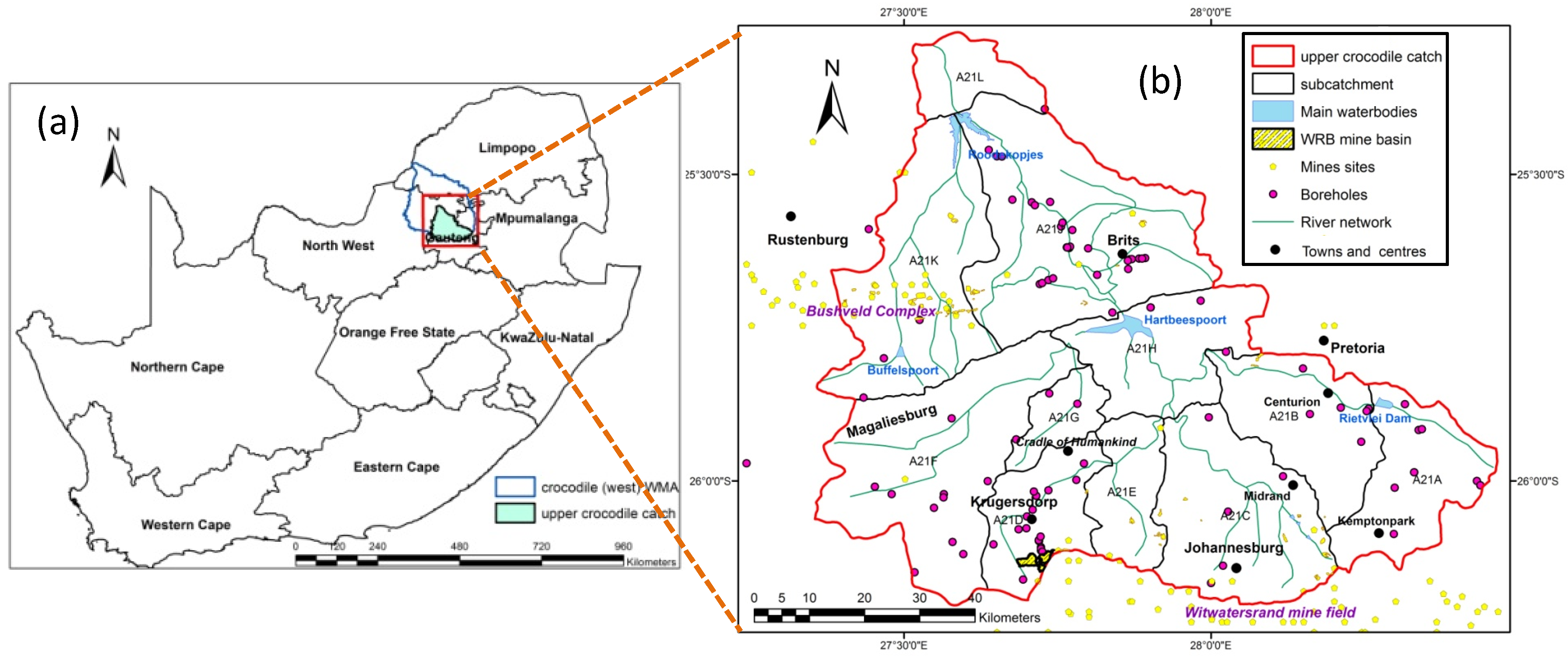
Figure 2.
Groundwater level and flow direction in the Upper Crocodile Catchment.

Figure 3.
Fitted log-normal distribution for (a) 2006 data (b) 2011 data.
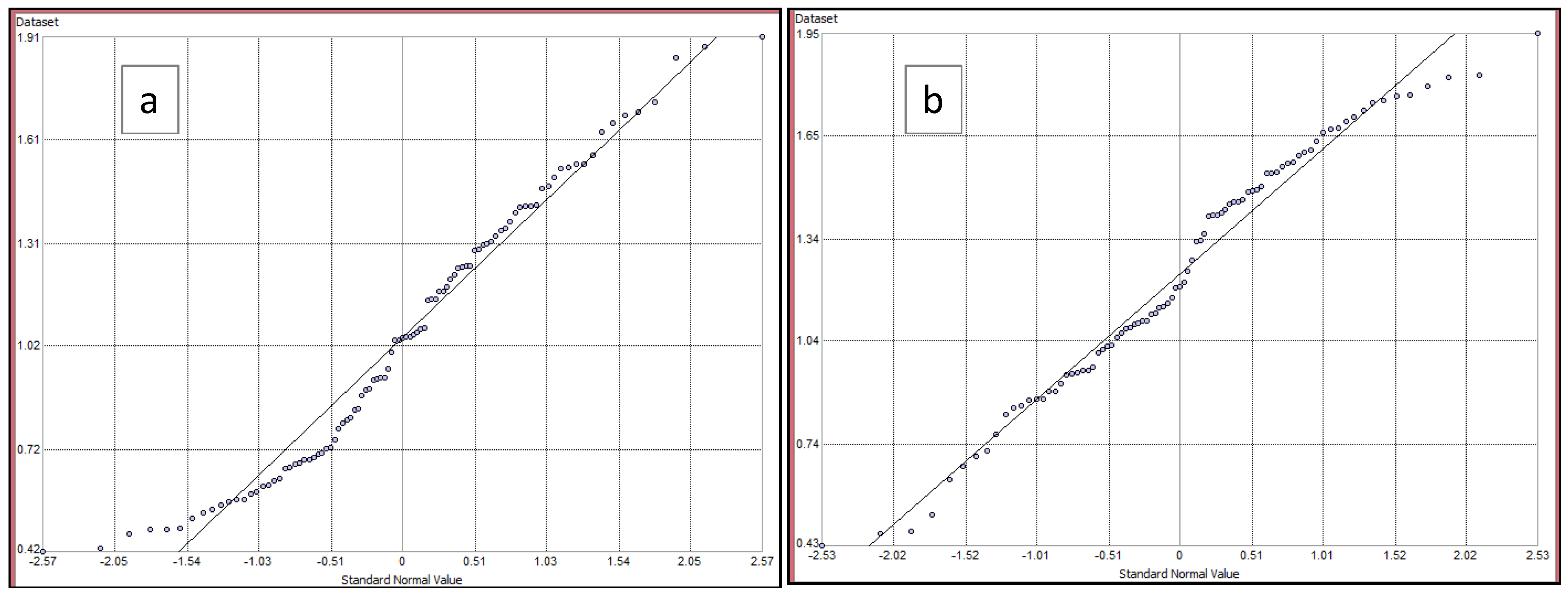
Figure 4.
Fitted log-normal distribution for (a) 2006 data (b) 2011 data.

Figure 5.
Groundwater quality parameter increase between 2006 and 2011.
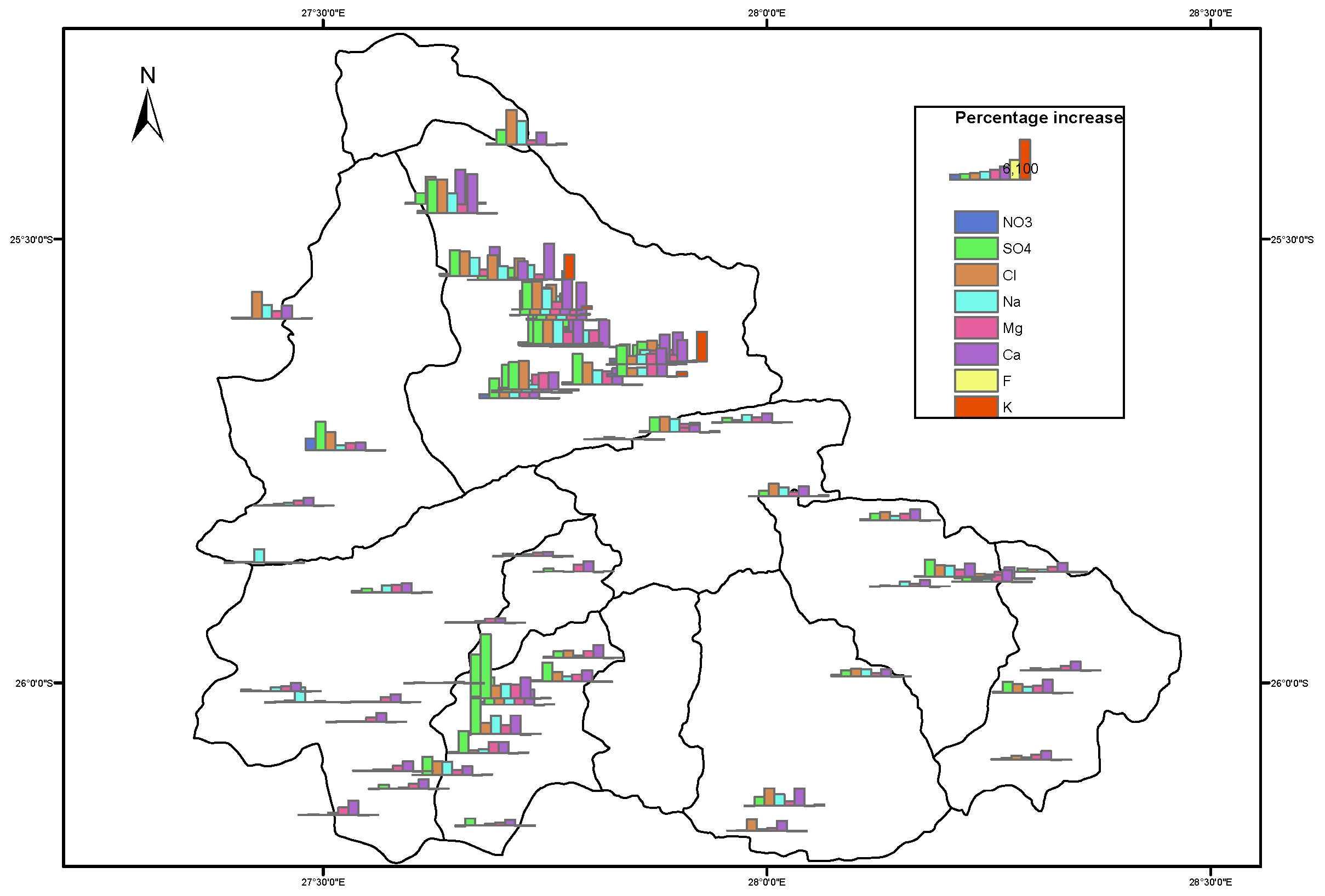
Figure 6.
(a) Groundwater quality index computed using all nine water quality parameters; (b) Optimal-GQI computed using three parameters only (, , and ).
Figure 6.
(a) Groundwater quality index computed using all nine water quality parameters; (b) Optimal-GQI computed using three parameters only (, , and ).
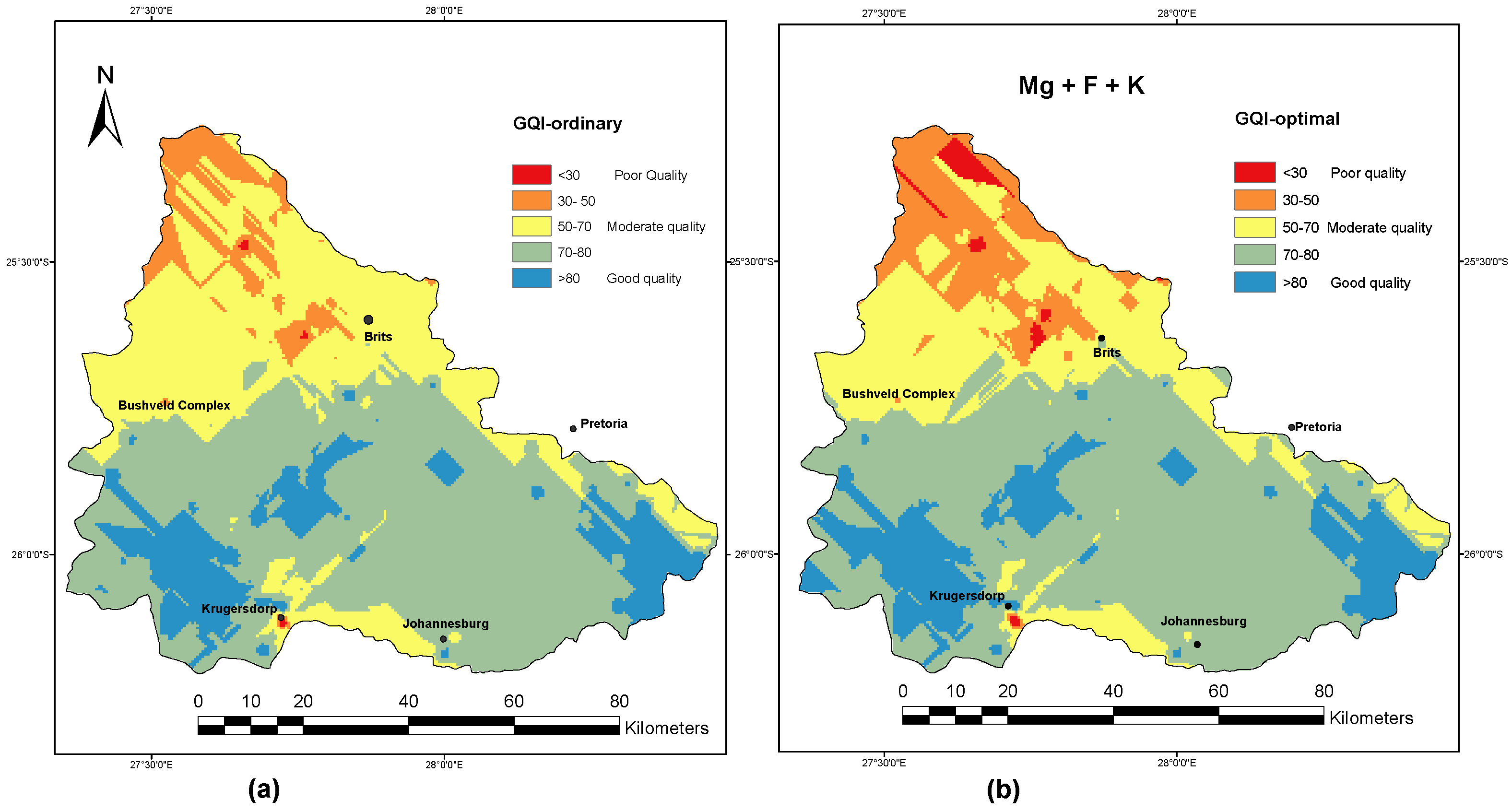
Figure 7.
Results of model validation.

Figure 8.
Groundwater quality index of the Upper Crocodile catchment (a) For 2006; (b) For 2011.
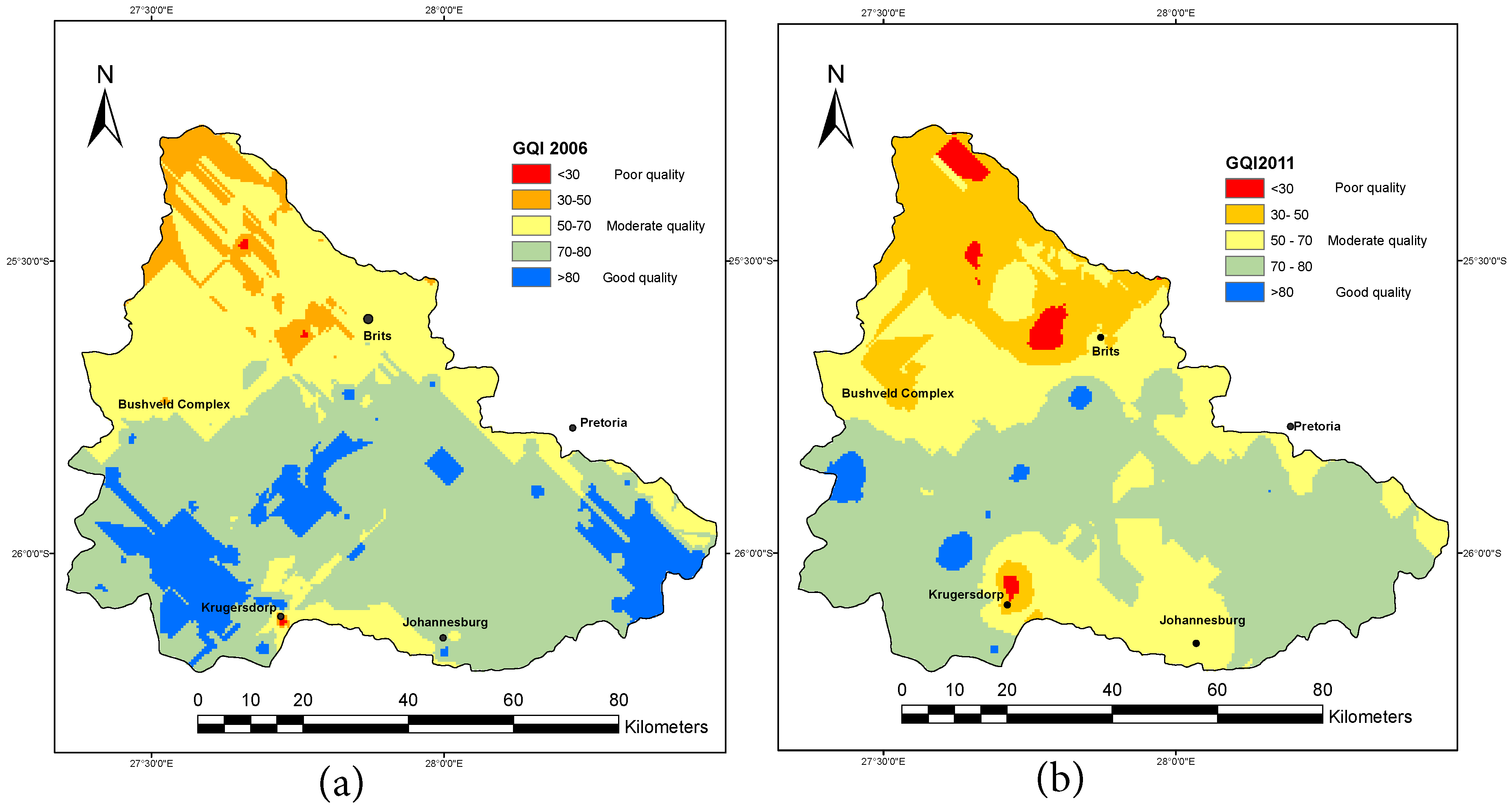
Figure 9.
Variation of groundwater quality between 2006 and 2011.

Table 1.
Upper-Crocodile groundwater quality data and recommended permissible limits (in mg/L).
| Parameters | Minimun | Maximun | Mean | Std Dev | WHO Std |
|---|---|---|---|---|---|
| 0.02 | 283.55 | 8.52 | 30.20 | 45 * | |
| 2.00 | 4592.93 | 268.12 | 845.83 | 250 | |
| 1.50 | 1039.71 | 70.61 | 131.84 | 250 | |
| 1.00 | 410.07 | 54.24 | 76.66 | 200 | |
| 0.50 | 227.05 | 44.93 | 52.39 | 100 | |
| 1.10 | 499.56 | 70.65 | 99.42 | 200 | |
| DMS | 13.00 | 5488.82 | 733.59 | 1010.96 | 600 |
| 0.00 | 7.88 | 0.42 | 1.08 | 1.5 | |
| 0.00 | 46.78 | 3.24 | 6.15 | 10 |
* Stared threshold might inflict potential health risk [26]; 0 value indicates undetectable concentration.
Table 2.
Statistics on original and log-transformed data.
| 2006 | 2011 | |||||
|---|---|---|---|---|---|---|
| Mean | Median | Skewness | Mean | Median | Skewness | |
| Normal | 3.05 | 2.83 | 1.08 | 3.82 | 3.32 | 0.8 |
| Log | 1.038 | 1.039 | 0.27 | 2.23 | 2.2 | −0.17 |
Table 3.
Summary of the semivariogram model comparison.
| Stable | Gaussian | Exponential | J-Bessel | |||||
|---|---|---|---|---|---|---|---|---|
| 2006 | 2011 | 2006 | 2011 | 2006 | 2011 | 2006 | 2011 | |
| RMSSE | 0.81 | 0.85 | 0.81 | 0.83 | 0.79 | 0.90 | 0.92 | 0.86 |
| ME | 1.03 | 1.12 | 1.01 | 1.13 | 0.95 | 1.11 | 0.88 | 1.09 |
| Nugget | 0.02 | 0.02 | 0.02 | 0.04 | 0.03 | 0.02 | 0.03 | 0.04 |
| Sill | 0.14 | 0.14 | 0.14 | 0.14 | 0.11 | 0.14 | 0.10 | 0.12 |
| Nugget/sill ratio | 0.14 | 0.17 | 0.14 | 0.28 | 0.27 | 0.11 | 0.27 | 0.36 |
ME: mean error; RMSSE: root mean square standardized error.
Table 4.
Summary of the parameter index value used in the prediction of groundwater quality index (GQI).
Table 4.
Summary of the parameter index value used in the prediction of groundwater quality index (GQI).
| Min | Max | Mean | Std Dev | |||||
|---|---|---|---|---|---|---|---|---|
| 2006 | 2011 | 2006 | 2011 | 2006 | 2011 | 2006 | 2011 | |
| 1.00 | 1.00 | 8.53 | 7.46 | 1.72 | 1.63 | 1.16 | 0.90 | |
| 1.06 | 1.04 | 9.44 | 8.86 | 2.68 | 2.92 | 2.12 | 2.08 | |
| 1.04 | 1.04 | 7.94 | 7.73 | 2.19 | 2.28 | 1.49 | 1.46 | |
| 1.03 | 1.02 | 6.61 | 6.46 | 2.26 | 2.37 | 1.37 | 1.27 | |
| 1.03 | 1.03 | 6.82 | 6.31 | 2.93 | 3.08 | 1.49 | 1.47 | |
| 1.04 | 1.04 | 7.02 | 6.95 | 2.59 | 2.84 | 1.29 | 1.40 | |
| DMS | 1.02 | 1.15 | 6.24 | 8.60 | 1.63 | 4.63 | 0.91 | 1.71 |
| 1.00 | 1.00 | 8.29 | 8.56 | 2.06 | 1.79 | 1.36 | 1.17 | |
| 1.00 | 1.00 | 8.12 | 8.95 | 2.31 | 2.71 | 1.52 | 1.50 | |
Table 5.
Correlation matrix of groundwater quality parameters.
| 1 | |||||||||
| 0.474 ** | 1 | ||||||||
| 0.464 ** | 0.776 ** | 1 | |||||||
| 0.382 ** | 0.758 ** | 0.836 ** | 1 | ||||||
| 0.446 ** | 0.702 ** | 0.480 ** | 0.427 ** | 1 | |||||
| 0.359 ** | 0.670 ** | 0.545 ** | 0.482 ** | 0.757 ** | 1 | ||||
| DMS | 0.464 ** | 0.776 ** | 1.0 ** | 0.826 ** | 0.450 ** | 0.545 ** | 1 | ||
| 0.109 | 0.109 | 0.354 ** | 0.427 ** | −0.045 | 0.130 | 0.354 ** | 1 | ||
| −0.008 | 0.255 ** | 0.251 ** | 0.401 ** | 0.055 | 0.146 | 0.261 ** | 0.162 | 1 | |
| Cl | Na | Mg | Ca | DMS | F | K |
** Correlation is significant at the 0.01 level (two-tailed).
© 2017 by the authors. Licensee MDPI, Basel, Switzerland. This article is an open access article distributed under the terms and conditions of the Creative Commons Attribution (CC BY) license (http://creativecommons.org/licenses/by/4.0/).
Share and Cite
MDPI and ACS Style
Alexander, A.C.; Ndambuki, J.; Salim, R.; Manda, A. Assessment of Spatial Variation of Groundwater Quality in a Mining Basin. Sustainability 2017, 9, 823. https://doi.org/10.3390/su9050823
AMA Style
Alexander AC, Ndambuki J, Salim R, Manda A. Assessment of Spatial Variation of Groundwater Quality in a Mining Basin. Sustainability. 2017; 9(5):823. https://doi.org/10.3390/su9050823
Chicago/Turabian StyleAlexander, Augustina Clara, Julius Ndambuki, Ramadhan Salim, and Alex Manda. 2017. "Assessment of Spatial Variation of Groundwater Quality in a Mining Basin" Sustainability 9, no. 5: 823. https://doi.org/10.3390/su9050823
Note that from the first issue of 2016, this journal uses article numbers instead of page numbers. See further details here.