Energy Efficiency Gain of Cellular Base Stations with Large-Scale Antenna Systems for Green Information and Communication Technology


School of Intelligent Mechatronics Engineering, Sejong University, Seoul 05006, Korea
Sustainability 2017, 9(7), 1123; https://doi.org/10.3390/su9071123
Submission received: 26 May 2017
/
Revised: 20 June 2017
/
Accepted: 22 June 2017
/
Published: 27 June 2017
(This article belongs to the Section Energy Sustainability)
Abstract
:Due to the ever-increasing data demand of end users, the number of information and communication technology (ICT)-related devices and equipment continues to increase. This induces large amounts of heat emissions, which can cause serious environmental pollution. In recent times, signal transmission systems such as cellular base stations (BSs) have been constructed everywhere and these emit a large carbon footprint. Large-scale antenna systems (LSASs) that use a large amount of transmission antennas to serve a limited number of users can increase energy efficiency (EE) of BSs based on the beamforming effect, and thus can be a promising candidate to reduce the carbon footprint of the ICT field. In this paper, we discuss the necessary schemes to realize LSASs and show the expected EE gain of the LSAS with enough practicality. There are many obstacles to realize the high EE LSAS, and even though several studies have shown separate schemes to increase the EE and/or throughput (TP) of LSASs, few have shown combinations of schemes, and presented how much EE gain can be achieved by the schemes in the overall system. Based on the analysis in this paper, we believe more detailed work for the realization of high energy efficient BSs with LSASs is possible because this paper shows the necessary schemes and the maximum achievable energy efficiency gain as a reference. Extensive analysis and simulation results show that with proper implementation of the power amplifier/RF module and a robust channel estimation scheme, LSASs with 600 transmitter (TX) antennas can achieve times more EE gain compared to the current systems, thereby resulting in significant reduction of carbon footprints.
1. Introduction
There is no doubt that information and communication technology (ICT) dramatically changes our life. There are various eco-friendly aspects of ICT, such as a reduction in paper consumption, reduced transportation/traffic, global environmental monitoring and control, smart building and teleworking, and so on [1]. There are also various negative environmental aspects, such as the heat emission generated from data transmission and processing, garbage from manufacturing, disposal of PCs and smart phones, and so on. The ICT industry’s greenhouse gas (GHG) emissions account for about of global GHG emissions, and this value is growing rapidly [2]. Reducing environmental pollution from ICT is very important to the sustainability of Earth.
Among various ICT related devices/equipment that cause a lot of environmental pollution, signal transmission systems such as a cellular base stations (BSs) are one of the most power hungry devices [3]. Currently, the amount of data transmission increases about ten times every five years [4,5], and thus the energy efficiency (EE) increase of BSs is a vital research topic. Designing an energy efficient BS is particularly difficult, because the amount of signal transmissions is drastically increases day by day. Large-scale antenna systems (LSASs) that use a large number of transmitter (TX) antennas and serve a limited number of users, have a high possibility to increase the EE of the BS, and this has already been shown in several parts of the existing literature [6,7,8,9,10,11,12,13].
In this paper, we show how to increase the EE of the BSs using technologies related to LSASs to reduce the carbon footprint. There are several important components that we should note in an LSAS. We overview each component of the LSAS and derive the expected EE gain from each component with an appropriate scheme. In current BS systems, the power amplifier (PA) consumes around 60∼80% of total power consumption [14,15]. Reducing PA power consumption is a main research topic for current signal transmission systems. One of the distinct characteristics of the LSAS is the possibility of low radiation power due to the beamforming effect. Moreover, because of a large number of TX antennas, the radiation power of each PA can be fairly small. Therefore, with LSASs, the status of PA power consumption could be different from current systems. Also, since an LSAS has a large number of TX antennas, each TX antenna needs to be connected to an RF component. The RF component typically consists of a digital-to-analog converter (DAC), mixer, and filter. Current BSs only use less than 10 TX antennas, so power consumption of RF components is not a problem because it is much less than the power consumption of the PA. However, in LSASs, the number of TX antennas can be hundreds or more, and thus reducing the power consumption of RF components could become a major research topic. Another component we can think of is baseband (BB) power consumption. Typically, BB power consumption is significantly less than PA and RF power consumption. However, BB processing is related to signal processing, and depending on the signal processing algorithm, it actually affects the spectral efficiency (SE) and/or data throughput (TP), which is a major parameter of EE. Also, BB processing is strongly related to the processing delay from high complexity signal manipulation, which should be prevented for low latency communication systems. Due to these reasons, BB processing is also considered as a factor that measures the EE of LSASs.
Assuming the PAs/RFs are implemented properly, the problem of reference signal (RS) overhead and the accuracy of channel estimation also should be discussed. Since RS numbers increase as the number of transmitter (TX) antennas or the number of users increases, reducing RS overhead is crucial for the realization of LSASs [16]. However, RS overhead reduction almost always accompanies channel estimation errors; thus we also show how the channel estimation error affects EE gain.
Even though several studies have shown separate schemes to increase the EE and/or throughput (TP) of LSASs, few have shown combinations of schemes, and presented how much EE gain can be achieved by the schemes in the overall system. Based on the analysis in this paper, we believe more detailed work for the realization of high energy efficient BSs with LSASs is possible because this paper shows the necessary schemes and the maximum achievable energy efficiency gain as a reference.
In our previous work [17], we presented an elegant power control scheme of future BS with LSAS. In the work, we proposed a future BS structure which includes several core components to improve EE. The structure is a kind of feedback system, and decision unit in the system gathers the related information and sends the information to the power control unit of the BS. Our current work is different from the previous work in several points. First, the main contribution of our previous work is proposing a new BS structure and related operation, while current work focuses on high level performance analysis of general LSAS; Second, we deals with various LSAS related obstacles and discussions which were not covered in our previous work, such as antenna size and form factor, channel estimation and reference signal (RS) overhead reduction issues; Third, there is little work to gather all the issues at once and show the expected performance gain from each perspective. In this work, we gathers all the related issues and combine all of them to show the expected performance gain.
The rest of this paper is organized as follows. In Section 2, we show the system model, including power consumption model, and also present precoding and effective signal-to-interference-noise ratio (SINR) here. In Section 3, we present the performance metric to show EE gain. In Section 4, we overview each component in LSASs, and present necessary schemes and related performance. In Section 5, we gather the results from Section 4 and present overall performance gain and related discussion. Lastly, the concluding remarks are given in Section 6.
2. System Model
To show the expected gain, a good system model should be defined first [17]. We consider a single isolated cell with one BS and K terminals/users. The BS has TX antennas, and each terminal has only one receiver (RX) antenna. The received signal vector at terminals can be represented as follows:
where is the received vector for K terminals, is the total TX power for downlink, is the small scale i.i.d. Rayleigh fading channel matrix between BS antennas and K terminals, is the TX signal vector, and is the additive white Gaussian noise (AWGN) vector at the terminals. As a simple rule of thumb, if , we say that the system is LSAS.
2.1. Precoding
Since we consider that in system is much larger than K, we need to map K message signals to each antenna; coincidently, the K message signals should less interfere each other at RXs. For this, the BS should transmit signals with some kind of precoding. Since is very large, linear precoding is tractable for real systems. It is well-known that zero-forcing (ZF) and regularized zero-forcing (RZF) are effective linear precoding techniques [18,19]. Also, in [6], T. Marzetta suggested even simpler precoding technique—matched filtering (MF) or conjugate transpose precoding. Note that MF precoding is only effective for LSASs, while ZF/RZF precoding is also useful for traditional multi-antenna systems. The relationship between the TX signal vector and the message signal vector can be expressed as follows:
where is the TX power normalization factor, and is the precoding matrix.
Then, (1) can be rewritten as:
All of the three precoding matrices are provided in Table 1, where the superscript denotes conjugate transpose, is the inverse operator, and is the an identity matrix. Note that RZF precoding can be the same as ZF and/or minimum mean square error precoding, if we choose .
As grows without bounds, the autocorrelation of channel vectors can be simplified as follows [6]:
Since the channel has a characteristic of mean zero and unit variance in a rich scattering environment, the autocorrelation of channel vectors become and the cross correlation of channel vectors becomes 0. Thus, simply we call (4) as the LSAS channel characteristic.
By applying (4), minimum mean square error and ZF can be simplified as
and it means that all representative linear precoding techniques show similar performance with an excessive number of TX antennas and limited number of RX antennas. It is well-known that ZF is near optimal in very high SNR regions. If we consider the complexity of nonlinear precoding techniques and high effective signal-to-interference plus noise ratio (SINR) of the LSAS, linear precoding would show enough performance with low complexity.
The normalization factor should be determined such that the total transmitted power becomes , and it is expressed as follows:
where stands for Frobenius norm.
Since and are independent, and we already chose the average power of the signal constellation in unity, can be represented as
Both ZF and the minimum mean square error precodings show very similar performance, even in the relatively practical number of large scale TX antennas (i.e., ). Due to this reason, we only consider MF and ZF as precoding techniques in this paper.
2.2. Power Consumption Model
Typical BS is composed of many power consumption components such as the power supply, cooling, baseband (BB), RF components, PA, and loss factors for DC-DC and feeding cable, etc. It is difficult to estimate how technology will evolve, and designing an exact model is out of the scope of this paper. In this paper, we define a sum power, , as a tractable power consumption model, which includes some of the important LSAS power consumption components that can be expressed as:
where is the power consumption of the PA and is the power consumption of circuits, which includes baseband power consumption, , and RF front-end power consumption, where is the RF front-end power consumption of each antenna. It is true that the PA is also a kind of circuit; however, since its operation is significantly important, and different from other circuits, we differentiate it from other circuits. Due to the beamforming effect, can decrease as increases, while increases as increases.
2.2.1. Power Amplifier Power Consumption Model
Current cellular standards use orthogonal frequency division multiplexing (OFDM) as a downlink transmission scheme, and there is no doubt that LSASs should use OFDM, because it has very high spectral efficiency and is robust against multipath fading. However, OFDM has a very high peak-to-average power ratio, which seriously reduces the PA efficiency [20]. If we assume 10 MHz bandwidth with 1024 subcarriers, the peak-to-average power ratio of an OFDM signal is higher than 11 dB with distortion probability or complementary cumulative distribution function. This means, without using digital pre-distorter or peak-to-average power ratio reduction schemes, we should choose Input-Back-Off of more than 11 dB for proper operation. We also assume that we use Class-B PAs, which have efficiency. The Class-B PA efficiency, , can be represented as follows [21,22]:
where p is the square-root of Input-Back-Off, . The simple relationship between and can be represented as:
2.2.2. Circuit Power Consumption Model
The power consumption of circuits except PA is divided as follows:
where is the power consumption of baseband (BB). Each parameter is a function of bandwidth, B, and we set B as 10 MHz. We only listed the components, which depend on . The can also be divided as follows:
where is the power consumption of the digital-to-analog converter (DAC), is the power consumption of the mixer, and is the power consumption of the TX filter [23]. The power consumption parameters for a low power TX are given in [24].
To get the , we use the following floating point operations per second (Glops), that was presented in [25,26,27,28]:
where is the length in the samples of the uplink sequences, and the description of each parameter is shown in Table 2. We took the parameters from [6] and from a current 3GPP LTE system [29]. The first part of (13) is to operate the FFT/IFFT operation, the second part is to implement precoding/decoding, the third part is to correlate the pilot signals with pilot sequences, and the last part is to contain the additional pseudo inverse for zero forcing (ZF) precoding.
The relationship between and can be represented as
where is the VLSI processing efficiency.
Let us assume for short guard interval and fast pilot correlation. When we use matched filtering (MF) precoding, the last part of (13) becomes zero, since MF precoding does not need to perform the pseudo inverse [25].
The success of an energy efficient LSAS depends on how small the is in . If occupies too much of , the increase of is of little help in increasing . That is, there is little room for to reduce sum power.
2.3. Effective SINR and Channel Gain
The symbol received by k-th user, , is given by
where is the channel vector for k-th user, and is the precoding vector for k-th user. The last term of (15) is inter-user interference (IUI). Note that an efficient method of channel estimation is very important to reduce the IUI. The effective SINR for user k, , can be represented as follows:
where is the noise power in the given bandwidth B.
In the ideal case that there is perfect channel state information at the TX and , the effective SINR can be simplified as:
where is the received signal power at RX, is the path loss component between TX and RX, and is the noise power in the given bandwidth, B. Here we can say that is the channel gain of the LSAS. It is obvious that if we increase the number of TX antennas or reduce the number of users, we can get better channel gain and/or effective SINR. However, it should be noted that MF precoding does not completely remove the IUI from a practical number of TX antennas. can be normalized to unity, and it is equivalent to the average path loss of 134 dB with 2 GHz carrier frequency [30].
3. Performance Metric for Measuring EE Gain
In this section, we present a performance metric for measuring EE gain. It is well-known that most signal transmission systems use SE or TP as a performance metric. However, EE could be more important than TP depending on the applications.
The justification of using the EE metric for LSASs is comes from Shannon’s channel capacity equation that is represented in AWGN channel as:
where is the signal-to-noise ratio (SNR) that shows how much signal power is received against noise power at RX. Equation (18) is plotted in Figure 1.
As observed, there are roughly two regions in the figure of channel capacity versus . In the region where is not sufficiently high, the channel capacity increases significantly as increases. We usually call this region as power limited region. The channel capacity logarithmically increases as increases. Due to this reason, once is high enough, even if continue to increase, it does little help to increase C. We call this region as bandwidth limited region. The bandwidth limited region is the region where is high enough that increasing is not particularly helpful in increasing C, while increasing B is very helpful. If we can increase the signal-to-noise ratio using a large amount of TX antennas, C goes to the bandwidth limited region, and thus we can reduce with little channel capacity loss. is tightly connected to the PA which is one of the most power hungry devices. This is the logic of using the EE metric.
The simplified channel capacity with beamforming effect can be represented as:
where is the beamforming factor from a large amount of TX antennas, which usually depends on the number of TX antennas, and is typically much larger than 1. With high , we can get room to reduce the TX power consumption, which consequently increases EE.
With this in mind, based on (17) and (19), the TP can be represented as follows:
where is the scaling factor to reflect guard interval, and reference signal overhead, etc. Although (20) has been used as a performance metric for a long time, the current form is not sufficient for some applications. The reason is that Equation (20) does not represent power consumption related performance. For example, based on (20), increasing TX power is always helpful, but that is not true on real systems. Equation (20) has had very high impact so far because the wireless TP has been always less than demand. Of course, there is still high TP demand, but today’s TP demand is a little bit different from the past. Moreover, environmental pollution from signal transmission systems is growing, and there is a consensus that reducing the carbon footprint has become much more important than previously.
For these reasons, the EE performance metric can be defined as the ratio of TP to power consumption:
Continuous increase of power consumption can increase EE only up to a certain point which is in the power limited region. Figure 2 shows the performance metric comparison and change of TP and EE.
4. EE Improvement Issues for Each Component
In this section, we provide EE improvement issues and schemes for each power related component. For the numerical simulations, we assume 1 ms coherence time, that means there are a total of 168 resource elements (12 frequency domains × 14 time domains) in two resource blocks of 3GPP LTE standard [29]. As a reference model, we use a multi-antenna system with 4 TX antennas and 4 users where each user has one antenna. For power consumption, we used 40 W radiation power with efficiency and 5 W RF power consumption. Relative TP and EE can then be defined as:
For analysis, we assume is successfully reduced to 6 W when , and PA efficiency is reduced to , since digital pre-distorter cannot be used. We also assume , since this is the minimum condition of the LSAS effect and it is natural that K can be increased as increases. Details are provided in each subsection.
4.1. Antenna Size
Since an LSAS is a system that integrates a large number of TX antennas in a limited space, the size and form factor of the installation site could be a problem. The antenna spacing should be at least , and in addition, since LSASs transmit different signals from each antenna, it is necessary to further increase the antenna spacing to reduce the correlation among the antennas. We present an example of antenna form factors in Figure 3. In Figure 3, we assume that we use 400 (20 × 20) antennas with antenna spacing ∼, and carrier frequencies of 2 GHz and 6 GHz. As observed, the required size of the LSAS is 1.5∼6 m for a 2 GHz carrier frequency, and 0.5∼2 m for a 6 GHz carrier frequency. If larger antenna spacing is required, the size of the LSAS can be larger. There are also discussions on the realization of LSAS in the mmWave frequency range, such as 28 GHz band, to secure higher bandwidth and reduce antenna size. Using higher carrier frequencies gives the benefit of a compact antenna system; however, poor channel conditions such as large path loss and small diffraction must be overcome. Various studies are on-going for compact antenna architecture with less correlation [31,32,33]. In [31], a Light Radio architecture was introduced with an innovative five-inch cube design, which integrates radio, antenna, and baseband processing elements. The cube can be stacked together, up to 8 or 10 units, to reach the desired capacity. In [32], a compact dual band antenna operating simultaneously at 5.4 GHz and 15 GHz was presented. It is a planar array composed of a grid of (48) patch antennas working at 5.4 GHz and (63) patch antennas working at 15 GHz. The whole antenna array occupies an area of 150 mm × 180 mm which fits the ordinary size requirement of wireless access point. Another compact multi antenna system was presented in [33], and the concept is based on the simultaneous excitation of different characteristic modes on each antenna element by multiple decoupled ports.
4.2. RF Component
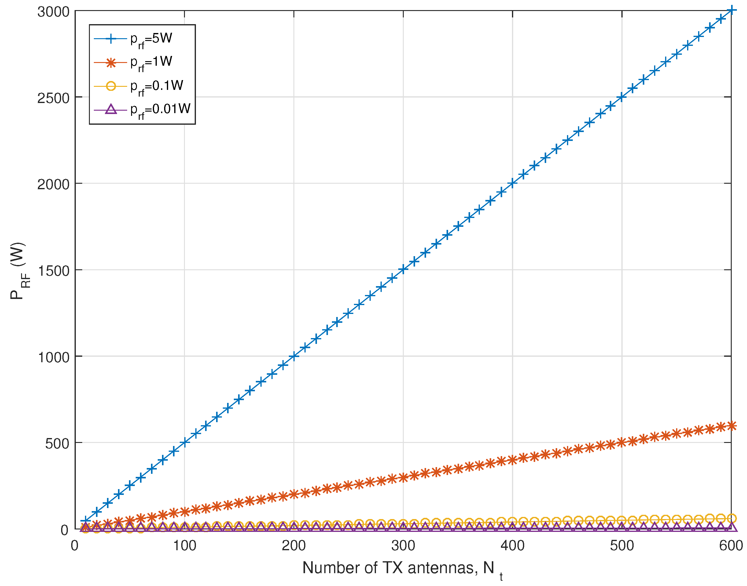
As mentioned beforehand, “RF components” refers to the DAC, mixer, and filter. Since an LSAS has an RF component for each antenna, the power consumption of RF components is significant. Figure 4 shows the RF power consumption versus the number of TX antennas, . In the case of W and , becomes 3000 W which is definitely not acceptable. There have been several studies aiming at overcoming this problem. It has been shown that since an LSAS can give significant channel gain, using coarse RF components with very low power consumption could be acceptable [8].
It is better to maintain the same level of RF power consumption regardless of TX antenna increase. Assuming low power RF components are well-designed, we chose W, when , similar to current BS systems.
There are several studies related to the RF component of LSAS [34,35,36]. In [34], a novel single-RF LSAS transmitter was presented. It comprises only a single power amplifier and does not require any mixer. It was shown that the total power efficiency of the transmitter in the LSAS regime is significantly higher than the total power efficiency in classical design. In [35], authors examined the effects of hardware impairments on a LSAS single-cell system. The simulations were performed using simplified, well-established statistical hardware impairment models as well as more sophisticated and realistic models based upon measurements and electromagnetic antenna array simulations. They demonstrated that low-resolution digital to analog converters decrease the overall power consumption while maintaining low average user received error vector magnitude and controlled unwanted emissions. The result showed that in LSAS, there is room for relaxing the stringent hardware requirements typically in place on current MIMO systems. In [36], authors analyzed the impact of RF hardware imperfections at the BSs by studying an uplink communication model with multiplicative phase-drifts, additive distortion noise, noise amplifications, and inter-carrier interference. According to their work, the key to cost-efficient deployment of large arrays is low-cost antenna branches with low circuit power, in contrast to today’s conventional expensive and power-hungry BS antenna branches. Such low-cost transceivers are prone to hardware imperfections, but they showed that the huge degrees-of-freedom would bring robustness to such imperfections.
4.3. Power Amplifier
The PA efficiency of current BS systems is around . Basically, the current BS systems use a digital pre-distorter and a peak-to-average power ratio reduction scheme to increase the efficiency of the power amplifier (PA). However, in LSASs, it is very difficult to use this kind of technique, because digital pre-distorter is an expensive device and must be applied to each antenna. Regarding the peak-to-average power ratio reduction scheme, the clipping scheme can be acceptable, since it is the most simple and effective peak-to-average power ratio reduction scheme. Due to this reason, we set the efficiency of the PA as for the LSAS. Figure 5 shows the PA efficiency versus peak-to-average powre ratio (dB) [21,22,37]. The PA efficiency is equivalent to 10 dB peak-to-average power ratio or Input Back-off. Since the peak-to-average power ratio of the OFDM signal, when B = 10 MHz with 1024 subcarriers, is around 11.7 dB with complementary cumulative distribution function, , we can say that around 1.7 dB is successfully reduced using any kind of scheme such as clipping.
There are several studies related to the PA of LSAS [38,39]. In [38], authors proposed a power amplifier configuration for LSAS transmitter. The proposed configuration consists of the amplifier path and the linear path which correspond to the signal cancellation loop of feed-forward configuration. The amplifier path comprises the vector regulator and the power amplifier, while the linear path comprises the delay line. Their results confirm the validity of the configuration employing the signal cancellation loop of 3.5-GHz 140-W class feed-forward power amplifier. In [39], authors proposed a more general EE model of LSAS considering PA efficiency as a variable, and investigated a power allocation algorithm based on zero-forcing precoding so that one can guarantee the TP and EE at the same time.
4.4. Precoding
For LSASs, as mentioned beforehand, there are two representative precoding schemes, ZF and MF precoding. Regarding power consumption, ZF consumes more than MF. However, the difference is small enough to not particularly affect overall power consumption. Figure 6 shows the difference in the power consumption of ZF and MF precoding using (14).
As observed, the power consumption difference between ZF and MF is only around 4 W even though we use 600 TX antennas. TP is one of the important factors that constitute EE. Figure 7 shows the TP difference between ZF and MF. For the simulations in this subsection, we assume perfect channel state information with no RS overhead to show the clear difference of ZF and MF. As can be seen, using ZF precoding gives (17.5 (bps/bps) → 29.4 (bps/bps)) improvement at compared to using MF precoding.
Based on Figure 6 and Figure 7, we present the EE difference between ZF and MF in Figure 8. ZF shows much better EE and the difference is more dominant as the number of TX antennas increases. When , ZF gives (85.5 ((bps/W)/(bps/W)) → 134 ((bps/W)/(bps/W))) better EE than MF. The analysis in this subsection supports the claim that ZF is much better than MF for both the TP and EE perspectives. However, in some applications, MF is much more useful than ZF. For example, in distributed TX antenna systems, to use ZF precoding, the distributed TX antenna systems need to know the channels of other distributed TX antennas. In this case, the backhaul burden could be too high to use ZF. MF does not requires the channel information of all distributed TX antennas. For this reason, MF is still a valuable option.
4.5. RS Overhead Reduction
The RS overhead of LSASs is a serious problem, because the RS overhead increases as increases. There are two kinds of channel estimation schemes, a scheme utilizing channel reciprocity (SUCR), and a scheme with no channel reciprocity (SNCR). The SUCR is a scheme where the BS estimates the channel for downlink precoding by using uplink signals. That is to say, the BS measures the downlink channel by using uplink signals. This means that when using SUCR, the number of RS for downlink channel measurements is proportional to the number of users, K. This kind of mechanism usually can be used for a time division duplex (TDD) system. Uplink/downlink channel calibration is necessary to use an uplink signal for downlink precoding. Using SNCR means the BS estimates the channel for precoding by using feedback signals from users. That is to say, the UE measures the channel by using the downlink RS. It indicates that the number of RS for downlink channel measurements is proportional to the number of TX antennas, . This kind of mechanism can be applicable for both TDD and frequency division duplex (FDD) systems.
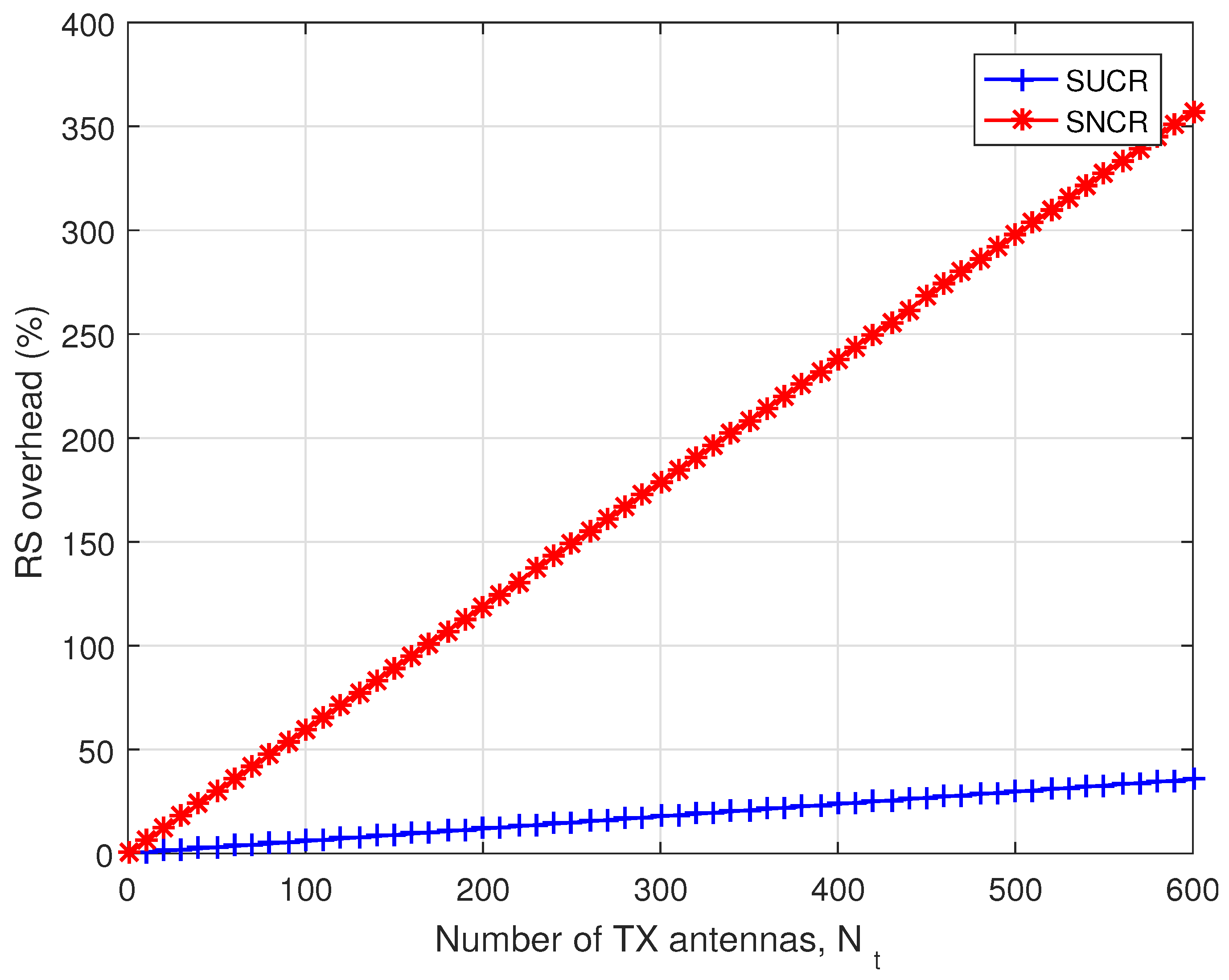
Figure 9 shows the RS overhead (%) versus the number of TX antennas, , for 1ms coherence time. In fact, SUCR does not use RS resources for downlink, however for fair comparison, we assume SUCR takes K RS and SNCR takes RS. If we increase , there is an opportunity to increase the co-scheduled K maintaining the minimum channel hardening effect of LSAS, . We also assume that the fundamental limit of RS overhead is , which corresponds to in the case of SNCR. If is more than 84, the RS takes more resources than the data signal, and it is not acceptable from the system performance point of view. If we use SUCR, even if we use , the RS overhead does not reach the limit, and thus we should use SUCR for the realization of LSAS. The fundamental problem of SUCR is the requirement of fine channel calibration. Because of uplink/downlink RF mismatch, uplink signals cannot be directly used for downlink precoding. A good calibration scheme is essential for the realization of SUCR based LSAS. Also, we assumed only one RS resource element is allocated to one user which is not enough for exact channel estimation in certain situations. Thus, we should keep in mind that RS overhead reduction accompanies channel estimation errors because the reduced RS causes an inaccurate estimation of channels.
4.6. Channel Estimation Error
As we witnessed in the previous subsection, the reduction of RS is inevitable in the realization of LSAS. As a result, due to insufficient RS, channel estimation errors are also inevitable. In this regard, we show TP variations with channel estimation errors in Figure 10 and Figure 11.
We modeled the estimated channel as follows,
where is the estimated channel matrix, is the error factor which reflects the degree of channel estimation error, and is the error matrix with the same statistical characteristic but independent of the channel. Using (24), the effective SINR of MF, and ZF precoding, can be represented as follows:
where is the channel estimation error vector.
where .
Then, TP and EE with channel estimation errors can be represented as:
where can be or depending on the situation. As we can see, the variation of TP and EE due to channel estimation errors is significant. For example, even when there is relatively high accuracy of the channel information, , in the case of ZF, the TP degradation is 43.18% (17.7 (bps/bps) → 10.0 (bps/bps)), and EE degradation is 43.36% (99.4 ((bps/W)/(bps/W)) → 56.3 ((bps/W)/(bps/W))). Table 3 shows the TP and EE when and .
Thus, preventing channel estimation errors is a key factor to increase EE. This will be discussed more in the next section.
5. Summary and Discussion
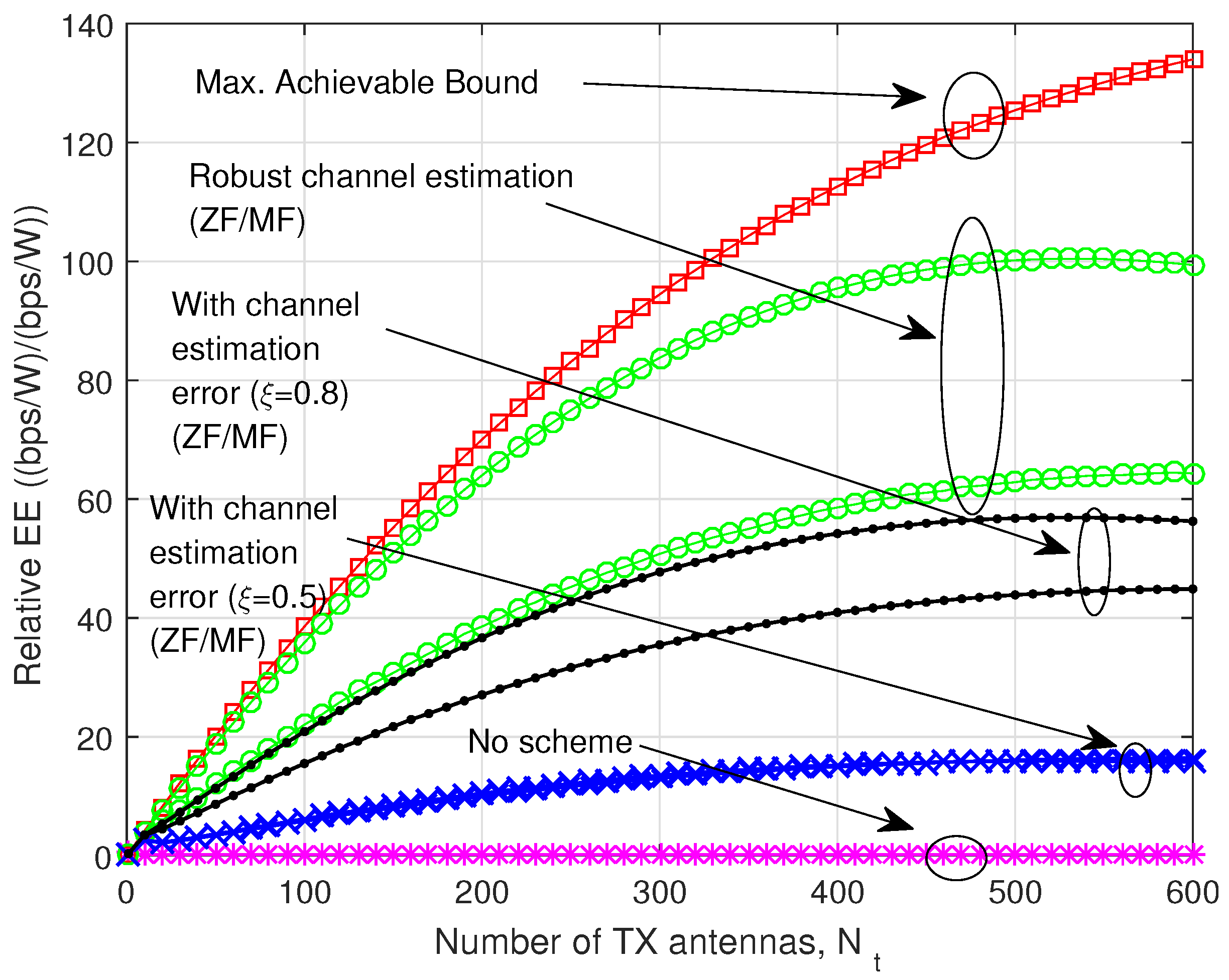
We summarize the expected throughput (TP) and EE gain of LSAS for each component with relevant schemes in Figure 12 and Figure 13. As observed, all of the mentioned technologies are important to increase EE. ‘No scheme’ indicates using existing BS technologies for the LSAS. As we can see, even though we can achieve a relative increase of TP as increases using existing technologies, there is no EE gain due to the high power consumption from RF components connected to each antenna. Once we achieve low power RF components with W and , there is a somewhat improvement in EE, however even though if the RS overhead reduction scheme is successfully applied, the TP/EE improvement is not so high. With RS overhead reduction and high precision channel estimation, we can achieve a relative TP of ((bps)/(bps)) and a relative EE of ((bps/W)/(bps/W)), when . This means with an TX antenna LSAS, we can reduce the carbon footprint around times compared to the current system. Maximum achievable bound indicates an ideal case with no RS overhead and perfect channel estimation. To achieve this, we need a perfect blind channel estimation scheme that is very difficult to achieve in real systems. Nevertheless, it can provide a very good reference for how much TP/EE gain can be achieved using an LSAS. As observed, once antenna and RF modules are appropriately implemented, the RS overhead and channel estimation errors are the dominant factors to overcome. The important point is that resolving only parts of issues can not increase the EE performance, that is, all the issues should be resolve together to enjoy the benefit of LSAS.
6. Conclusions
In this paper, we have presented the expected achievable gain of energy efficient cellular BSs with LSASs for Green ICT. Environmental pollution from ICT is on the rise, and it is very important to increase the EE of ICT to reduce the carbon footprint. In this regard, we have investigated the LSAS which can be used as a core signal transmission system, cellular BS that significantly increase the EE of ICT field. There are a lot of obstacles and necessary schemes for the realization of LSAS, and we have viewed related issues one by one and estimated how much EE gain can be achieved from each scheme. The cellular BS is one of the most power hungry ICT devices, thus increasing EE of the cellular BS is particularly important. We discussed the detailed research obstacles for the EE improvement of BS and showed that the obstacles should be solved together to improve the EE. We also showed that we can achieve 99.4 times EE improvement, and this figure can be a good reference for the future research. The main technical challenges of LSAS we pointed-out in the previous sections are (I) design of efficient antenna elements and antenna form factor; (II) design of low power PA/RF components; (III) channel estimation and reference signal overhead reduction. The compact antenna, and low power PA/RF components are related to implementation issues. Typically antenna form factor problem is diminished if we use high carrier frequency range, like mmWave range. However, we should overcome the poor channel condition. Low power PA/RF component is also an active research field. Due to the excessive channel gain, low power PA and relative coarse RF components could be also acceptable for LSAS. Channel estimation for LSAS is particularly difficult to resolve. Research related to using uplink channel sounding in time division duplexing (TDD) based system and using compressed feedback information are actively going-on. This paper can be a good reference for the realization of high EE BS, which gives a great benefit for environmental protection.
Acknowledgments
This work was supported by the National Research Foundation of Korea (NRF) grant funded by the Korea government (Ministry of Education) (NRF-2017R1D1A1B03028350), and faculty research fund of Sejong University in 2017.
Conflicts of Interest
The author declares no conflict of interest.
References
- Williams, E. Environmental Effects of Information and Communications Technologies. Nature 2011, 479, 354–358. [Google Scholar] [CrossRef] [PubMed]
- Despins, C.; Labeau, F.; Labelle, R.; Ngoc, T.L.; McNeil, J.; Leon-Garcia, A.; Cheriet, M.; Cherkaoui, O.; Lemieux, Y.; Lemay, M.; et al. Leveraging Green Communications for Carbon Emission Reductions: Techniques, Testbeds, and Emerging Carbon Footprint Standards. IEEE Commun. Mag. 2011, 49, 101–109. [Google Scholar] [CrossRef]
- Alsharif, M.H.; Kim, J. Optimal Solar Power System for Remote Telecommunication Base Stations: A Case Study Based on the Characteristics of South Korea’s Solar Radiation Exposure. Sustainability 2016, 8, 942. [Google Scholar] [CrossRef]
- Vereecken, W.; Van Heddeghem, W.; Colle, D.; Pickavet, M.; Demeester, P. Overall ICT footprint and green communication technologies. In Proceedings of the 4th International Symposium on Communications, Control and Signal Processing (ISCCSP), Limassol, Cyprus, 3–5 March 2010; pp. 1–6. [Google Scholar]
- Long, R.; Liu, J.; Lu, C.; Shi, J.; Zhang, J. Coordinated Optimal Operation Method of the Regional Energy Internet. Sustainability 2017, 9, 848. [Google Scholar] [CrossRef]
- Marzetta, T.L. Noncooperative Cellular Wireless with Unlimited Numbers of Base Station Antennas. IEEE Trans. Wirel. Commun. 2010, 9, 3590–3600. [Google Scholar] [CrossRef]
- Marzetta, T.L. Massive MIMO: An Introduction. Bell Labs Tech. J. 2015, 20, 11–22. [Google Scholar] [CrossRef]
- Björnson, E.; Larsson, E.G.; Marzetta, T.L. Massive MIMO: Ten myths and one critical question. IEEE Commun. Mag. 2016, 4, 114–123. [Google Scholar] [CrossRef]
- Tervo, O.; Le-Nam, T.; Markku, J. Optimal energy-efficient transmit beamforming for multi-user MISO downlink. IEEE Trans. Signal Process. 2015, 63, 5574–5588. [Google Scholar] [CrossRef]
- Tervo, O.; Tölli, A.P.; Juntti, M.; Tran, L.N. Energy-efficient coordinated beamforming with rate dependent processing power. In Proceedings of the IEEE 17th SPAWC, Edinburgh, UK, 3–6 July 2016. [Google Scholar]
- Xin, Y.; Wang, D.; Li, J.; Zhu, H.; Wang, J.; You, X. Area Spectral Efficiency and Area Energy Efficiency of Massive MIMO Cellular Systems. IEEE Trans. Veh. Technol. 2016, 65, 3243–3254. [Google Scholar] [CrossRef]
- Björnson, E.; Sanguinetti, L.; Hoydis, J.; Debbah, M. Designing multi-user MIMO for energy efficiency: When is massive MIMO the answer? In Proceedings of the IEEE WCNC 2014, Istanbul, Turkey, 6–9 April 2014; pp. 242–247. [Google Scholar]
- Ngo, H.Q.; Larsson, E.G.; Marzetta, T.L. Energy and Spectral Efficiency of Very Large Multiuser MIMO Systems. IEEE Trans. Commun. 2013, 61, 1436–1449. [Google Scholar]
- Wu, J.; Zhang, Y.; Zukerman, M.; Yung, E.K.N. Energy-efficient base-stations sleep-mode techniques in green cellular networks: A survey. IEEE Commun. Surv. Tutor. 2015, 17, 803–826. [Google Scholar] [CrossRef]
- Han, F.; Safar, Z.; Lin, W.S.; Chen, Y.; Liu, K.R. Energy-efficient cellular network operation via base station cooperation. In Proceedings of the IEEE International Conference on Communications (ICC), Ottawa, ON, Canada, 10–15 June 2012; pp. 4374–4378. [Google Scholar]
- Lee, B.M.; Kim, Y. Beam Grouping Based RS Resource Reuse and De-Contamination in Large Scale MIMO Systems. Appl. Sci. 2017, 7, 96. [Google Scholar] [CrossRef]
- Lee, B.M.; Kim, Y. Design of an Energy Efficient Future Base Station with Large-Scale Antenna System. Energies 2016, 9, 1083. [Google Scholar] [CrossRef]
- Spencer, Q.H.; Swindlehurst, A.L.; Haardt, M. Zero-Forcing Methods for Downlink Spatial Multiplexing in Multiuser MIMO Channels. IEEE Trans. Signal Process. 2004, 52, 461–471. [Google Scholar] [CrossRef]
- Peel, C.B.; Hochwald, B.M.; Swindlehurst, A.L. A Vector-Perturbation Technique for Near-Capacity Multiantenna Multiuser Communication—Part I: Channel Inversion and Regularization. IEEE Trans. Commun. 2005, 53, 195–202. [Google Scholar] [CrossRef]
- Lee, B.M.; de Figueiredo, R.J.P. Adaptive Predistorters for Linearization of High-Power Amplifiers in OFDM Wireless Communications. Circuits Syst. Signal Process. 2006, 25, 59–80. [Google Scholar] [CrossRef]
- Cripps, S.C. RF Power Amplifiers for Wireless Communications, 2nd ed.; Artech House: Norwood, MA, USA, 2006. [Google Scholar]
- Miller, S.L.; O’Dea, R.J. Peak Power and Bandwidth Efficient Linear Modulation. IEEE Trans. Commun. 1998, 46, 1639–1648. [Google Scholar] [CrossRef]
- Kumar, R.V.R.; Gurugubelli, J. How green the LTE technology can be? In Proceedings of the 2nd International Conference on Wireless Communication, Vehicular Technology, Information Theory and Aerospace & Electronic Systems Technology (Wireless VITAE), Chennai, India, 28 February–3 March 2011; pp. 1–5. [Google Scholar]
- Cui, S.; Goldsmith, A.J.; Bahai, A. Energy-Efficiency of MIMO and Cooperative MIMO Techniques in Sensor Networks. IEEE J. Sel. Areas Commun. 2004, 22, 1089–1098. [Google Scholar] [CrossRef]
- Marzetta, T.L. Preliminary Estimate of Computational Burden of LSAS: FLOPS and Watts; Green Touch: Cologny, Swiss, 2011. [Google Scholar]
- Yang, H.; Marzetta, T.L. Performance of Conjugate and Zero-Forcing Beamforming in Large-Scale Antenna Systems. IEEE J. Sel. Areas Commun. 2013, 31, 172–179. [Google Scholar] [CrossRef]
- Yang, H.; Marzetta, T.L. Total energy efficiency of cellular large scale antenna system multiple access mobile networks. In Proceedings of the IEEE Online Conference on Green Communications (GreenCom), Piscataway, NJ, USA, 29–31 Octorber 2013; pp. 27–32. [Google Scholar]
- Yang, H.; Marzetta, T.L. Energy efficient design of massive MIMO: How many antennas? In Proceedings of the 2015 IEEE 81st Vehicular Technology Conference (VTC Spring), Glasgow, UK, 11–14 May 2015; pp. 1–5. [Google Scholar]
- Dahlman, E.; Parkvall, S.; Skold, J. 4G: LTE/LTE-Advanced for Mobile Broadband; Academic Press: Cambridge, MA, USA, 2011. [Google Scholar]
- European Telecommunications Standards Institute (ETSI). ETSI Technical Report 136.931 Radio Frequency (RF) Requirements for LTE Pico Node B; Technical Report; ETSI: Sophia Antipolis, France, 2012. [Google Scholar]
- Wu, J. Green Wireless Communications: From Concept to Reality. IEEE Wirel. Commun. 2012, 19, 4–5. [Google Scholar] [CrossRef]
- Li, L.; Ali, M.; Haneda, K. Compact dual-band antenna array for massive MIMO. In Proceedings of the 2016 IEEE 27th PIMRC, Valencia, Spain, 4–8 September 2016. [Google Scholar]
- Manteuffel, D. Compact multi port multi element antenna for Massive MIMO. In Proceedings of the 2016 IEEE APSURSI, Fajardo, Puerto Rico, 26 June–1 July 2016. [Google Scholar]
- Sedaghat, M.A.; Mueller, R.R.; Mueller, R.R.; Fischer, G. A Novel Single-RF Transmitter for Massive MIMO. In Proceedings of the 18th WSA 2014, Erlangen, Germany, 12–13 March 2014. [Google Scholar]
- Gustavsson, U.; Sanchéz-Perez, C.; Eriksson, T.; Athley, F.; Durisi, G.; Landin, P.; Hausmair, K.; Fager, C.; Svensson, L. On the impact of hardware impairments on massive MIMO. In Proceedings of the 2014 IEEE Globecom, Austin, TX, USA, 8–12 December 2014. [Google Scholar]
- Björnson, E.; Matthaiou, M.; Debbah, M. Massive MIMO with Non-Ideal Arbitrary Arrays: Hardware Scaling Laws and Circuit-Aware Design. IEEE Trans. Wirel. Commun. 2015, 14, 4353–4368. [Google Scholar] [CrossRef]
- Wulich, D. Definition of Efficient PAPR in OFDM. IEEE Commun. Lett. 2005, 9, 832–834. [Google Scholar] [CrossRef]
- Suzuki, Y.; Narahashi, S. Power Amplifier Configuration for Massive-MIMO Transmitter. In Proceedings of the 22th APCC 2016, Yogyakarta, Indonesia, 25–27 August 2016. [Google Scholar]
- Guo, Y.; Tang, J.; Wu, G.; Li, S. Power allocation for massive MIMO: Impact of power amplifier efficiency. In Proceedings of the IEEE ICCC, Shenzhen, China, 2–4 November 2015. [Google Scholar]
Figure 1.
Shannon’s channel capacity versus .
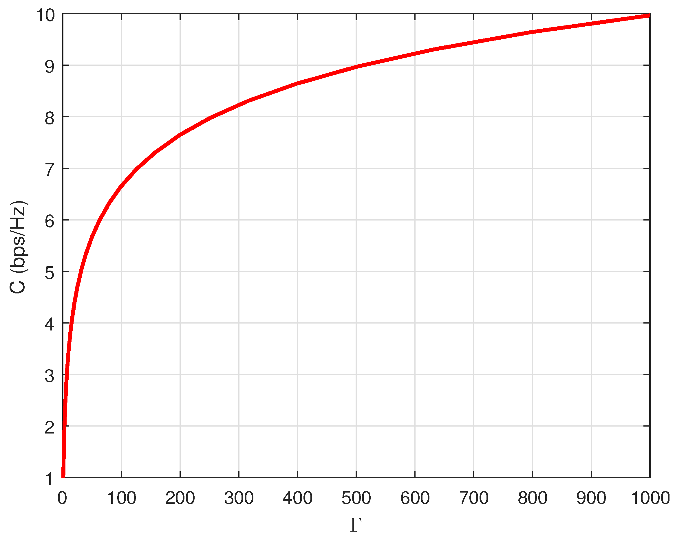
Figure 2.
Change of Performance metric from TP to EE.
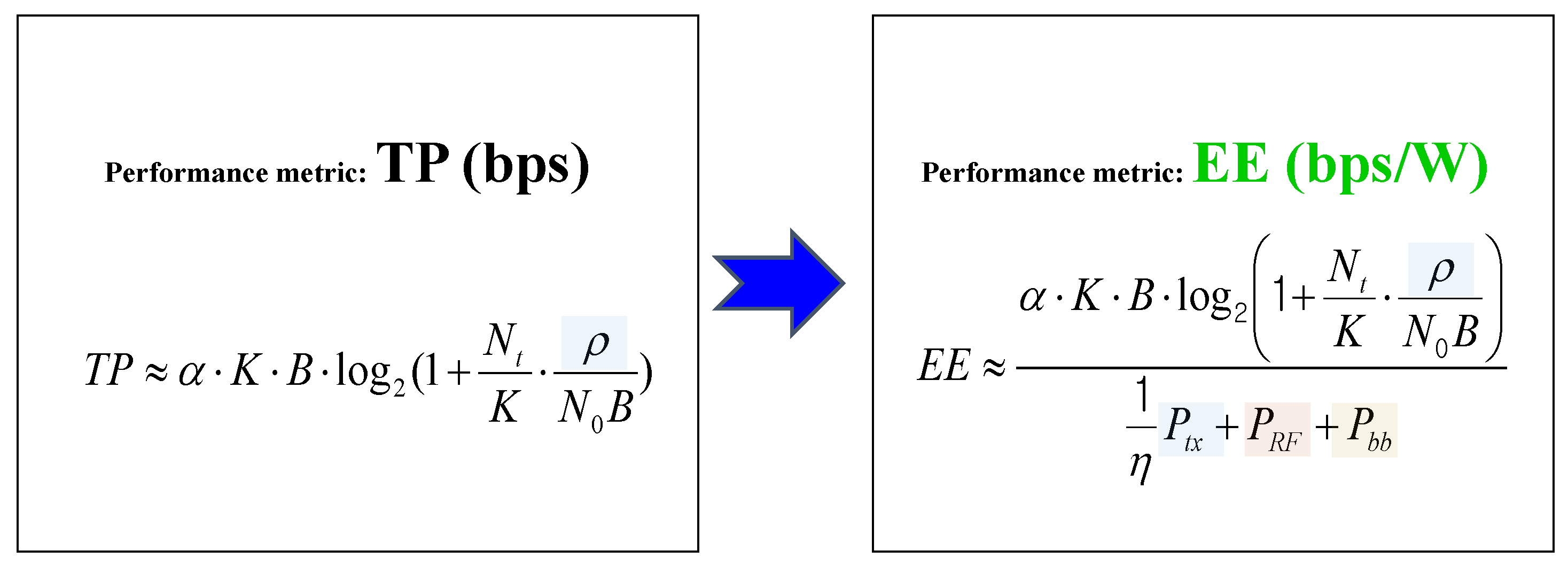
Figure 3.
Examples of antenna form factor with 400 (20 × 20) antennas, antenna spacing ∼, and carrier frequencies of 2 GHz and 6 GHz.
Figure 3.
Examples of antenna form factor with 400 (20 × 20) antennas, antenna spacing ∼, and carrier frequencies of 2 GHz and 6 GHz.
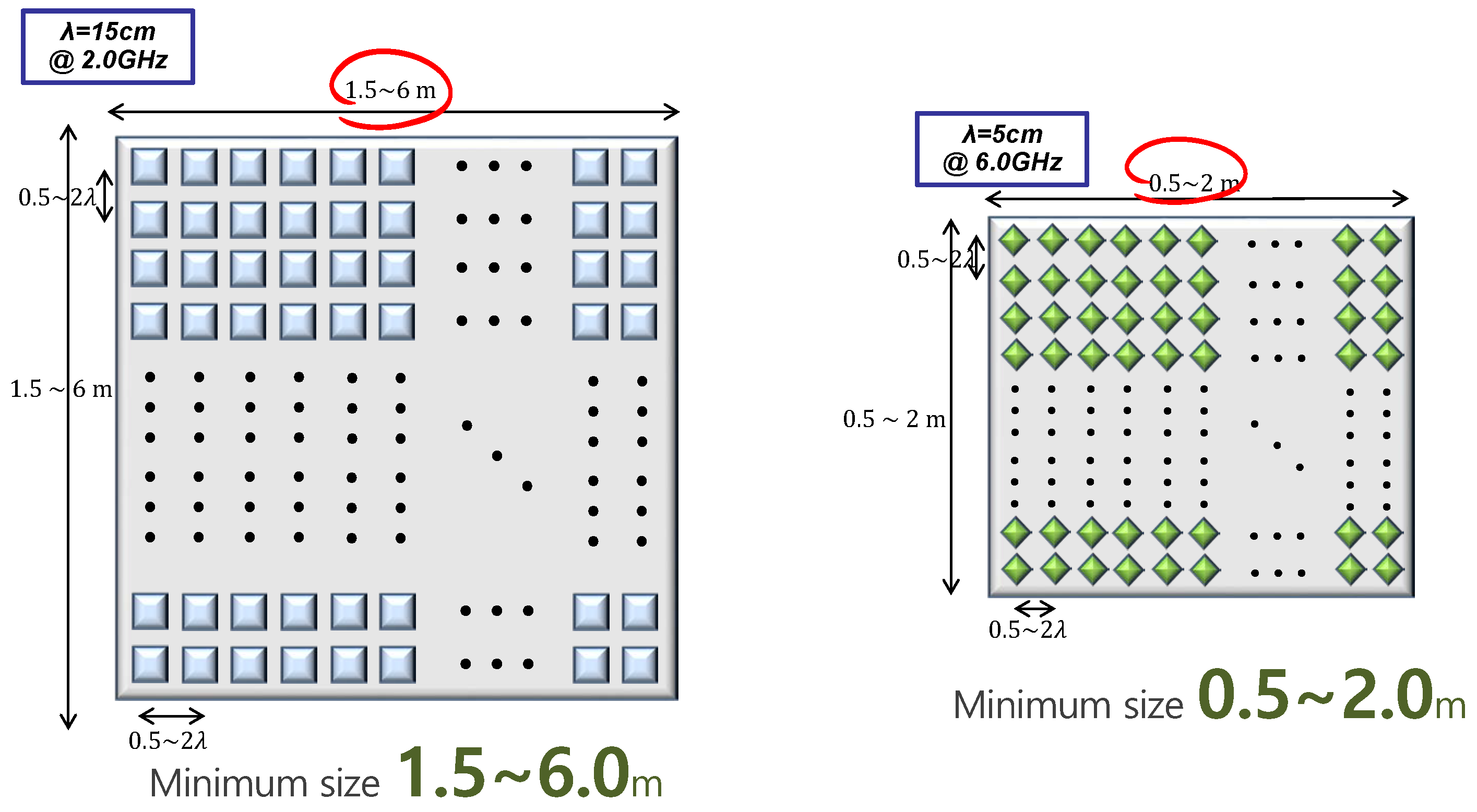
Figure 4.
as increases.

Figure 5.
PA efficiency, versus peak-to-average power ratio (PAPR) (dB).
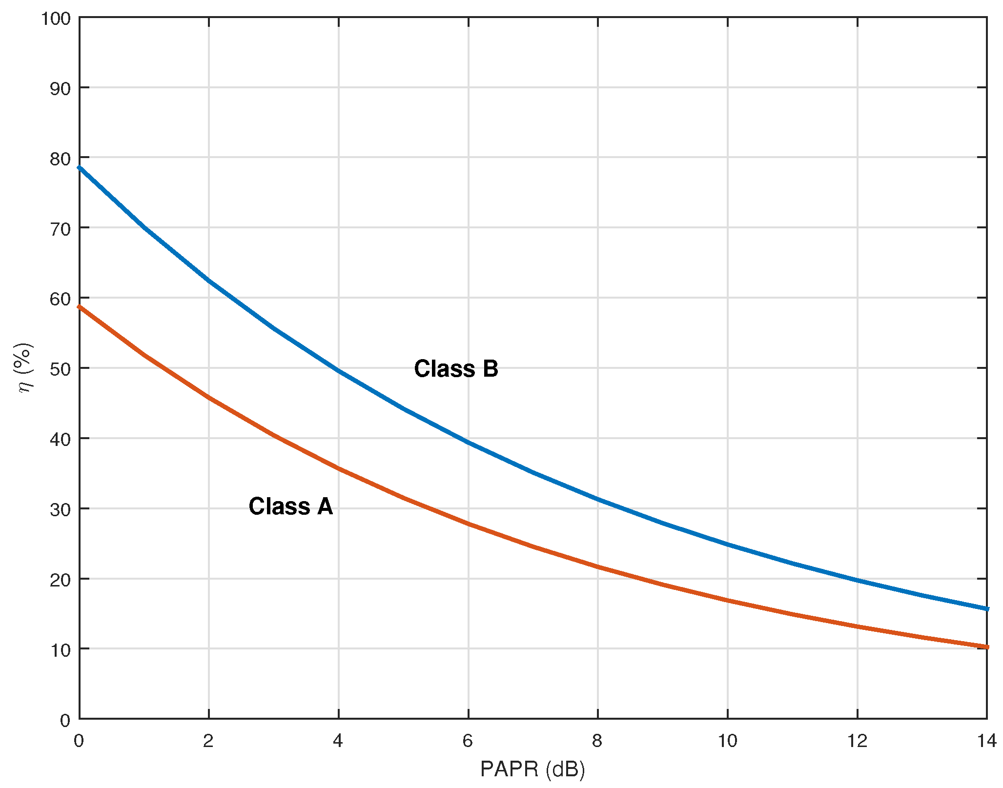
Figure 6.
as increasing , when using ZF and MF precoding with .
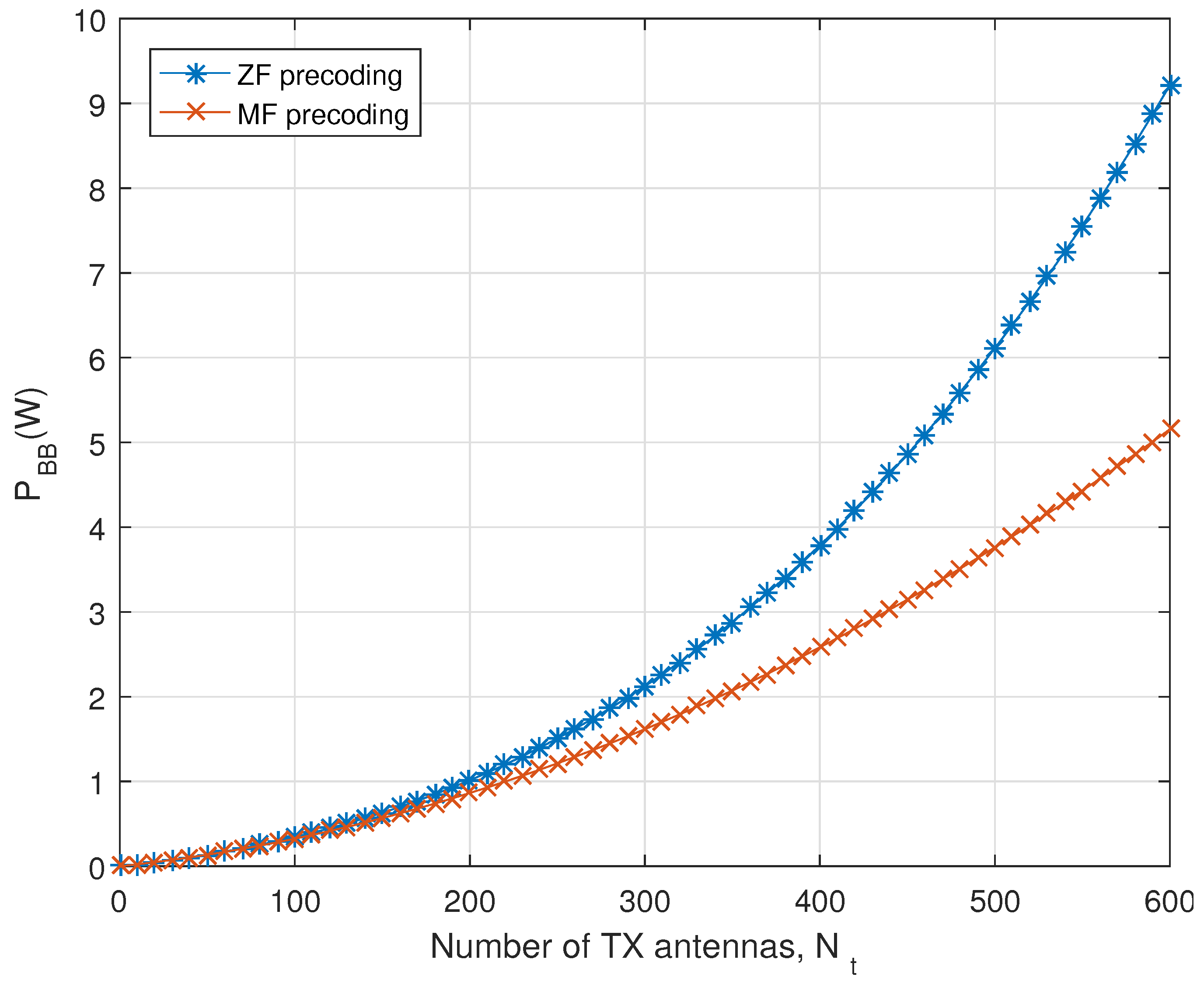
Figure 7.
TP difference between ZF and MF.

Figure 8.
EE difference between ZF and MF.
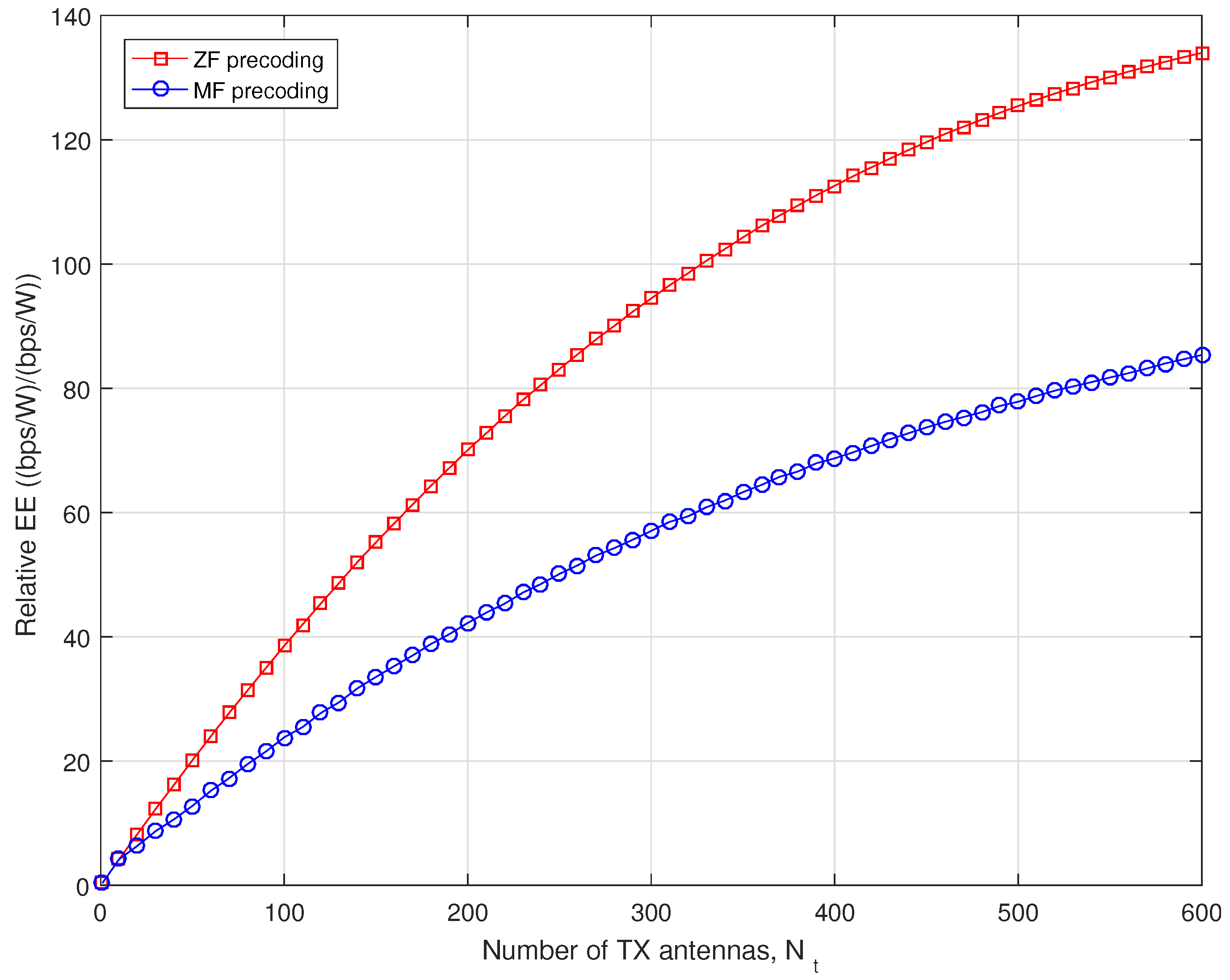
Figure 9.
RS overhead (%) versus the number of TX antennas, for 1ms coherence time.

Figure 10.
TP variations with channel estimation errors, (a) ZF precoding; (b) MF precoding.
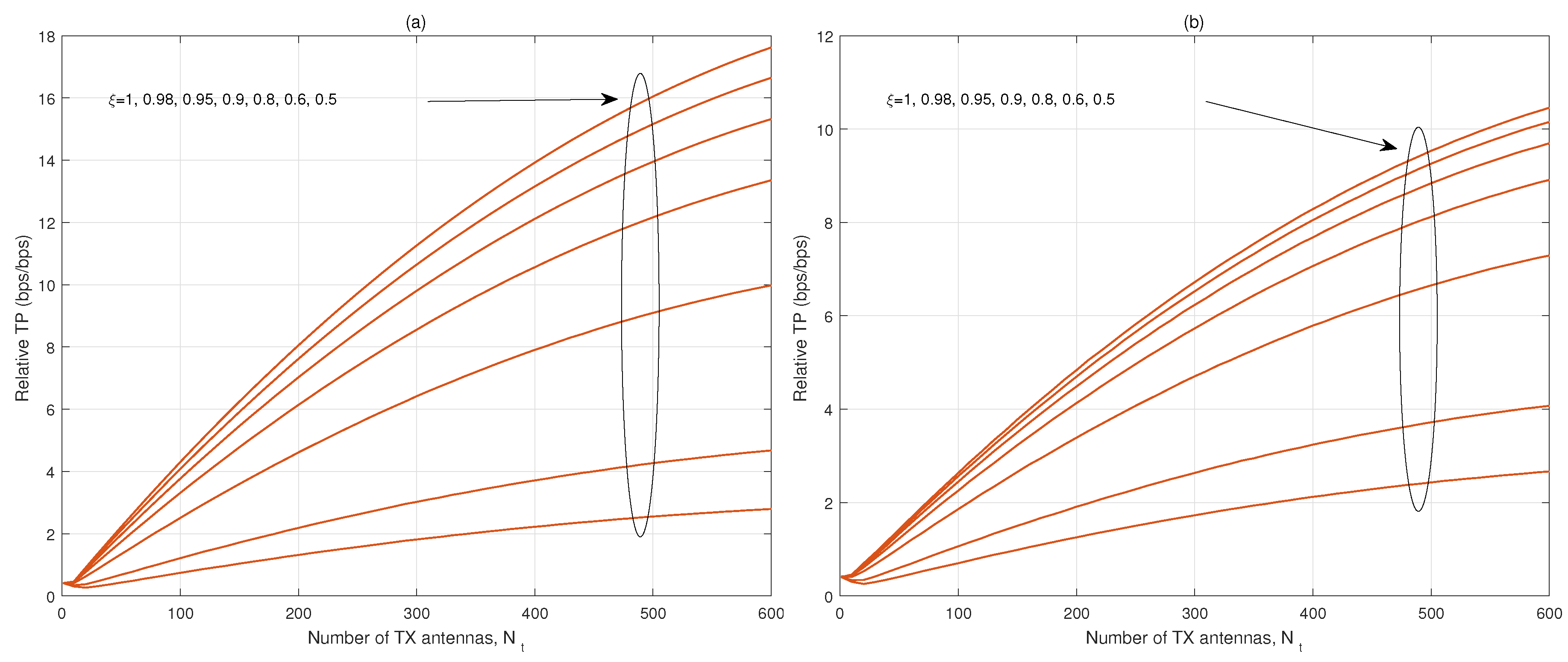
Figure 11.
EE variations with channel estimation errors, (a) ZF precoding, (b) MF precoding.
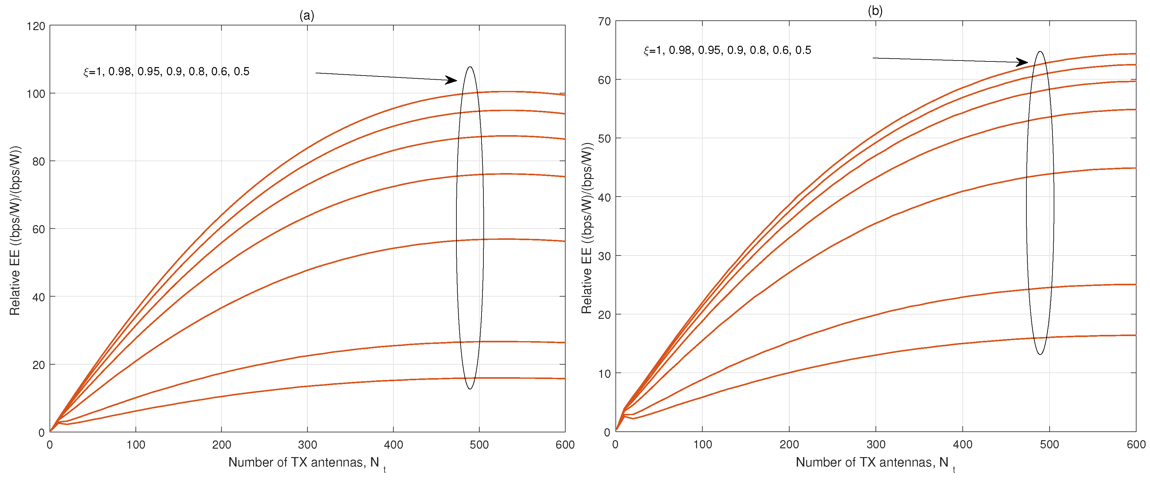
Figure 12.
Relative TP gain as increases.
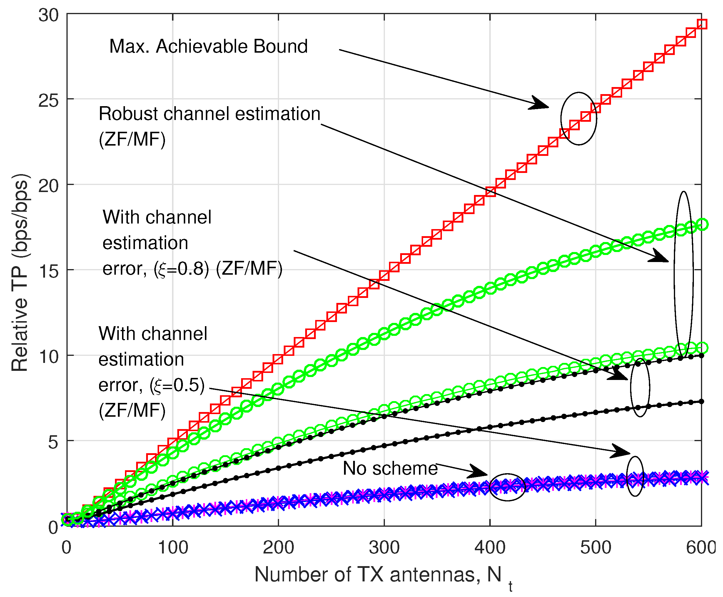
Figure 13.
Relative EE gain as increases.

Table 1.
Precoding matrices of MF, ZF, and RZF.
| MF | ZF | RZF | |
|---|---|---|---|
Table 2.
System Parameters.
| Parameter | Description | Value |
|---|---|---|
| B | Bandwidth | 10 MHz |
| Slot length | ms | |
| Pilot length in one slot | ms | |
| Symbol duration | us | |
| Guard Interval (GI) | us | |
| Symbol without GI | us | |
| Delay spread | us |
Table 3.
Relative TP (bps/bps) and EE ((bps/W)/(bps/W)).
| TP | EE | |||
|---|---|---|---|---|
| ZF | MF | ZF | MF | |
| 1 | 17.6 | 10.5 | 99.4 | 64.4 |
| 0.8 | 10.0 | 7.3 | 56.3 | 44.9 |
© 2017 by the author. Licensee MDPI, Basel, Switzerland. This article is an open access article distributed under the terms and conditions of the Creative Commons Attribution (CC BY) license (http://creativecommons.org/licenses/by/4.0/).
Share and Cite
MDPI and ACS Style
Lee, B.M. Energy Efficiency Gain of Cellular Base Stations with Large-Scale Antenna Systems for Green Information and Communication Technology. Sustainability 2017, 9, 1123. https://doi.org/10.3390/su9071123
AMA Style
Lee BM. Energy Efficiency Gain of Cellular Base Stations with Large-Scale Antenna Systems for Green Information and Communication Technology. Sustainability. 2017; 9(7):1123. https://doi.org/10.3390/su9071123
Chicago/Turabian StyleLee, Byung Moo. 2017. "Energy Efficiency Gain of Cellular Base Stations with Large-Scale Antenna Systems for Green Information and Communication Technology" Sustainability 9, no. 7: 1123. https://doi.org/10.3390/su9071123
Note that from the first issue of 2016, this journal uses article numbers instead of page numbers. See further details here.