Making Marine Noise Pollution Impacts Heard: The Case of Cetaceans in the North Sea within Life Cycle Impact Assessment

Industrial Ecology Programme, Department for Energy and Process Engineering, Norwegian University of Science and Technology (NTNU), 7491 Trondheim, Norway
*
Author to whom correspondence should be addressed.
Sustainability 2017, 9(7), 1138; https://doi.org/10.3390/su9071138
Submission received: 6 April 2017
/
Revised: 18 June 2017
/
Accepted: 26 June 2017
/
Published: 28 June 2017
(This article belongs to the Section Sustainable Engineering and Science)
Abstract
:Oceans represent more than 95% of the world’s biosphere and are among the richest sources of biodiversity on Earth. However, human activities such as shipping and construction of marine infrastructure pose a threat to the quality of marine ecosystems. Due to the dependence of most marine animals on sound for their communication, foraging, protection, and ultimately their survival, the effects of noise pollution from human activities are of growing concern. Life cycle assessment (LCA) can play a role in the understanding of how potential environmental impacts are related to industrial processes. However, noise pollution impacts on marine ecosystems have not yet been taken into account. This paper presents a first approach for the integration of noise impacts on marine ecosystems into the LCA framework by developing characterization factors (CF) for the North Sea. Noise pollution triggers a large variety of impact pathways, but as a starting point and proof-of-concept we assessed impacts on the avoidance behaviour of cetaceans due to pile-driving during the construction of offshore windfarms in the North Sea. Our approach regards the impact of avoidance behaviour as a temporary loss of habitat, and assumes a temporary loss of all individuals within that habitat from the total regional population. This was verified with an existing model that assessed the population-level effect of noise pollution on harbour porpoises (Phocoena phocoena) in the North Sea. We expanded our CF to also include other cetacean species and tested it in a case study of the construction of an offshore windfarm (Prinses Amalia wind park). The total impact of noise pollution was in the same order of magnitude as impacts on other ecosystems from freshwater eutrophication, freshwater ecotoxicity, terrestrial acidification, and terrestrial ecotoxicity. Although there are still many improvements to be made to this approach, it provides a basis for the implementation of noise pollution impacts in an LCA framework, and has the potential to be expanded to other world regions and impact pathways.
1. Introduction
The world’s oceans are important for all life on Earth, including human well-being [1]. Global economies and communities are dependent on the natural assets and the services that oceans provide. Nearly three billion people rely on fish as their main source of protein [2], and more than 10% of the global human population depends on the fishery and aquaculture industry for their livelihood [3]. Oceans are also increasingly important for recreation and tourism, and crucial for international shipping transport [4]. Indirectly, oceans benefit human well-being by producing nearly 50% of the oxygen and absorbing one-third of the CO2 in our atmosphere [5]. The total economic benefits generated by ocean sources are estimated to be worth at least 2.5 trillion U.S. dollars each year [6].
Nevertheless, humanity is mismanaging the oceans [4]. The average per capita consumption of fish is increasing rapidly [2], because of both capture fisheries and aquaculture. Aquaculture operations may lead to noise impacts on both captive species and wild species in the surrounding [7,8]. Simultaneously, ship traffic (including for capture fisheries) today is three times larger than it was two decades ago [9], and more than one-third of oil and gas comes from offshore sources [10]. All these industrial activities are expected to expand even further due to the growth of human population [2], exacerbating pressures such as overexploitation, pollution, and destruction of habitats [4]. At the same time, only 3.4% of marine ecosystems are under protection, of which only parts are effectively managed [4]. The Living Blue Planet Report 2015 by the World Wide Fund for Nature (WWF) presented alarming declines in marine biodiversity, estimating that average population levels of marine vertebrate species have a
lmost halved over the last forty years [4]. These trends may have impacts throughout the whole food web and ultimately change marine ecosystem functioning in general [11].
One pressure that is expected to increase and is considered to be an emerging issue of great detriment to ecosystems is noise pollution [12,13]. In water, sound propagation is greater than light, and therefore marine life has evolved to use sound for communication, feeding, navigation, and for their perception of the environment around them [14,15]. Sound is thus of critical importance to the survival of marine animal species, particularly for fish and mammals [14,16]. Noise pollution can therefore contribute to substantial stress and loss of biodiversity [17]. Multiple studies report evidence of death of individuals, reductions in population numbers, decreases in species diversity, damage to hearing organs, increases in stress levels and disruptive behaviour, as well as habitat displacement [11,18,19,20,21,22,23]. Noise pollution is considered a serious threat [12,14]. However, the fact that underwater noise pollution is of concern for marine biodiversity has only recently reached recognition on both a scientific and managerial level. The International Whaling Commission (IWC) discusses the issue of noise impacts on whales (e.g., from pile driving) as well and gives recommendations regarding the problems of underwater noise in several reports (e.g., [24,25]). However, the impacts are still not covered in any decision-support tools. To effectively implement regulations on underwater noise pollution, and therefore mitigate its impacts, a good understanding of how potential environmental impacts are related to industrial processes is required and needs to be implemented in decision-support tools. A method that can be used for this purpose is life cycle assessment (LCA). LCA systematically assesses the environmental impacts of a product or service over its entire life cycle, from which opportunities for improvement can be identified [26,27]. In the life cycle impact assessment (LCIA) phase, the environmental significance of the emissions and used resources collected in the life cycle inventory is evaluated [27] with the help of characterization factors (CF) (see also Figure 1). LCIA quantifies the contribution of each emission or used resource to different environmental impacts, per unit of product or service; the functional unit (FU) [28], such as the environmental impact of transporting a product over a certain distance. Models characterize impacts via midpoint indicators (indicating the potential impact at a chosen location along the impact pathway), and continue towards endpoint level indicators (indicating potential ecosystem damage) [29]. Normally, endpoint indicators are aggregated into three areas of protection (AoP): human health, ecosystem quality, and resource scarcity [30]. For our purposes of method development, only ecosystem quality is relevant.
Although some effort to include the impacts of noise on human health exist [31,32,33], there is currently no globally operational characterization factor (CF) for noise pollution impacts on human health in general and no approach exists for impacts on ecosystems. The aim of this paper is to present first steps towards an operational approach for integrating noise pollution impacts on marine ecosystems into the LCA framework, by developing preliminary CFs for noise impacts on cetaceans in the North Sea from pile driving. We test the relevance and applicability of this CF in a case study of offshore wind power production (see choice of impact pathway in Section 2.1). We are aware of the limitations of our study in terms of geographical and taxonomic coverage, as well as data input and complexity for more fine-scaled models. We, therefore, conclude this paper by making recommendations for urgently needed research.
2. Material and Methods
2.1. Choice of Impact Pathway and Affected Species
The marine environment contains many different species, both plants and animals, but the effects of underwater noise pollution have only been studied on animal species so far. As shortly described earlier and shown in different articles (e.g., [34,35,36,37], the effects of marine noise on marine species are manifold, depending on the noise source and species’ sensitivity. Anthropogenic ocean noise can come from many different sources, such as marine traffic, seismic exploration, sonar, deterrent devices, and construction work [38]. Depending on the sound intensity, the effects range from physical injuries and hearing loss, to masking of communication, behavioural changes, and increased stress levels [39]. The large range of noise sources and different effects results in a large variety of pathways in which the marine environment can be impacted by noise pollution. However, for simplicity, we will focus on one pathway to start with, i.e., one effect from one noise source on one species.
From the amount of literature on noise pollution impacts available, it can be concluded that marine mammals, and in particular cetaceans, are the most sensitive species (e.g., [40,41]). In addition, they are regarded as the best bioindicator of the ocean’s acoustic tolerance limit, because of their exclusive dependence on acoustics for their survival [41]. Cetaceans were therefore chosen as the species group of interest for this study.
The choice of noise source and its effect was based on a trade-off analysis between available studies, based on the quality and the quantity of their available data required in an LCA context, the modelling potential of the impact pathway for inclusion in an LCA framework, and the increasing importance of the noise source. A total of 23 studies containing quantitative data were assessed by assigning qualitative weights on a scale from zero to five to the different parts (data availability, modelling potential, etc.). A list with all studies and weights can be found in the Supplementary Materials (Excel file). We are aware that there are many more ecological studies describing effects of different noise sources on cetaceans and do not aim to perform a comprehensive analysis here. The highest score was found for a study that presents the impacts of pile-driving activities during the construction of offshore wind farms on the harbour porpoise in terms of avoidance behaviour [42]. This study was thus taken as a starting point. This study builds on a model that assesses the population consequences of disturbance (PCoD) of marine mammals [43] in order to assess the cumulative effects of impulsive underwater sound from the pile-driving activities during the construction of offshore wind farms on the harbour porpoise population in the North Sea [42]. The relevance of the chosen impact pathway and species is highlighted by a substantial amount of ecological literature related to the impacts of pile driving on harbour porpoises (see e.g., [44,45,46,47,48]). The PcOD model is also described in more detail in New et al. [49]. The model is based on case studies of different species (e.g., elephant seals and beaked whales) and is a further development of the PCAD model, in order to include other disturbances than just noise and to include effects both on the behaviour and the physiology of the species [50]. The PCAD model (Population Consequences of Acoustic Disturbance) was originally developed by the National Research Council of the United States [51].
2.2. Constructing the Characterization Factor
To construct a characterization factor (CF) for the avoidance behaviour of harbour porpoises due to pile-driving during the construction of offshore wind farms, the approach by Heinis et al. [42] was combined with the multi-step framework from Cucurachi et al. [31], as explained further below. In general, models for developing CFs for impacts on ecosystems in LCA consist of two to three parts: (1) a fate factor (telling us how an emission distributes in the environment); (2) an exposure factor (quantifying how many species/taxonomic groups are exposed and how the emission reaches them); and (3) an effect factor (describing the consequences of the emission on the species, e.g., death or reduced functionality) [30]. Often, exposure and effect factor are combined as one factor (also called effect factor).
2.2.1. Sound Propagation and Fate Factor
To determine the environmental significance of a sound emission, the amount of sound that reaches the receiver has to be known. The approach for determining this used by Cucurachi et al. [31] is slightly different from the approach used by Heinis et al. [42]. Cucurachi et al. [31] define a fate factor as a marginal increase of the sound pressure received, due to a marginal increase of the sound power emitted, compared to the ambient background level. Since for most areas the ambient background level is unknown in marine ecosystems, this is not a convenient approach. What the two approaches agree on is that the fate factor for noise pollution refers to the propagation of sound, and thus how much of the emitted sound reaches the receiver. Heinis et al. [42] use the sound exposure level (SEL) as a measure for the sound level that is received by an animal. This is defined as the “decibel level of the cumulative sum-of-square pressures over the duration of a sound for sustained nonpulse sounds where the exposure is of a constant nature” [16]. The approach from Heinis et al. [42] calculates a single exposure equivalent of the constant sound, and assumes that no recovery of the animal takes place between exposures. The sound level at the source and the propagation loss in the environment have to be known to calculate the SEL received by an animal. The sound level that is received by an animal equals the emitted sound level by the source minus the propagation loss PL due to environmental conditions such as salinity, temperature, and bathymetry.
Heinis et al. [42] use the sound propagation model AQUARIUS, developed by the Netherlands Organisation for Applied Scientific Research (TNO), to calculate the loss of sound and subsequently the SELs around a sound source. They also produce sound maps to visualize the sound levels in an area. The AQUARIUS model, however, was unavailable to us. Other open-source sound propagation models are available, but require not only the sound level from the source as an input but also data on the bathymetry of the area, wind speed, or other environmental conditions. This data is often unavailable (or has high uncertainties). Therefore, we used a simplified method to calculate sound propagation based on only spherical spreading loss, described by Equation (1) [52].
where PL is the propagation loss in dB and R is the distance from the sound source in metres.
This is a simplification of reality due to a lack of data, but has been used before for modelling acoustic propagation in marine environments [53]. Source levels are generally calculated by back-propagating measured SELs using only spherical spreading loss [52], as is the case in the study by Heinis et al. [42]. They assumed that for the calculation of the propagation of piling noise, the measurements from the Prinses Amalia wind park (PAWP) (a wind park off the coast of The Netherlands), as presented by de Jong and Ainslie [54], can be used as a basis for all noise estimations of monopile driving in the North Sea. De Jong and Ainslie [54] included noise measurements from other pile-driving activities at several distances between 1 km and 10 km, and found that the trend of spherical spreading loss provided a good fit. They measured that at a distance of 1 km, the SEL of the PAWP was 172 dB re 1 µPa2-s. Because we know that the received SEL at 1 km equals the emitted sound level minus the propagation loss at 1 km, the value of 172 dB re 1 µPa2-s can be back-propagated to obtain the emitted sound level. We then used this emitted sound level to calculate the SELs over a larger range of distances.
2.2.2. Affected Animals and Modelling of a Midpoint Characterization Factor
For calculating a midpoint characterization factor, the sound propagation (fate factor) is combined with an exposure factor, which is describing the exposure to the noise impact on a population due to an emission, in numbers of affected animals. In toxicity, it is common to use a critical level of an emission from a dose–response curve [55]. However, for noise pollution such curves only exist for one impact pathway: the probability of harassment from sonar on odontocetes and mysticetes [56]. Because neither the data nor a dose–response curve exist for our impact pathway of interest, we follow the approach of Heinis et al. [42] of using a threshold level of 136 dB for avoidance behaviour of harbour porpoises, which was derived from a study on behavioural responses of harbour porpoises to different sound levels [42]. Any behaviour with a response score of 5 or higher on the severity scale presented by [16] was considered avoidance behaviour [42]. It should be noted that the methodology by Southall et al. has been criticized for not being applicable to countries other than the U.S. because it is targeted towards its policies [48] and also because it is based on a few captive animals, which may insufficiently reflect the response of wild animals [57]. Nevertheless, we think it is still a sufficiently good approach for a first attempt at integrating noise impacts into an LCIA framework.
Combining the sound propagation calculation from Equation (1) with the threshold level for avoidance, the avoidance distance and subsequently the avoidance area (assumed to be circular) can be calculated (see Equation (2)). Offshore wind farms are often constructed close to the shore, and thus part of the circle that the avoidance distance forms will be on land and will not affect the marine ecosystem. The PAWP was constructed at a distance of 26 km from the Dutch coast. By standard calculations for a circular area segment, and the assumption of a straight shoreline, the area of the part of the circle that covers land can be calculated and subtracted from the circular area to obtain the final avoidance area [58].
For the effect factor for human health, Cucurachi et al. [31] looked at three aspects that are relevant: (1) the frequency-dependency of the perception of humans; (2) the time of day of the exposure; and (3) the number of humans in the exposed area. All of these can be adapted to fit marine species, as explained below.
Southall et al. [16] present a method to calculate the frequency-weighting of a sound to different marine mammal functional hearing groups. This weighting can be applied to the sound level that an animal receives. We applied it to calculate the threshold levels for other species than the harbour porpoise, and will elaborate on this in Section 2.4.1.
The time of day of the exposure is of less importance to marine species. Instead, we take seasonal variability into account, by using the number of harbour porpoises in the exposed area during different seasons [42,59], thus combining aspects two and three of Cucurachi et al. [31]. The distribution of the harbour porpoise in the North Sea is described in Geelhoed et al. [59] and shows that the animal density differs over four regions of the North Sea and between seasons (surveys for spring, summer, and late autumn/winter).
Heinis et al. [42] then calculate the number of “harbour porpoise disturbance days” by multiplying the avoidance area by the population density and the total number of disturbance days (the days on which sound impulses take place) of the project. For an LCA framework, we regard the impact of avoidance behaviour as a temporary loss of habitat, and assume a temporary loss of all individuals within that habitat. A disturbance day is assumed to last 24 h, disregarding the actual duration of the noise from pile-driving during that day. During this disturbance day, all individuals within the avoidance area are assumed to be lost (displaced). After the disturbance day, the situation is assumed to be back to normal, i.e., the animals return to the area immediately. Thus, the midpoint CF is calculated by multiplying the avoidance area (in km2) by the population density (in animals per km2) and the fraction of the year that the disturbance takes place, summing over season s, as shown in Equation (2) below. In order to facilitate application in LCA studies, we provide the CF on a yearly instead of a seasonal basis. The unit of the midpoint CF is comparable to the number of people that are exposed to noise by Cucurachi et al. [31].
This characterization factor can be calculated either on a regional or local scale using data from Geelhoed et al. [59]. Regional in this case means for the whole North Sea ecosystem, and local corresponds to only one out of the four regions defined by Geelhoed et al. [59]. For many other marine species, however, these local distribution numbers may not be available. In that case, using population densities for the whole ecosystem in general, only a regional impact (i.e., on ecosystem level) can be calculated. This study does not look at impacts on a global scale.
2.2.3. Endpoint Modelling
To calculate the impact of the number of affected harbour porpoises on a population level, we divide the affected individuals per year by the total population of harbour porpoises in the North Sea, resulting in a potentially disappeared fraction of species (PDF) (the species disappear temporarily from the area). By multiplying this fraction by the total number of years that the disturbance will take place, and dividing by the total production of electricity [kWh] over a lifetime of the wind park, we obtain a characterization factor on the endpoint level (PDFpop·yr/kWh) (Equation (3)). PDF is a commonly used unit for the area of protection ecosystem quality [60,61,62]. We are thus in line with this tradition, even though our indicator indicates the disappearance within one population (therefore subscript “pop”, for population is added) and not across species diversity, as usual. Thus, essentially, the midpoint CF (Equation (2)) is divided by the total number of individuals found in the ecosystem, in this case the North Sea (, and the total production in kWh over the lifetime of the wind park (
In addition, is the avoidance area corresponding to the specific species (km2), is the number of disturbance days per year, and is the population density i.e., the number of individuals per square kilometre (either locally or regionally). The division by the total population number transforms the absolute loss of individuals into a fraction of species that are lost from this population.
2.3. Verification of the Method
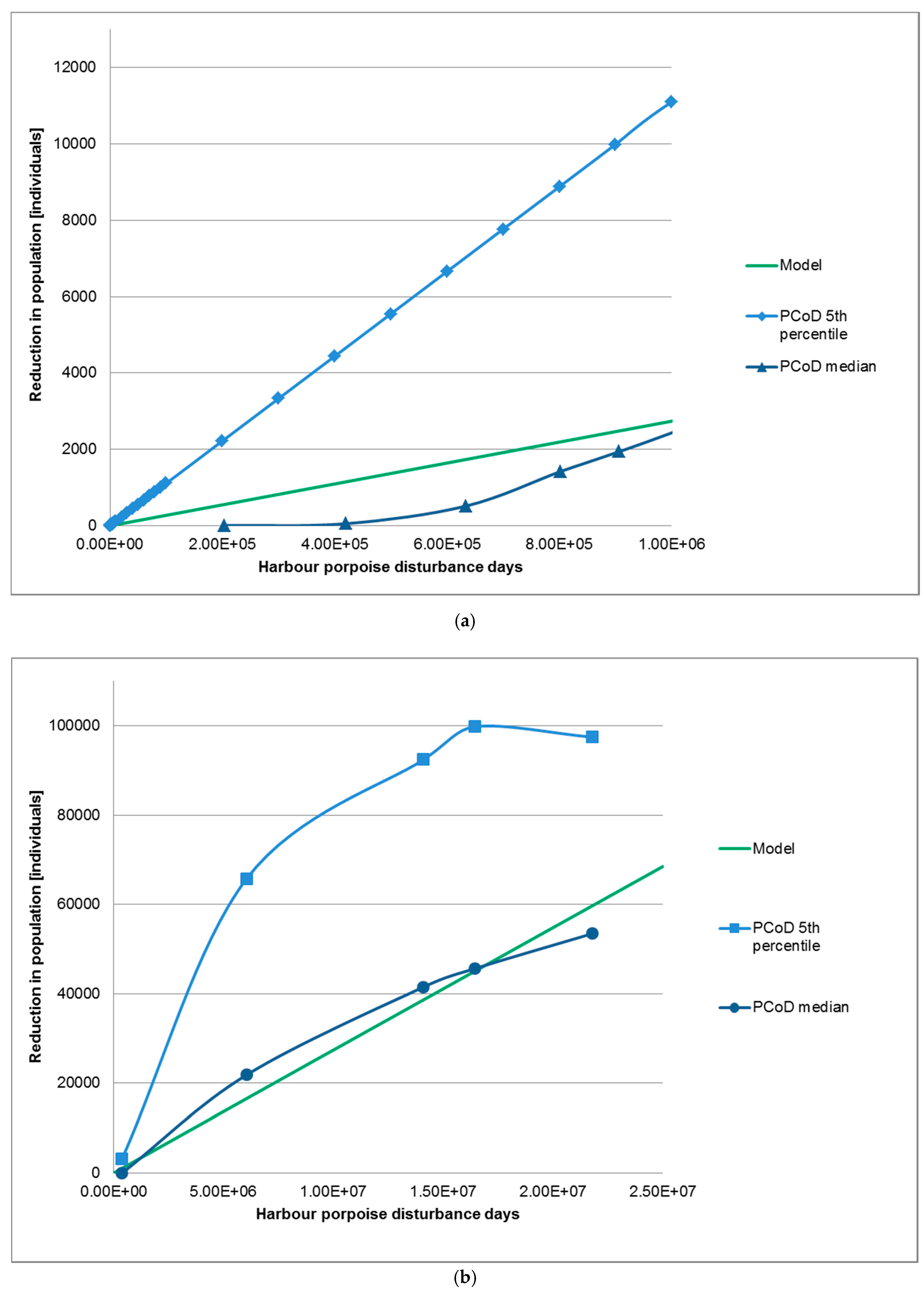
To verify whether our approach is a sensible simplification of the PCoD model or not, we compared the result with the results presented by Heinis et al. [42]. They present their results in a graph showing the harbour porpoise population reduction over harbour porpoise disturbance days (HPDD), for both a small and large vulnerable subpopulation (with smaller and larger HPDD numbers, respectively). These vulnerable sub-populations represent the part of the total population that may be affected, because it is likely that not the same individuals are affected each day. We compare both the 5th percentile (worst-case) and the median values that are shown in their results.
2.4. Expansion to other Cetacean Species
Although the characterization factor, as described in Section 2.2, was initially constructed for the impacts from noise pollution on harbour porpoises, we expanded it to other cetaceans in the North Sea. Potentially, it can be expanded also to other marine mammals in the North Sea. The species specific parameters (i) are: the avoidance area Aavoidance,i (corresponding to the species specific threshold for avoidance behaviour), the population density , and the total population in the North Sea . When all the species-specific characterization factors are calculated, the final endpoint can be obtained by taking the average of these, e.g., by taking the sum of the characterization factors and dividing by the number of cetacean species, giving equal weight to all species. This is one of several proposed aggregation options [63] and an appropriate choice, since we lack information on the vulnerability of the covered species and cover only one taxon (marine mammals).
2.4.1. Threshold Values
An overview of observed behavioural responses in different studies from several cetacean species to different sound levels, coming from the three different sound types, is presented by Southall et al. [16]. They ranked these responses by severity on a scale from 1 to 9, with 5 and up being defined as avoidance behaviour [16,42]. Southall et al. [16] grouped the different marine mammal species according to their hearing capabilities. The three cetacean functional hearing groups and their auditory bandwidth are: low-frequency (7 Hz to 22 kHz), mid-frequency (150 Hz to 160 kHz), and high-frequency (200 Hz to 180 kHz). We determined the threshold level for each functional hearing group by taking the average of the sound levels for which a behavioural response of a severity larger than 5 has been observed.
The threshold levels as described above are based on observed behaviour to different sources of noise. To make these more relevant for noise from pile-driving, we used frequency-weighting. As mentioned in Section 2.2.2, the study by Southall et al. [16] provides a method to apply frequency-weighting to a sound spectrum. The weighting functions deemphasize frequencies that are near the lower and upper frequency ends of the estimated hearing range of the functional hearing groups, as a function of the sensitivity to those frequencies [16]. The frequency-weighting curves for the cetacean functional hearing groups can be found in the Supplementary Materials. This weighting was applied to the sound spectrum of the PAWP pile-driving as presented by Heinis et al. [42]. This difference in the total broadband SEL due to the weighting was accounted for in the threshold levels of the three cetacean functional hearing groups.
2.4.2. Abundance and Population Density Data
We use abundance data of cetaceans in the European Atlantic shelf waters from a study by Hammond et al. [64], which presents data for five different cetaceans: Minke whale (Balaenoptera acutorostrata), bottlenose dolphin (Tursiops truncatus), whitebeaked dolphin (Lagenorhynchus albirostris), short-beaked common dolphin (Delphinus delphis), and the harbour porpoise (Phocoena phocoena). The data used can be found in the Supplementary Materials. The minke whale belongs to the low-frequency hearing group, the dolphins to the mid-frequency hearing group, and the porpoise to the high-frequency hearing group. Population densities and abundances are given for different segments of the European Atlantic shelf. To obtain total values for the North Sea, we only used the data of the segments that together make up the North Sea. For the local calculations, we used only the segment of the Dutch continental shelf, where the PAWP was constructed. Unfortunately, all measurements were taken during summer and so no seasonal variability is taken into account here and values are calculated only for the summer season, using Equations (2) and (3).
2.5. Case-Study
To compare the impacts of noise pollution, based on the present approach, with other impact categories, and to see if the order of magnitude of these results are reasonable, we applied the developed characterization factor in a small case study. A study by Arvesen et al. [65] quantified the impacts from the construction phase of an offshore wind farm of similar size as the PAWP, for which we now added the impacts of noise pollution. The input values used for this comparison are shown in Table 1.
The number of disturbance days comes from the first scenario by Heinis et al. [42], where a total of 580 disturbance days were assumed over a construction period of 5 years, in which two wind farms were constructed. By splitting this value by two wind farms and a 5-year duration, we obtain the disturbance per year for one wind farm.
The impacts are presented as midpoints in the study by Arvesen et al. [65]. Each impact category has its own unit (e.g., CO2-eq for climate change and 1,4DCB-eq for toxicity impacts) and therefore comparisons across impact categories are impossible. We converted all the results of Arvesen et al. [65] to endpoints (PDF values for all impact categories) to allow such a comparison. This was done by using the midpoint-to-endpoint conversion factors for the different impact categories from the ReCiPe method [61]. Only the impact categories that have an impact on the AoP of ecosystem quality were taken into account for this comparison.
3. Results
3.1. Sound Propagation
The decrease of SELs with increasing distance from the sound source, calculated using the spherical propagation loss in Equation (1), can be seen in Figure S1 in the Supplementary Materials. The range for which Ainslie and de Jong [53] recommend the spherical spreading loss relation (between 1 km and 10 km) was found to correspond to SELs between 172 dB and 152 dB. For distances smaller than 1 km, the SELs rapidly increase. For distances larger than 10 km, the SELs decrease slowly, and almost stagnate at 130 dB for distances larger than 100 km.
3.2. Verification of Approach
The results of the comparison between the results from the PCoD model and our adapted approach, as described in Section 2.2, are shown in Figure 2. Heinis et al. [42] conclude from their results that the relation between absolute reduction in population and harbour porpoise disturbance days (HPDD) is not dependent on the size of the vulnerable sub-population and that for less than 106 HPDDs the population reduction increases linearly.
Figure 2a shows that for less than one million HPDD the result from the model used in this paper also increases linearly, with a rate that closer resembles the PCoD median results than its 5th percentile results. For larger numbers of HPDD (Figure 2b), the model still closely resembles the median results from the PCoD, and mostly underestimates the reduction in population. We therefore conclude that our approach is a valid simplification of the PCoD model.
3.3. Characterization Factors
For the case study, the midpoint (affected animals.year) and endpoint CFs are calculated for the five cetacean species living in the North Sea mentioned earlier, both on a local and a regional scale. The results are shown in Table 2. The results of the species-specific parameters previously used to calculate these CFs can be found in the Supplementary Materials.
3.4. Comparison with other Impact Categories
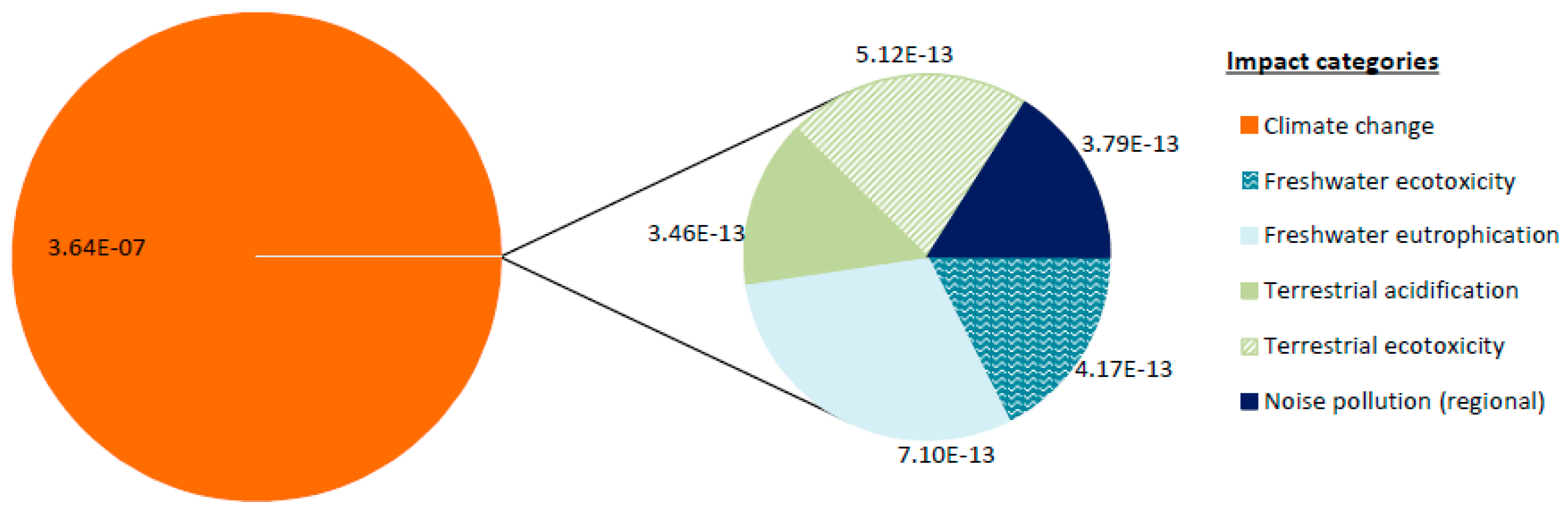
A comparison of the regional endpoint for noise pollution to the other impact categories assessed by Arvesen et al. [65] is shown in Figure 3. As described in Section 2.5, we transformed the midpoint results of Arvesen et al. [65] to endpoints for the sake of allowing a comparison across impact categories. The impact of climate change calculated by Arvesen et al. [65], which represents 99.9% of the total environmental impact, is depicted on the left. The other impacts are expanded on the right to show their relative relevance.
4. Discussion
4.1. Choice of Impact Pathway
Offshore wind farms are known to have negative impacts on the cultural, provisioning, and supporting services of marine ecosystems [66]. Most environmental studies focus on the operational phase of offshore wind, finding both negative and positive impacts for different species (mammals, birds, fish, etc.) [66]. Studies that assess the impacts of the construction phase are only available for mammals and birds, but show mostly negative impacts [66]. Marine mammals that are near to a construction site where pile-driving takes place are found to be subjected to temporary hearing loss, increased stress levels, and avoidance behaviour leading to habitat loss [66], which can potentially affect a whole population, and subsequently the marine ecosystem [67]. It must be noted that pile-driving is classified as a multiple pulse sound source [16]. The method proposed here may not be applicable to single-pulse sounds such as single explosions, or non-pulse sounds such as acoustic deterrent devices. However, it is adequate for noise from the same sound type, such as sequential airguns and certain sonars.
Cetaceans were chosen as the species of interest for this paper, partly due to the amount of literature available on the effect of noise pollution on them (see e.g., also [44,45,46,47,48,49]). While research has been undertaken on a range of marine species, the focus has mainly been on cetaceans. This may be related to “the inherent appeal of these charismatic megafauna to the general public”, as Wright [68] puts it. This may therefore falsify the impression we get of which species are most affected. In addition, taking the most sensitive species as an indicator for the whole ecosystem may cause an overestimation of the total impact.
Although the study location was not a relevant factor in the decision-making, it is important to note that the North Sea is an area of interest regarding noise pollution in general. Most of the ocean noise pollution comes from offshore industry in coastal areas, which are overall greatly affected by human activities [69]. Simultaneously, this is where most of marine life is located. Hence, most of the impacts of marine noise pollution are expected to occur in coastal areas. In addition, the North Sea is defined as a large marine ecosystem (LME) by the US National Oceanic and Atmospheric Administration (NOAA) to identify areas of the oceans for conservation purposes [70], and can therefore be said to be of appropriate scale for assessing the impacts of noise on marine ecosystems. A similar approach (with LMEs) was adopted for marine coastal eutrophication in an LCA context [71].
4.2. Characterization Factor Development
4.2.1. Sound Propagation Model
Sound propagation was calculated assuming only a loss due to spherical propagation, which is a significant simplification that we are aware of. We regard the development of the CFs using this simplified sound propagation approach as a first attempt with the aim to test whether this impact category bears any significance at all. We conclude that the impact is indeed relevant (as seen in Figure 3 in comparison with other impact categories) and therefore stress the importance of going beyond this first, simplistic representation of sound propagation models in the further development of the model. Although this is a large simplification of reality, for the case of the PAWP (which Heinis et al. [42] assume to be a basis for all noise estimations of monopile driving in the North Sea), it is a valid one: Ainslie and de Jong [53], including noise measurements from other pile-driving activities at several distances between 1 km and 10 km, found a good fit for spherical propagation of the loss estimation. They do, however, also note that this relation is only valid for the specific frequency bandwidth and sound type of pile-driving, and do not recommend to use it for distances beyond the range of their measurements [53]. Models using cylindrical spreading instead of a spherical one should be investigated for further model development, especially for activities taking place in shallow waters.
Since the sound propagation calculation is only validated by measurements over a small range of distance (1 km to 10 km), it probably only holds for a small range of sound levels (172 dB to 152 dB). For smaller and larger distances, the SEL becomes highly sensitive. For calculations of avoidance areas for threshold levels outside this range, a high uncertainty must be taken into consideration. However, simplifications such as these are not uncommon in LCA. Each impact category struggles with its own set of required simplifications, for example land use uses a (often very simple) species-area relationship, which does not fully capture the complexity of the “real” nature [72], even though development for increasing the complexity are also on-going.
4.2.2. Disturbance Days
The disturbance days parameter can be used in several ways. Heinis et al. [42] assume in their study that the effects of a disturbance that lasts for only a part of the day continues for at least one whole day (24 h) and this is also the assumption we make here. Some field studies on harbour porpoises, however, observed that porpoises returned to their normal behaviour as soon as the stressor was interrupted, while on other occasions the porpoises stayed away for up to three days (72 h) after the exposure [42,44]. More specific data on harbour porpoise behaviour are required for this variable, as well as a construction scheme of the offshore power plant; if the construction takes place on consecutive days, the calculated impact depends less on the number of disturbance days.
4.2.3. Endpoint Characterization Factor
Normalizing the number of affected animals by the total population within an area of interest to obtain a fraction of species (temporarily) disappeared makes the characterization factor highly dependent on the scale of the area of interest. A larger area of interest will result in a smaller fraction of potentially affected animals if the total population is larger. When comparing the results with the ones of the offshore wind park we get an overview of the magnitude of the impact. Losses caused by local to regional impacts can be expected to be larger than generic (global CFs) impacts—it is easier to cause a local disappearance than a global extinction of a species. This issue of scale (local vs. regional vs. global) is a common challenge within LCA, and it should be dealt with carefully and consistently across impact categories [73].
Moreover, when local distribution data is not available, only a regional impact can be calculated, by assuming the population density to be the same for the whole regional ecosystem. The density and abundance are both directly related to the total area of the ecosystem. The characterization factor then, essentially, becomes dependent only on the disturbance days and the ratio of avoidance area over total area of the ecosystem of interest.
The proposed characterization factor assumes a ratio of 1:1 between the potentially affected animals and potentially disappeared animals, i.e., the animals that avoid the area disappear for the duration of the disturbance. This is a necessary simplification due to lack of data. The relationship between the potentially affected animals and the loss of animals is a topic of debate within LCA, and it is not uncommon to use a ratio of 1:1 as an assumption [73]. It does, however, not include the cumulative effects of multiple exposures to noise pollution. Although LCA does not currently include cumulative effects, we believe that, for the case of noise pollution especially, this is something that should be looked into. Not much quantitative data exists on this aspect, but for the PCoD model, an expert elicitation was used to provide a curve that shows the relationship between the number of disturbance days and the effect on survival or fertility of the individual [74,75]. These curves, however, are only available for a small number of species, and have a high uncertainty due to a lack of consensus between the experts [42].
4.3. Application to other Cetacean Species
The avoidance area for low-frequency cetaceans (shown in Table S3 in the Supplementary Materials) is very large. This can be explained by the fact that the threshold SEL is far outside the validity range of the sound propagation calculation (see Section 4.2.1). The threshold SEL for high-frequency cetaceans is also outside that range. The avoidance area, however, is of the same order of magnitude as that of harbour porpoises as calculated with the AQUARIUS model [42].
It must be noted that, although our approach for the harbour porpoise was evaluated and found reasonable, it is not necessarily expandable to other species. Harbour porpoises are known to be highly sensitive to disturbances [76]. Because of their small size and high metabolic rate, they feed at high rates year-round; thus, if unable to feed for 3–4 days, starvation may occur [42]. Applying the same approach for all (and mostly larger and less sensitive) cetacean species is likely to overestimate the total impact. This could be taken into account in the ratio between the potentially affected fraction (PAF) and the potentially disappeared fraction (PDF), by taking another conversion relationship than a 1:1 relationship, as discussed in the previous section.
From the sound spectrum of a pile strike, it can be seen that the frequency-weighting curves have most effect for the mid- and high-frequency hearing groups (Figure S3). The frequency-weighting has only been used to include the sensitivity of a species to different frequencies, but has not been included in the sound propagation modelling. This may be something to look into in the future, since propagation loss is dependent on the frequency of sound [53].
4.4. Case-Study
When calculated with local level population densities, the endpoint for the minke whale and the harbour porpoise are of the same order of magnitude. Although the minke whale has a significant avoidance area, the ratio between animal density and total population is small. As discussed before, this avoidance area may most likely be invalid, due to the avoidance distance being outside of the valid range of the sound propagation model used. For the regional endpoint, however, this ratio does not affect the result and the large avoidance area results in an endpoint that is one order of magnitude larger than for the harbour porpoise. The dependency of the regional endpoint on the avoidance area can also be seen for the mid-frequency cetaceans, which are all equal due to an equal avoidance area. The mid-frequency cetaceans also have lower endpoints overall, due to the lower local animal density and avoidance area. For the white-beaked dolphin, the local animal density is zero and therefore so is the local endpoint. The higher total endpoint for the regional level can be explained by the significantly higher regional endpoint of the minke whale.
Nearly all (99.9%) of the impact on ecosystem quality (Figure 3) comes from the climate change category. This is as expected, since it is a global-scale impact and is usually multiple orders of magnitude larger than other impact categories and is time-integrated over 100 years. When comparing the noise pollution impact to the other categories, it can be seen that these are of the same order of magnitude, with no significant differences. It must be noted, however, that one should be careful when comparing different impact categories and different ecosystems (terrestrial, freshwater, marine) because of the characteristics of the ecosystems and the scales (regional and global) at which the impacts are calculated, as was also discussed in the previous section.
5. Conclusions
The approach described in this paper is a first attempt for the inclusion of noise pollution in marine ecosystems in an LCA framework. Although only applied here on one impact pathway and only for the North Sea, it shows potential for other pathways and regions as well. Because of data limitations, many assumptions will have to be made for that and uncertainties will remain. In addition, better and more sophisticated noise propagation models will need to be investigated (e.g., cylindrical spreading vs. spherical spreading) and the choice and number of species considered (e.g., minke whales may be more sensitive than thought and also have a high CF value in our study) will need to be improved. However, we believe it is better to have at least some quantification of impacts in the noise pollution impact category in LCA than having none at all. The impacts from noise pollution on marine ecosystems have long been overlooked, but cannot be ignored any longer. Our approach contributes a valuable first step towards reducing this ignorance.
Supplementary Materials
The following are available online at www.mdpi.com/2071-1050/9/7/1138/s1. There are two documents available as Supplementary Materials: A pdf file containing information on the choice of impact pathway, the sound propagation model we used, the abundance data for cetaceans in the North Sea, and the frequency weighting curves for the different functional hearing groups of cetaceans; and an Excel file for details on the 23 mentioned studies that were used for choosing an impact pathway.
Acknowledgments
We thank John S. Woods for English checking and helpful comments during the writing process.
Author Contributions
Heleen Middel and Francesca Verones conceived the research; Heleen Middel performed the analyses and calculated the model; Heleen Middel and Francesca Verones wrote the paper.
Conflicts of Interest
The authors declare no conflict of interest.
References
- Costanza, R. The ecological, economic, and social importance of the oceans. Ecol. Econ. 1999, 31, 199–213. [Google Scholar] [CrossRef]
- The State of World Fisheries and Aquaculture. Fisheries and Aquaculture Department, Food and Agriculture Organization; FAO: Rome, Italy, 2014. [Google Scholar]
- HLPE. Sustainable Fisheries and Aquaculture for Food Security and Nutrition; High Level Panel of Experts of Food Security and Nutrition of the Committee on World Food Security: Rome, Italy, 2014; Available online: http://www.fao.org/3/a-i3844e.pdf (accessed on 27 June 2017).
- Tanzer, J.; Phua, C.; Jeffries, B.; Lawrence, A.; Gonzales, A.; Gamblin, P.; Roxburgh, T. Living Blue Planet Report Species, Habitats and Human Well-Being; WWF International: Gland, Switzerland, 2015. [Google Scholar]
- IPCC. Climate Change 2013: The Physical Science Basis; Contribution of Working Group I to the Fifth Assessment Report of the IPCC; Cambridge University Press: Cambridge, UK; New York, NY, USA, 2013. [Google Scholar]
- BCG. BCG Economic Valuation: Methodology and Sources. Reviving the Ocean Economy: The Case for Action; Boston Consulting Group, Global Change Institute and WWF International: Gland, Switzerland, 2015. [Google Scholar]
- Wiber, M.G.; Young, S.; Wilson, L. Impact of Aquaculture on Commercial Fisheries: Fishermen’s Local Ecological Knowledge. Hum. Ecol. 2012, 40, 29–40. [Google Scholar] [CrossRef]
- Wysocki, L.E.; Davidson, J.W.; Smith, M.E.; Frankel, A.S.; Ellison, W.T.; Mazik, P.M.; Popper, A.N.; Bebak, J. Effects of aquaculture production noise on hearing, growth, and disease resistance of rainbow trout Oncorhynchus mykiss. Aquaculture 2007, 272, 687–697. [Google Scholar] [CrossRef]
- Tournadre, J. Anthropogenic pressure on the open ocean: The growth of ship traffic revealed by altimeter data analysis. Geophys. Res. Lett. 2014, 41, 7924–7932. [Google Scholar] [CrossRef]
- Maribus. World Ocean Review 3: Living with Oceans: Marine Resources—Opportunities and Risks; Maribus GmbH: Hamburg, Germany, 2014. [Google Scholar]
- McCauley, R.D.; Fewtrell, J.; Popper, A.N. High intensity anthropogenic sound damages fish ears. J. Acoust. Soc. Am. 2003, 113, 638–642. [Google Scholar] [CrossRef] [PubMed]
- Kunc, H.P.; McLaughlin, K.E.; Schmidt, R. Aquatic noise pollution: Implications for individuals, populations, and ecosystems. Proc. R. Soc. B 2016, 283. [Google Scholar] [CrossRef] [PubMed]
- Hawkins, A.D.; Pembroke, A.E.; Popper, A.N. Information gaps in understanding the effects of noise on fishes and invertebrates. Rev. Fish Biol. Fish. 2015, 25, 39–64. [Google Scholar] [CrossRef]
- Slabbekoorn, H.; Bouton, N.; van Opzeeland, I.; Coers, A.; ten Cate, C.; Popper, A.N. A noisy spring: The impact of globally rising underwater sound levels on fish. Trends Ecol. Evol. 2010, 25, 419–427. [Google Scholar] [CrossRef] [PubMed]
- Popper, A.N. Effects of Anthropogenic Sounds on Fishes. Fisheries 2003, 28, 24–31. [Google Scholar] [CrossRef]
- Southall, B.L.; Bowles, A.E.; Ellison, W.T.; Finneran, J.J.; Gentry, R.L.; Greene, C.R.; Kastak, D.; Ketten, D.R.; Miller, J.H.; Nachtigall, P.E.; et al. Marine Mammal Noise Exposure Criteria: Initial Scientific Recommendations. Aquat. Mamm. 2007, 33, 411–414. [Google Scholar] [CrossRef]
- Warner, R.M. Protecting the diversity of the depths: Environmental regulation of bioprospecting and marine scientific research beyond national jurisdiction. Ocean Yearb. 2008, 22, 411–443. [Google Scholar] [CrossRef]
- Romano, T.A.; Keogh, M.J.; Kelly, C.; Feng, P.; Berk, L.; Schlundt, C.E.; Carder, D.A.; Finneran, J.J. Anthropogenic sound and marine mammal health: Measures of the nervous and immune systems before and after intense sound exposure. Can. J. Fish. Aquat. Sci. 2004, 61, 1124–1134. [Google Scholar] [CrossRef]
- Morton, A. Displacement of Orcinus orca (L.) by high amplitude sound in British Columbia, Canada. ICES J. Mar. Sci. 2002, 59, 71–80. [Google Scholar] [CrossRef]
- Wysocki, L.E.; Dittami, J.P.; Ladich, F. Ship noise and cortisol secretion in European freshwater fishes. Biol. Conserv. 2006, 128, 501–508. [Google Scholar] [CrossRef]
- Sarà, G.; Dean, J.; D’Amato, D.; Buscaino, G.; Oliveri, A.; Genovese, S.; Ferro, S.; Buffa, G.; Martire, M.; Mazzola, S. Effect of boat noise on the behaviour of bluefin tuna Thunnus thynnus in the Mediterranean Sea. Mar. Ecol. Prog. Ser. 2007, 331, 243–253. [Google Scholar] [CrossRef]
- Parente, C.L.; de Araújo, J.P.; de Araújo, M.E. Diversity of cetaceans as tool in monitoring environmental impacts of seismic surveys. Biot. Neotrop. 2007, 7. [Google Scholar] [CrossRef]
- Fernández, A.; Edwards, J.F.; Rodríguez, F.; Espinosa de los Monteros, A.; Herráez, P.; Castro, P.; Jaber, J.R.; Martín, V.; Arbelo, M. ‘Gas and fat embolic syndrome’ involving a mass stranding of beaked whales (family Ziphiidae) exposed to anthropogenic sonar signals. Vet. Pathol. 2005, 42, 446–457. [Google Scholar] [CrossRef] [PubMed]
- International Whaling Commission. Report of the Scientific Committee. J. Cetacean Res. Manag. 2015, 16. Available online: https://archive.iwc.int/?r=3436&k=4173fd68bc (accessed on 27 June 2017).
- International Whaling Commission. Report of the Scientific Committee. J. Cetacean Res. Manag. 2012, 13. Available online: https://archive.iwc.int/?r=2126&k=e5974c39c4 (accessed on 27 June 2017).
- Hellweg, S.; Milà i Canals, L. Emerging approaches, challenges and opportunities in life cycle assessment. Science 2014, 344, 1109–1113. [Google Scholar] [CrossRef] [PubMed]
- ISO 14044. Environmental Management—Life Cycle Assessment—Requirements and Guidelines (ISO14044:2006); British Standards Institute: London, UK, 2006. [Google Scholar]
- Pennington, D.W.; Potting, J.; Finnveden, G.; Lindeijer, E.; Jolliet, O.; Rydberg, T.; Rebitzer, G. Life cycle assessment Part 2: Current impact assessment practice. Environ. Int. 2004, 30, 721–739. [Google Scholar] [CrossRef] [PubMed]
- Jolliet, O.; Müller-Wenk, R.; Bare, J.; Brent, A.; Goedkoop, M.; Heijungs, R.; Itsubo, N.; Peña, C.; Pennington, D.; Potting, J.; et al. The LCIA midpoint-damage framework of the UNEP/SETAC life cycle initiative. Int. J. Life Cycle Assess. 2004, 9, 394–404. [Google Scholar] [CrossRef]
- Hauschild, M.Z.; Huijbregts, M.A.J. Life Cycle Impact Assessment; Springer: Dordrecht, The Netherlands, 2015. [Google Scholar]
- Cucurachi, S.; Heijungs, R.; Ohlau, K. Towards a general framework for including noise impacts in LCA. Int. J. Life Cycle Assess. 2012, 17, 471–487. [Google Scholar] [CrossRef] [PubMed]
- Hollander, A.E.; Melse, J.M.; Kramers, P.G. An aggregate public health indicator to represent the impact of multiple environmental exposures. Epidemiol. Baltim. 1999, 10, 606–617. [Google Scholar] [CrossRef]
- Müller-Wenk, R. A method to include in LCA road traffic noise and its health effects. Int. J. Life Cycle Assess. 2004, 9, 76–85. [Google Scholar] [CrossRef]
- Peng, C.; Zhao, X.; Liu, G. Noise in the Sea and Its Impacts on Marine Organisms. Int. J. Environ. Res. Public Health 2015, 12, 12304–12323. [Google Scholar] [CrossRef] [PubMed]
- Tyack, P.L. Implications for marine mammals of large-scale changes in the marine acoustic environment. J. Mamm. 2008, 83, 549–558. [Google Scholar] [CrossRef]
- Richardson, W.J.; Greene, C.R.; Malme, C.I.; Thomson, D.H. Marine Mammals and Noise; Academic Press: Cambridge, MA, USA, 2013. [Google Scholar]
- Nowacek, D.P.; Thorne, L.H.; Johnston, D.W.; Tyack, P.L. Responses of cetaceans to anthropogenic noise. Mamm. Rev. 2007, 37, 81–115. [Google Scholar] [CrossRef]
- NRC. Ocean Noise and Marine Mammals; National Academies Press: Washington, DC, USA, 2003. [Google Scholar]
- Erbe, C. Underwater Acoustics: Noise and the Effects on Marine Mammals, a Pocket Handbook; Jasco Applied Sciences: Halifax, NS, Canada, 2011. [Google Scholar]
- Cox, T.M.; Ragen, T.J.; Read, A.J.; Vos, E.; Baird, R.W.; Balcomb, K.; Barlow, J.; Caldwell, J.; Cranford, T.; Crum, L.; et al. Understanding the impacts of anthropogenic sound on beacked whales. J. Cetacean Res. Manag. 2006, 7, 177–187. [Google Scholar]
- Weilgart, L. The impacts of anthropogenic ocean noise on cetaceans and implications for management. Can. J. Zool. 2007, 85, 1091–1116. [Google Scholar] [CrossRef]
- Heinis, F.; de Jong, C.A.F. Cumulative Effects of Impulsive Underwater Sound on Marine Mammals; TNO Report; TNO: The Hague, The Netherlands, 2015. [Google Scholar]
- King, S.L.; Schick, R.S.; Donovan, C.; Booth, C.G.; Burgman, M.; Thomas, L.; Harwood, J. An interim framework for assessing the population consequences of disturbance. Methods Ecol. Evol. 2015, 6, 1150–11585. [Google Scholar] [CrossRef]
- Brandt, M.J.; Diederichs, A.; Betke, K.; Nehls, G. Responses of harbour porpoises to pile driving at the Horns Rev II offshore wind farm in the Danish North Sea. Mar. Ecol. Prog. Ser. 2011, 421, 205–216. [Google Scholar] [CrossRef]
- Dähne, M.; Gilles, A.; Lucke, K.; Peschko, V.; Adler, S.; Krügel, K.; Sundermeyer, J.; Siebert, U. Effects of pile-driving on harbour porpoises (Phocoena phocoena) at the first offshore wind farm in Germany. Environ. Res. Lett. 2013, 8, 1–16. [Google Scholar] [CrossRef]
- Tougaard, J.; Carstensen, J.; Teilmann, J.; Skov, H.; Rasmussen, P. Pile driving zone of responsiveness extends beyond 20 km for harbor porpoises (Phocoena phocoena (L.)). J. Acoust. Soc. Am. 2013, 126, 11–14. [Google Scholar] [CrossRef] [PubMed]
- Tougaard, J.; Kyhn, L.A.; Amundin, M.; Wennerberg, D.; Bordin, C. Behavioral Reactions of Harbor Porpoise to Pile-Driving Noise. In The Effects of Noise on Aquatic Life; Popper, A.N., Hawkins, A., Eds.; Springer: New York, NY, USA, 2012; pp. 277–280. [Google Scholar]
- Tougaard, J.; Wright, A.J.; Madsen, P.T. Cetacean noise criteria revisited in the light of proposed exposure limits for harbour porpoises. Mar. Pollut. Bull. 2015, 90, 196–208. [Google Scholar] [CrossRef] [PubMed]
- New, L.F.; Clark, J.S.; Costa, D.P.; Fleishman, E.; Hindell, M.A.; Klanjcek, T.; Lusseau, D.; Kraus, S.; McMahon, C.R.; Robinson, P.W.; et al. Using short-term measures of behaviour to estimate long-term fitness of southern elephant seals. Mar. Ecol. Prog. Ser. 2013, 496, 99–108. [Google Scholar] [CrossRef]
- Harwood, J.; King, S.L. The Sensitivity of UK Marine Mammal Populations to Marine Renewables Developments; Natural Environment Research Council (NERC): Swindon, UK, 2014. [Google Scholar]
- National Research Council. Marine Mammal Populations and Ocean Noise: Determining When Noise Causes Biologically Significant Effects; The National Academy Press: Washington, DC, USA, 2005.
- Matthews, M.-N.R.; Zykov, M. Underwater Acoustic Modeling of Construction Activities: Marine Commerce South Terminal in New Bedford, MA; LCC: Boston, MA, USA, 2012. [Google Scholar]
- Ainslie, M.A.; de Jong, C.A.F.; Dol, H.S.; Blacquière, G.; Marasini, C. Assessment of Natural and Anthropogenic Sound Sources and Acoustic Propagation in the North Sea; TNO: The Hague, The Netherlands, 2009. [Google Scholar]
- De Jong, C.A.F.; Ainslie, M.A. Underwater Sound due to Piling Activities for Prinses Amaliawindpark; TNO: The Hague, The Netherlands, 2012. [Google Scholar]
- Huijbregts, M.A.J.; Hellweg, S.; Hertwich, E. Do We Need a Paradigm Shift in Life Cycle Impact Assessment? Environ. Sci. Technol. 2011, 45, 3833–3834. [Google Scholar] [CrossRef] [PubMed]
- U.S. Navy. Atlantic Fleet Active Sonar Traning Environmental Impact Statement; Naval Facilities Engineering Command: Atlantic, NJ, USA, 2008.
- Parsons, E.C.M.; Dolman, S.J.; Wright, A.J.; Rose, N.A.; Burns, W.C.G. Navy sonar and cetaceans: Just how much does the gun need to smoke before we act? Mar. Pollut. Bull. 2008, 56, 1248–1257. [Google Scholar] [CrossRef] [PubMed]
- Bronštejn, I.N.; Semendjaev, K.A.; Musiol, G.; Mühlig, H. Taschenbuch der Mathematik, 1. Auflage; Verlag Harri Deutsch: Frankfurt, Germany, 1993. [Google Scholar]
- Geelhoed, S.; Scheidat, M.; Aarts, G.; van Bemmelen, R.; Janinhoff, N.; Verdaat, H.; Witte, R. Shortlist Masterplan Wind Aerial Surveys of Harbour Porpoises on the Dutch Continental Shelf; Institute for Marine Resources and Ecosystem Studies: Wageningen, The Netherlands, 2011; Available online: https://tethys.pnnl.gov/publications/shortlist-masterplan-wind-aerial-surveys-harbour-porpoises-dutch-continental-shelf (accessed on 27 June 2017).
- Goedkoop, M.; Spriensma, R. The Eco-Indicator 99: A Damage Oriented Method for Life Cycle Impact Assessment—Methodology Report and Annex; Pré Consultants B.V.: Amersfoort, The Netherlands, 1999. [Google Scholar]
- Goedkoop, M.; Heijungs, R.; Huijbregts, M.A.J.; De Schryver, A.; Struijs, J.; Van Zelm, R. ReCiPe 2008: A Life Cycle Impact Assessment Method Which Comprises Harmonised Category Indicators at the Midpoint and Endpoint Level, 1st ed.; Ruimte en Milieu, Ministerie van Volkshuisvesting, Ruimtelijke Ordening en Milieubeheer, TNO: The Hague, The Netherlands, 2009. [Google Scholar]
- Verones, F.; Hellweg, S.; Azevedo, L.B.; Chaudhary, A.; Cosme, N.; Fantke, P.; Goedkoop, M.; Hauschild, M.Z.; Laurent, A.; Mutel, C.L.; et al. LC-IMPACT Version 0.5: A Spatially Differentiated Life Cycle Impact Assessment Approach. 2016. Available online: http://www.lc-impact.eu/downloads/documents/LC-Impact_report_SEPT2016_20160927.pdf (accessed on 28 April 2017).
- Verones, F.; Huijbregts, M.A.J.; Chaudhary, A.; de Baan, L.; Koellner, T.; Hellweg, S. Harmonizing the Assessment of Biodiversity Effects from Land and Water Use within LCA. Environ. Sci. Technol. 2015, 49, 3584–3592. [Google Scholar] [CrossRef] [PubMed]
- Hammond, P.S.; Macleod, K.; Berggren, P.; Leopold, M.F.; Scheidat, M. Cetacean abundance and distribution in European Atlantic shelf waters to inform conservation and management. Biol. Conserv. 2013, 164, 107–122. [Google Scholar] [CrossRef]
- Arvesen, A.; Birkeland, C.; Hertwich, E.G. The Importance of Ships and Spare Parts in LCAs of Offshore Wind Power. Environ. Sci. Technol. 2013, 47, 2948–2956. [Google Scholar] [CrossRef] [PubMed]
- Papathanasopoulou, E.; Beaumont, N.; Hooper, T.; Nunes, J.; Queirós, A.M. Energy systems and their impacts on marine ecosystem services. Renew. Sustain. Energy Rev. 2015, 52, 917–926. [Google Scholar] [CrossRef]
- Dähne, M.; Peschko, V.; Gilles, A.; Lucke, K.; Adler, S.; Ronnenberg, K.; Siebert, U. Marine mammals and windfarms: Effects of alpha ventus on harbour porpoises. In Ecological Research at the Offshore Windfarm Alpha Ventus; Federal Maritime and Hydrographic Agency, Federal Ministry for the Environment, Nature Conservation and Nuclear Safety, Eds.; Springer Fachmedien Wiesbaden: Wiesbaden, Germany, 2014. [Google Scholar]
- Wright, A.J. Reducing Impacts of Human Ocean Noise on Cetaceans: Knowledge Gap Analysis and Recommendations; WWF Global Arctic Programme: Ottawa, ON, Canada, 2014. [Google Scholar]
- Kaiser, M.J.; Attrill, M.J. Marine Ecology: Processes, Systems, and Impacts, 2nd ed.; Oxford University Press: New York, NY, USA, 2011. [Google Scholar]
- NOAA. The Large Marine Ecosystem Approach to the Assessment and Management of Coastal Ocean Waters. Large Marine Ecosystems of the World, 2016. Available online: http://www.lme.noaa.gov/ (accessed on 5 September 2016).
- Cosme, N.; Jones, M.C.; Cheung, W.W.L.; Larsen, H.F. Spatial differentiation of marine eutrophication damage indicators based on species density. Ecol. Indic. 2017, 73, 676–685. [Google Scholar] [CrossRef]
- De Baan, L.; Alkemade, R.; Koellner, T. Land use impacts on biodiversity in LCA: A global approach. Int. J. Life Cycle Assess. 2013, 18, 1216–1230. [Google Scholar] [CrossRef]
- Curran, M.; de Baan, L.; De Schryver, A.; Van Zelm, R.; Hellweg, S.; Koellner, T.; Sonnemann, G.; Huijbregts, M.A.J. Toward Meaningful End Points of Biodiversity in Life Cycle Assessment. Environ. Sci. Technol. 2011, 45, 70–79. [Google Scholar] [CrossRef] [PubMed]
- Donovan, C.; Harwood, J.; King, S.; Booth, C.; Caneco, B.; Walker, C. Expert Elicitation Methods in Quantifying the Consequences of Acoustic Disturbance from Offshore Renewable Energy Developments. In The Effects of Noise on Aquatic Life II; Popper, A.N., Hawkins, A., Eds.; Springer: New York, NY, USA, 2016. [Google Scholar]
- Harwood, J.; King, S.; Schick, R.; Donovan, C.; Booth, C. A Protocol for Implementing the Interim Population Consequences of Disturbance (PCOD) Approach: Quantifying and Assessing the Effects of UK Offshore Renewable energy Developments on Marine Mammal Populations. Report Number SMRUL-TCE-2013-014. Available online: http://www.gov.scot/Resource/0044/00443360.pdf (accessed on 28 April 2017).
- Wisniewska, D.M.; Johnson, M.; Teilmann, J.; Rojano-Doñate, L.; Shearer, J.; Sveegaard, S.; Miller, L.A.; Siebert, U.; Madsen, P.T. Ultra-High Foraging Rates of Harbor Porpoises Make Them Vulnerable to Anthropogenic Disturbance. Curr. Biol. 2016, 26, 1441–1446. [Google Scholar] [CrossRef] [PubMed]
Figure 1.
Schematic flowchart for the steps of performing an LCA from the life cycle inventory to the different stages in the LCIA (midpoint levels, endpoint levels and aggregated endpoints. Note that in the endpoint impact categories only the metric relevant for ecosystem quality is given. From the aggregated endpoints (to the area of protection), only “ecosystem quality” (in red) is relevant for our purpose.
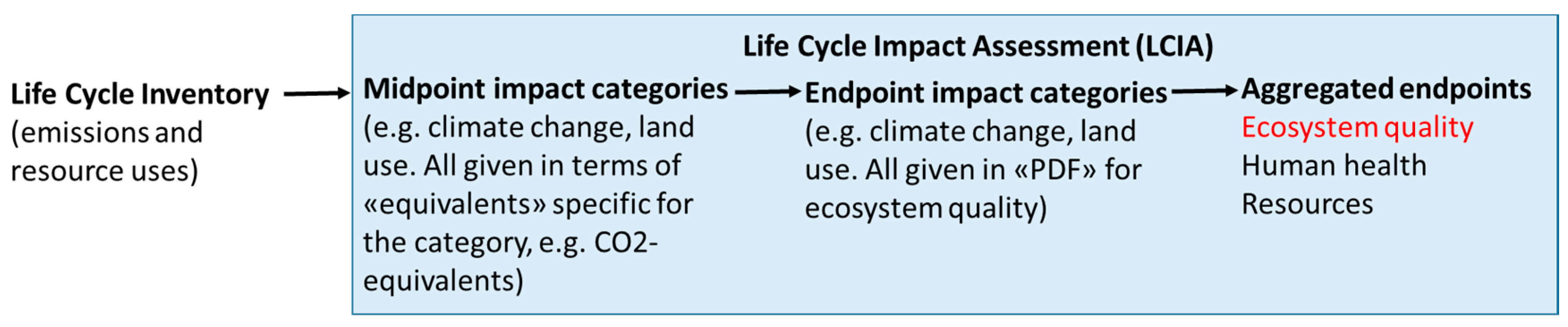
Figure 2.
(a) Absolute reduction in population over the harbour porpoise disturbance days, results from the PCoD model used by Heinis et al. [42] (median and 5th percentile values), using a vulnerable subpopulation of 30,000 harbour porpoises, and our model (in green) as described in this paper; (b) Absolute reduction in population over the harbour porpoise disturbance days, results from the PCoD model used by Heinis et al. [42] (median and 5th percentile values), using a vulnerable subpopulation of 129,329 harbour porpoises, and our model (in green) as described in this paper.

Figure 3.
Impacts from the construction phase of the offshore windfarm as described in the case study (Section 2.5), based on Arvesen et al. [65]. On the left, the total impact is shown (depicting the 99.9% coming from climate change), and, on the right, the smaller impacts are expanded. The noise pollution is shown in dark blue. The impact scores are shown in PDF.yr, for the functional unit of 1 kWh produced.


Table 1.
Input values used for the case study of an offshore wind farm.
| Parameter | Value | Unit | References |
|---|---|---|---|
| Wind farm capacity | 350 | MW | [42,65] |
| Lifetime | 20 | Years | [65] |
| Full load hours | 3000 | Hours | [65] |
| Total lifetime production | 2.10 × 10¹⁰ | kWh | Calculated |
| Disturbance days per year | 58 | Days | [42] |
| Construction time | 5 | Years | [42] |
Table 2.
Results of the case study: Midpoint and endpoint CFs for the five cetacean species, on both a local and a regional level. The local endpoint for the white-beaked data is zero, because the local population density provided in Hammond et al. [64] is zero.
Table 2.
Results of the case study: Midpoint and endpoint CFs for the five cetacean species, on both a local and a regional level. The local endpoint for the white-beaked data is zero, because the local population density provided in Hammond et al. [64] is zero.
| Functional Hearing Group | Midpoint Local [ind.yr] | Midpoint Regional [ind.yr] | Endpoint Local [PDF.yr/kWh] | Endpoint Regional [PDF.yr/kWh] |
|---|---|---|---|---|
| Low-frequency cetaceans | ||||
| Minke whale (B. acutorostrata) | 49.964 | 80.661 | 9.93 × 10⁻¹³ | 1.60 × 10⁻¹² |
| Mid-frequency cetaceans | ||||
| Bottlenose dolphin (T. truncatus) | 0.063 | 0.030 | 1.35 × 10⁻¹⁴ | 6.39 × 10⁻¹⁵ |
| Whitebeaked dolphin (L. albirostris) | 0.000 | 0.284 | 0.00 × 10 | 6.39 × 10⁻¹⁵ |
| Short-beaked common dolphin (D. delphis) | 0.793 | 0.133 | 3.84 × 10⁻¹⁴ | 6.39 × 10⁻¹⁵ |
| High-frequency cetaceans | ||||
| Harbour porpoise (Phocoena phocoena) | 280.038 | 288.518 | 2.65 × 10⁻¹³ | 2.73 × 10⁻¹³ |
| Total | 2.62 × 10⁻¹³ | 3.79 × 10⁻¹³ | ||
© 2017 by the authors. Licensee MDPI, Basel, Switzerland. This article is an open access article distributed under the terms and conditions of the Creative Commons Attribution (CC BY) license (http://creativecommons.org/licenses/by/4.0/).
Share and Cite
MDPI and ACS Style
Middel, H.; Verones, F. Making Marine Noise Pollution Impacts Heard: The Case of Cetaceans in the North Sea within Life Cycle Impact Assessment. Sustainability 2017, 9, 1138. https://doi.org/10.3390/su9071138
AMA Style
Middel H, Verones F. Making Marine Noise Pollution Impacts Heard: The Case of Cetaceans in the North Sea within Life Cycle Impact Assessment. Sustainability. 2017; 9(7):1138. https://doi.org/10.3390/su9071138
Chicago/Turabian StyleMiddel, Heleen, and Francesca Verones. 2017. "Making Marine Noise Pollution Impacts Heard: The Case of Cetaceans in the North Sea within Life Cycle Impact Assessment" Sustainability 9, no. 7: 1138. https://doi.org/10.3390/su9071138
Note that from the first issue of 2016, this journal uses article numbers instead of page numbers. See further details here.