Carbon Reduction Potential of Resource-Dependent Regions Based on Simulated Annealing Programming Algorithm

School of Economics and Management, Taiyuan University of Technology, Taiyuan 030024, China
*
Author to whom correspondence should be addressed.
Sustainability 2017, 9(7), 1161; https://doi.org/10.3390/su9071161
Submission received: 18 May 2017
/
Revised: 28 June 2017
/
Accepted: 30 June 2017
/
Published: 3 July 2017
(This article belongs to the Special Issue Regional Cooperation for the Sustainable Development and Management in Northeast Asia)
Abstract
:In recent years, developing countries, especially resource-dependent regions, have been facing the paradox of ensuring both emissions reduction and economic development. Thus, there is a strong political desire to forecast carbon emissions reduction potential and the best way to achieve it. This study constructs a methodology to assess carbon reduction potential in a resource-dependent region. The Simulated Annealing Programming algorithm and the Genetic algorithm were introduced to create a prediction model and an optimized regional carbon intensity model, respectively. Shanxi Province in China, a typical resource-dependent area, is selected for the empirical study. Regional statistical data are collected from 1990 to 2015. The results show that the carbon intensity of Shanxi Province could drop 18.78% by 2020. This potential exceeds the 18% expectation of the Chinese Government in its ‘13th Five-Year Work Plan’ for Controlling Greenhouse Gas Emissions. Moreover, the carbon intensity of the province could be further reduced by 0.97 t per 10,000 yuan GDP. The study suggests that the carbon emissions of a resource-dependent region can be reduced in the following ways; promoting economic restructuring, upgrading coal supply-side reform, perfecting the self-regulation of coal prices, accelerating the technical innovation of the coal industry, and establishing a flexible mechanism for reducing emissions.
1. Introduction
The growing concentrations of greenhouse gases (GHGs), especially in resource-dependent regions, has been one of the major global challenges as it brings about environmental degradation and natural disasters threatening human safety and health [1]. To reduce its influence and avoid more dangerous long-term effects, the Intergovernmental Panel on Climate Change (IPCC) called for limiting the increase in average global temperature to no more than 2 °C. To this end, we may need to see a reduction in carbon dioxide (CO2) by at least 50% until 2050, which means that any future emissions leeway could become extremely constrained according to Pan et al. [2]. Consequently, there is a strong political desire to forecast carbon emissions reduction potential and the best means of achieving it [3]. Accordingly, we need to identify the factors influencing carbon reduction, understand in depth the mechanism of their effects, create a series of predictive models, and optimize carbon reduction potential.
The existing research on carbon reduction potential mainly covers the following; carbon emissions measurements [4,5,6,7], carbon emissions impact factors and mechanism analysis [8,9,10,11,12,13,14], scenario analysis, carbon emissions predictions [15,16,17,18,19], and policy simulations [20,21,22]. The key to establishing carbon emissions reduction policies and realizing the situation lies in the identification and analysis of carbon impact factors and their underlying driving mechanisms. Existing research shows that many factors affect carbon emissions, of which the most important ones include economic development, industrial structure, technological advance, energy prices, and social investment. Almulali et al. [23] investigate 30 Sub Saharan African countries using panel data. Their results show that economic development is the central driving factor behind increasing carbon emissions in the economies investigated. Almulali [24] investigates the major factors that influenced carbon emissions in 12 Middle Eastern countries and showed that social investment and GDP were the most important factors increasing carbon emissions in these countries. Tunc et al. [9] identified the factors that contribute to changes in CO2 emissions in the Turkish economy by utilizing the Log Mean Divisia Index (LMDI) method. The results showed that the main component in Turkey that determines changes in CO2 emissions is economic activity. De Freitas et al. [10] examines a decoupling of the growth rates of economic activity and CO2 emissions and energy consumption in Brazil from 2004 to 2009. Their results indicate that carbon intensity and energy mix were the main determinants of emissions reduction in Brazil. Li et al. [25] discuss the driving forces influencing China’s CO2 emissions based on the Path–STIRPAT model, a method combining path analysis with stochastic impacts by regressions on population, affluence, and technology (STIRPAT). The analysis showed that GDP per capita was the main factor influencing China’s carbon emissions. Yao et al.’s [26] studied on the factors affecting energy consumption in China and major industries recognizes that energy prices were the most important factor influencing abatement costs. Wu et al. [27] used several environmental data envelopment analysis (DEA) models with carbon emissions, showing that the energy efficiency improvement in China’s industrial sector is mainly driven by technological improvement. Li et al. [28] discuss the regional differences in impact factors on carbon emissions using the STIRPAT model. Their results indicate that improving technology levels produces a small reduction in carbon emissions in most emissions regions. Overall, the factors that affect carbon emissions can be summarized as economic development, industrial structure, technological advance, energy prices, and social investment.
Among the existing studies, research on carbon emissions reduction potential has mainly focused on a global [29,30,31], regional [32], or national [33,34,35] macro scale, while studies on a small or medium scale (such as provincial or urban) are still relatively rare. Domestic research in China on factors affecting carbon emissions at the provincial and municipal levels has only recently appeared. From the perspective of geography, there are significant differences in population growth, household consumption, economic development level, energy resource advantages and technical levels among provinces and among the eastern, central, and western regions of China. Thus, it is important to reveal the multi-factor interaction mechanism of carbon emissions that may be masked by such regional differences.
In terms of research methods, an economic model is the most frequently used means of analyzing each driving factor that has an impact on carbon emissions or the potential to reduce carbon emissions (specific models focus on structure or index decomposition). O’Mahony uses an extended Kaya identity as the scheme and applies the LMDI as the decomposition technique to decompose change in the carbon emissions of Ireland from 1990 to 2010 [12]. In applying the STRIPAT method, Liddle et al. [36] compare the carbon elasticity of income and population of Organization for Economic Co-operation and Development (OECD) countries with that of non-OECD countries. In another recent study, Wang et al. [37] analyze the influencing factors of carbon emissions in energy consumption in Suzhou City by using an index decomposition model. Liang and Zhang [38] analyze the impact factors of carbon emissions in a manufacturing industry based in the eastern coast of Jiangsu Province and show that reduction in energy intensity and improvement in energy consumption structure are key to achieving the goal of low-carbon emissions.
In these studies, a potential assumption in either structural decomposition or exponential decomposition models is that the effects of the driving factors on carbon emissions are isolated and unrelated. However, this assumption is impractical. Wang and Yang [39] and Zhang et al. [40] study the factors affecting carbon emissions in different levels in China. The results demonstrate that the driving factors of carbon emissions affected one another. To separate the interactions, a partial least squares regression and a principal component analysis are used in some studies [41,42]. However, the clustering process brings new problems. The loss of the original information can be inconvenient to subsequent policy development. Therefore, a certain methodology system needs to be constructed that not only takes into account the interactions among factors but also retains the information of the original indicators.
This study contributes to the literature in the following ways: (1) The Simulated Annealing Programming (SAP) algorithm is introduced into carbon reduction research to assess carbon reduction potential. As a result, a new methodological system is constructed that covers gaps in existing studies. (2) In the case example of Shanxi province in China, this study analyzes the carbon reduction potential of a resource-dependent region. The results provide evidence for policy makers in such regions. (3) This study predicts the feasibility of the carbon reduction goals in the Chinese ‘13th Five-Year Work Plan’ and, further, quantitatively calculates the potential of carbon reduction.
The remainder of this paper is organized as follows. Section 2 introduces the prediction method for carbon intensity based on the SAP. Section 3 presents the empirical analysis and results, and finally Section 4 discusses targeted suggestions for the policy-making process as relevant to carbon reduction.
2. Materials and Methods
As the carbon emissions system is a typical composite system composed of a natural and an artificial system, it has the characteristics of openness, being away from an equilibrium state, non-linearity, and the existence of random fluctuation. In order to study the mutual influence of each impact factor in the composite system, to adapt to environmental changes due to economic development and changes, and, ultimately, to be a reasonable state, this study uses complex system theory and methods, including selecting carbon intensity as the system dependent variable and the influencing factors as the independent variables. To solve regional carbon emissions reduction potential, we construct a model to capture the dynamic quantitative relationship between carbon intensity and the system elements and we then examine the prediction and optimization of carbon intensity.
2.1. Prediction Method of Carbon Intensity Based on the Simulated Annealing Programming
Due to the complexity of carbon emissions reduction, it is very difficult to establish a dynamic model that describes the evolution of the emissions reduction system. The traditional method is limited by the rationality of the system structure, the complexity of the parameter calculations, and the accuracy of the final conclusion. The SAP is a stochastic search algorithm that is suitable for solving large-scale combination optimization problems [43]. It can overcome nonlinear, multi-dimensional, and complex system models and also determine the difficult structure of the equation [44]. The simulated annealing programming has been applied in the fields of production scheduling, control engineering, machine learning, neural networks, and signal processing, among others. This study introduces it into the field of carbon emissions prediction.
2.1.1. Simulated Annealing Programming Algorithm
The algorithm is derived from the enlightenment of ‘annealing’ physical phenomena in thermodynamics. The lower the temperature is, the lower the energy of the object is; when the temperature is low enough, the liquid begins to condense and crystallize. In the crystalline state, the system’s energy state lowers to a minimum [45].
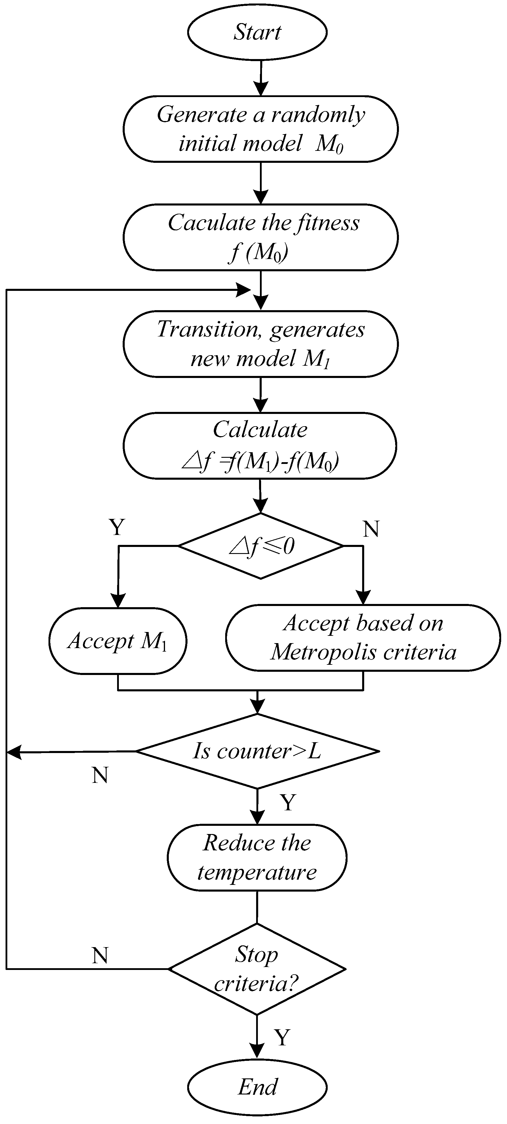
The SAP algorithm is based on the simulation of the solid annealing process. Using the Metropolis acceptance criterion, a set of parameter control algorithm processes, namely the cooling schedule, is established to give the algorithm an approximate optimal solution in polynomial time [46]. The physical image and statistical properties of the solid annealing process are the physical background of the SAP. The Metropolis acceptance criterion guarantees the algorithm will escape the local optimal ‘trap’, and the reasonable choice of the cooling schedule is the prerequisite for the application of the algorithm [47]. The flow chart of the Simulated Annealing Programming Algorithm is shown in Figure 1.
It is calculated by the initial solution and the initial value of the temperature control parameters; the current solution repeats the ‘new solution → calculate the objective function difference → judge whether to accept → accept or discard’ iteration and gradually attenuates the T value. The current solution at the end of the algorithm is the approximate optimal solution. The annealing process is controlled by the cooling schedule parameters, including the initial value of the control parameter and its attenuation factor, the number of iterations per value (called the length of a Markov chain), and the stop condition.
The SAP has the following characteristics [48]: (1) to avoid the loss of the local optimal solution, we accept the worse solution with a certain probability. (2) To improve the reliability of the optimal solution, the SAP algorithm slowly reduces the control parameters, improving the acceptance criterion until the control parameters tend to zero. (3) The objective function requirements are fewer and are not subject to continuous micro-constraints, under which the definition domain can be arbitrarily set. (4) To improve the quality and operation speed of the solution, the introduction of implicit parallelism is employed to solve the nonlinear problem.
2.1.2. Theoretical Model and Variable Selection
The theoretical model to solve the nonlinear model of regional carbon intensity and the key factors is as follows:
where CI is the value of regional carbon intensity, Xit is the t-th year of the i-th key factor, and f(x) is a non-linear function. The key influencing factors are entered into the SAP algorithm in order to find the quantitative relationship between regional carbon intensity and each influencing factor.
Five influencing factors of carbon intensity, including economic development, industrial structure, technological advances, energy price, and social investment, are selected as independent variables for their significance. The mechanism of action is described as follows.
- (1)
- Economic Development. According to Nag and Parikh [49] and Ang [50], there is an inverted U-shaped relationship between economic development and carbon intensity. That is, carbon intensity increases with growing GDP up to a threshold level beyond which carbon intensity drops with higher GDP. The development of the economy not only increases the total amount of carbon emissions, but also improves energy efficiency and reduces carbon intensity levels. Thus, the economy development provides the basic support for the development of technology, laying a strong foundation for the reduction of carbon emission. This study uses per capita GDP indicators to characterize the level of economic development.
- (2)
- Industrial Structure. Yang and Liu [51] believe that the industrial structure is an important factor in differences in carbon emissions levels; Gao [52] believes that the industrial structure, the level of industrialization, and its openness to the public have a significant impact on carbon intensity. This study uses the proportion of tertiary industry to GDP to characterize the impact of industrial structure on carbon intensity.
- (3)
- Technological Advances. It was generally considered that technological advances have a positive effect on CO2 emissions reduction [53,54,55]. The effect is mainly manifested in two ways. First, technological advances can improve the efficiency of mechanical equipment, increase the use of artificial proficiency, and increase output in simple ways, directly reducing carbon intensity. Secondly, technological advances can improve unit energy output, increase the efficiency of the use of social resources, and thereby reduce the social needs of products, product prices, and overall investment, forcing the elimination of excess capacity and the adjustment of the industrial structure, evenly reducing carbon intensity. In this study, total productivity indicators are used to characterize the impact of energy technology.
- (4)
- Energy Price. Greening et al. [56] believed that energy prices had a significant impact on carbon intensity in direct or indirect ways. Chen and Tong [55] argued that the direct impact of energy prices was low. As an indirect impact, energy prices have an effect mainly by adjusting the energy consumption structure, thereby indirectly reducing carbon intensity. As a direct impact, a rise in prices can encourage companies to reduce carbon intensity, reduce their quantity of use, and utilize clean alternative energy sources to improve efficiency. This study uses raw materials, fuel, and the power purchase price index as indicators to characterize energy prices.
- (5)
- Social Investment. Research shows that the expansion of investment levels on carbon emissions has bidirectional effects on carbon intensity [57,58]. On the one hand, the expansion of investment can increase total production scale, thus increasing carbon intensity; on the other hand, the investment increase can drive economic development, which plays a positive role in promoting technological innovation. Former studies show that a modest increase in investment can promote an increase in carbon intensity, but excessive growth is counterproductive. This study uses total societal fixed asset investment as the indicator to characterize the level of social investment.
Five indicators such as per capita GDP, the proportion of tertiary industry to GDP, total productivity, raw materials, fuel, power purchase price index, and total societal fixed asset investment were used to characterize the level of economic development, industrial structure, technological advances, energy price, and social investment respectively.
2.2. Prediction Method of Carbon Emissions Reduction Potential Based on the Genetic Algorithm
A genetic algorithm (GA) is a global optimization search algorithm proposed by a group search strategy and the information exchange between the individuals in the group when the adaptive system is established and gradually developed [59]. Its main characteristic is that it does not depend on gradient information and realizes the evolution of the group by iteration under the premise of using the initial population and genetic operation. The result avoids the local optimum, the search scope is wider, and carbon intensity can be optimized under a multi-target constraint scenario.
According to national economic planning and regional economic and social situations, high growth scenarios, benchmark scenarios (planning scenarios), and low growth scenarios (three economic growth model) all set different policy scenarios, and the global parallel optimization of the GA based on the natural genetic mechanism can be used to optimize carbon intensity under different policy scenarios. The specific calculation process is shown in Figure 2 and described as follows.
- (i)
- Coding. The problem is described as a string through the fitness calculation, wherein each solution corresponds to a fitness value. The project code string is (X1t, X2t, …, Xnt).
- (ii)
- Forming the initial group. The initial population is generated by random method, indicating some things such as a random chromosome, the fixed number of groups, and the project is set to 100.
- (iii)
- Calculating the fitness. The fitness is an indicator of measuring the solution (chromosome) as good or bad and relates to the objective function of the algorithm model. The project fitness calculation function is fitness = f(X1t, X2t, …, Xnt); the corresponding objective function is CIoptimization = Min(fitness).
- (iv)
- Choice. This is the process of entering the next generation directly from the old group, choosing the finest individual.
- (v)
- Cross. This is the process of crossing and converting some parts of chromosomes (strings).
- (vi)
- Mutation. This is to randomly rewrite one or several genes representing a chromosome in a string to represent another trait so that the chromosome is updated.
- (vii)
- Termination. This should repeat (iii), (iv), (v), and (vi). When the optimal population reaches a certain requirement or the evolution of the algebra reaches a set value, it terminates. This study intends to stop when the evolutionary algebra reaches 20 to take the optimal value.
Substituting the key factor control range in different scenarios into the multi-objective optimization program of the above-mentioned GA, we get the CIoptimization and input this value into Equation (1); namely, we obtain the regional carbon emissions reduction potential. In theory, if several factors can be reasonably regulated and balanced, the regional carbon intensity can reach the optimal value (lowest); that is, there is a certain emissions reduction leeway. At the same time, the value of the independent variables corresponding to the optimal carbon intensity represents the policy path that enables the regional carbon emissions reduction potential.
3. Results
As there are both theory and models as discussed above, it is necessary to explore the carbon reduction potential of resource-dependent regions in a typical region with a resource-based economy. Shanxi, a representative resource-dependent province, is chosen for investigation through the SAP model.
3.1. Study Area
Shanxi Province is located in the middle of the Yellow River Basin, which has a population of 36.64 million and covers an area of 156,700 square kilometers. Shanxi is the largest coal production and transportation province as well as an energy and heavy chemical industry base in China. The total area of coal, which accounts for about 40% of the province, is 64,800 square kilometers. Relying on coal resources, the Shanxi economy has achieved rapid development, but, at the same time, it has also created the phenomenon of a ‘coal economy’. The volatility of coal prices has led to swings in regional economies (as shown in Figure 3).
At the same time, even more unsettling is that coal resources have brought about environmental pollution and carbon emissions, which has led to Shanxi Province becoming one of the most carbon-dense regions in China. A development model characterized as long-term and highly dependent on coal resources has raised a series of problems and contradictions by creating regional resource waste, capital outflows, the weakening of institutions, and a decrease in innovation capacity. All of this seriously restricts the development of the local society and economics. Thus, the study of carbon emissions reduction potential in Shanxi Province is a great reference point for the theory and practice of carbon reduction in resource-dependent areas.
3.2. Prediction Model of Carbon Intensity for Shanxi Province
In this section, the prediction model of carbon intensity for Shanxi Province was deduced through the SAP algorithm. The valuable values of the SAP algorithm were determined and the data required were collected. More importantly, a fit test was conducted to verify the validity of the prediction model.
3.2.1. Variable Setting and Data Resources
The carbon intensity in Shanxi Province was selected as the dependent variable, expressed as CI; the influence factors on carbon intensity were selected as the independent variables. X0, the per capita GDP, is an indicator of economic development; X1, the proportion of the tertiary industry in GDP, is an indicator of industrial structure; X2, the total factor productivity, is an indicator of energy technology; X3, the raw material, fuel, and power purchase price index, is an indicator of energy prices; and X4, the total societal investment in fixed assets, is an indicator of social investment. The values of CI and Xi are shown as Table 1.
Considering the availability of data and the difference in the statistical caliber of each year, this study chooses time-series data from 1990 to 2015. The original data of variables in Table 1 were collected from the Shanxi Statistical Yearbook (1991–2016) and the China Energy Statistical Yearbook (1991–2016) and were standardized to eliminate the effect of dimensions. The detailed CI calculation and the carbon emissions coefficients of fossil fuels are provided in Appendix A. The detailed total factor productivity calculations and raw data are provided in Appendix B.
3.2.2. Prediction Model of Carbon Intensity
The data in Table 1 are input into the SAP model given in Section 2.1. The parameters are defined as: initial temperature T0 = 200, termination temperature Tmin = 0, and temperature drop coefficient α = 0.95. The resulting fit coefficient R2 is 0.91, and the fitted equation is given as follows:
3.2.3. Model Fit Test
In this section, goodness of fit tests are performed to verify the superiority of the SAP, and the results are shown in Table 2.
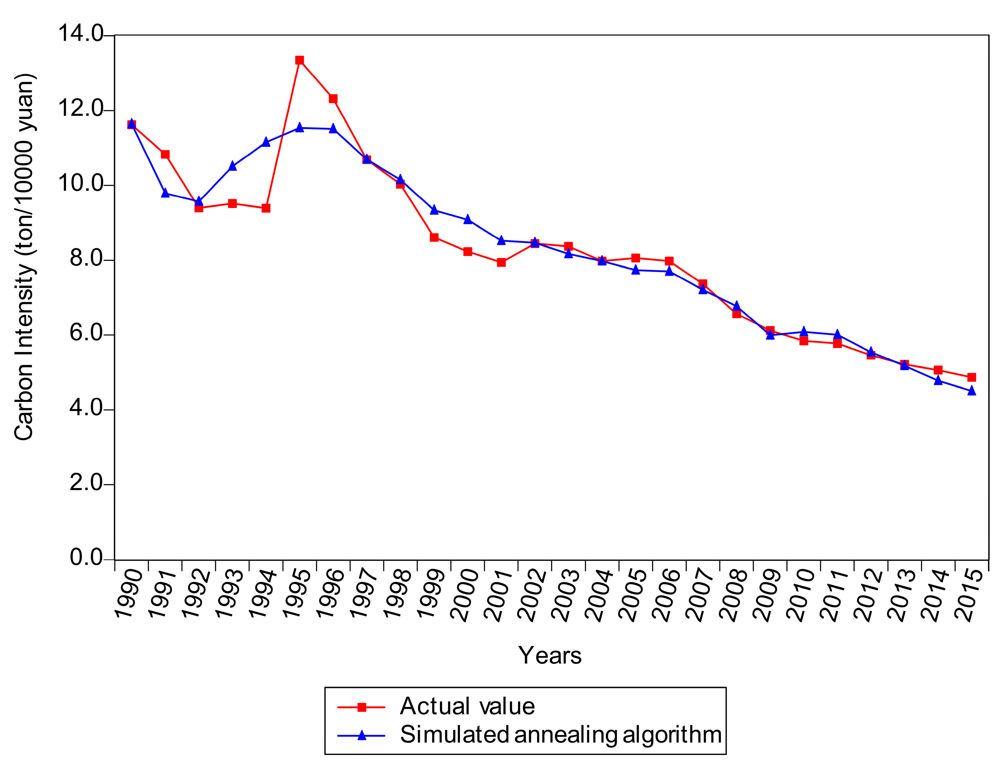
As we can see in Table 2 and Equation (2), the maximum absolute residual of the SAP model is 1.809 in 1995, the minimum absolute residual is 0.002 in 2004, and the fitting degree is 0.91, which is greater than 0.9. Thus, the advantages and feasibility of using the SAP model to construct the prediction model of carbon intensity can be verified. The fitting chart of the carbon intensity prediction model is shown as Figure 4. Obviously, the trend line of the prediction value is similar to that of actual value in Figure 4.
3.3. Analysis on Reachability of Carbon Reduction Targets of 13th Five-Year Work Plan in Shanxi Province
As already stated, according to the ‘13th Five-Year Work Plan for Controlling Greenhouse Gas Emissions’, Shanxi Province has had a target of carbon emissions reduction that translates to a carbon intensity reduction of 18% by 2020. We now estimate whether the carbon emissions reduction target is achievable using the following formula. Q denotes the reachability of the carbon reduction targets of ‘13th Five-Year Work Plan’ in Shanxi Province.
According to the ‘13th Five-Year Work Plan’ of Shanxi Province, the Shanxi Province Development and Reform Commission ‘13th Five-Year Work Plan’ and development program, the Shanxi Province energy development planning, and other ‘13th Five-Year’ control targets, X0 to X4 predictions of Shanxi Province are as follows. X0 = 16,154.7 yuan/person, X1 = 38.25%, X2 = 1.15, X3 = 440.51, X4 = 561.78 billion yuan; input them into Equation (2), the result is 2020 = 3.955 t/10,000 yuan. Table 1 shows the actual carbon intensity in 2015 as 4.87 (t/100,000 yuan); when input it into Equation (3), the result is Q = 18.78%.
As we forecast, the carbon intensity of Shanxi Province in 2020 would be about 18.78% less than that in 2015. This result indicates that the target of carbon reduction, 18% declared in the new five-year (i.e., the ‘13th-Five-Year Work Plan’) will be achieved.
3.4. Estimation of Carbon Emissions Reduction Potential in Shanxi Province during the 13th Five-Year Work Plan
The above assessment shows that the carbon emissions reduction targets in the ‘13th Five-Year Work Plan’ for Shanxi Province can be achieved. However, there appears to be room for additional reduction; we now use the GA to solve this. After taking into account the energy development trend in Shanxi Province, adopting the suggestions of authorities involved and targets set in the ‘13th Five-Year Work Plan’, and holding expert hearings, we reached the expected value of carbon intensity in 2020 in Shanxi Province as follows in Table 3.
After the expected value range of Table 3 is input into the GA optimization program (Figure 1), the results are shown in Table 4.
As can be seen in Table 4, according to the SAP model of 2020, the carbon intensity prediction value is = 3.955 t/10,000 yuan; after further optimization of influencing factors input into the GA program, we find a better carbon intensity value, namely, optimization = 2.985 t/10,000 yuan; this means that for each additional 10,000 yuan of GDP, emissions can be reduced by 0.97 t.
4. Discussion
This study follows the streams of system analysis, system prediction, system optimization and system decision-making. As such it combines the key influencing factors on carbon emissions found in the literature of economic development, industrial structure, energy technology, energy price, and social investment, and then uses a per capita GDP, tertiary industry as a proportion of GDP, total factor productivity, raw materials, fuel, power purchase price index, and total society fixed assets investment as characterization indicators.
- (1)
- The study introduces a SAP algorithm to solve the quantitative relationship between carbon intensity and five influencing factors in Shanxi Province, and establishes a prediction model for carbon intensity. According to the model’s test, the fit degree is strong and the residual values are low. The conclusion is that the SAP algorithm is superior for the prediction of carbon emissions.
- (2)
- According to the model’s forecast, in Shanxi Province, at the end of the ‘13th Five-Year Work plan’, a carbon intensity of 3.955 t/10,000 yuan will be achieved, which is 18.78% lower than the carbon intensity level in 2015; thus, as promulgated by China in its ‘13th Five-Year Work Plan for Controlling Greenhouse Gas Emissions’, the Shanxi Province carbon intensity reduction task of 18% can be achieved.
- (3)
- In Shanxi Province, through the comprehensive evaluation of the policy direction, controlling objectives during the ‘13th Five-Year Work Plan’ and optimizing the influencing factors, the GA can be used to further lower the carbon intensity and thereby further reduce the carbon intensity in Shanxi Province by 0.97 t/10,000 yuan; this means that each additional 10,000 yuan of GDP can achieve a further 0.97 t reduction of emissions in Shanxi Province.
According to the above analysis, we suggest that several measurements are identified in resource-dependent regions to enable carbon reduction potential.
- (1)
- As a big coal region, Shanxi Province has a responsibility to the country; thus, when it implements a carbon emissions reduction policy, several factors should be taken into account, including its actual economic development, population density, and technological advancement, which all contribute to the establishment of a proper low-carbon industrial system. With a low-carbon industrial system, Shanxi not only can solve its outstanding problems, but can also promote equilibrium between coal supply and demand in China, which will promote continuous and scientific development throughout its regional economy, society, and energy and emissions reduction.
- (2)
- In order to provide a big impetus for the province’s coal supply-side structural reform, which will promote its transformation and the upgrade of its economic structure, we should focus on the province’s coal industry by decreasing production capacity, inventories, leverage, and costs, thereby making up for any shortage. In accordance with the law, a number of coalmines have been closed. According to regulations, the reorganization and consolidation of a number of coalmines, reductions, and the withdrawal of the need for excess coal capacity can generate an orderly exit through a market mechanism. In 2016, Shanxi closed 25 coal mines, reducing coal production capacity by 23.25 million tons. By 2020, the province will reduce excess coal capacity by more than 100 million tons.
- (3)
- The coal price formation mechanism needs improvement. A coal price mechanism that can correctly reflect the market supply and demand, the scarcity of resources, and the cost of environmental damage should be explored and established. The role of industry associations should be fostered and a coal pricing self-discipline mechanism should be established. To improve such a price self-discipline mechanism, pilot programs can be established through the Yang Coal Group and the Shanxi Coal Group. In addition, a coal price supervision mechanism could be established and promoted. Further, some reforms can be extended, including reform of the electricity price, the power trading system, the electricity plan, and electricity side sales. To that end, we can cultivate the main electricity sales market, establish and improve the electricity market trading mechanism, and also expand the field and scope of direct supply and raise the electricity market scale in and out of the province. We should also innovate the coal trading mechanism, striving to become a national coal-trading pilot in the near future.
- (4)
- The pace of scientific and technological innovation in the coal industry should be increased. We should establish the Shanxi Coal Clean Utilization Investment Fund. Among other projects, we should focus on supporting coal and electricity integration, the modern coal chemical industry, coal bed methane (gas) extraction and utilization, and carbon trading and carbon emissions reduction. Moreover, to emphasize the clean and efficient use of coal, we should implement a group of major technology innovated coal-based and low-carbon projects. In addition, among other new energy industries, we should foster the development of wind power, photovoltaic power generation, and biomass power generation, which will hasten the development and utilization of new energy industrialization.
- (5)
- In view of our regional economic development characteristics, a flexible carbon emissions reduction mechanism should be built. The Chinese government, over the years, has implemented an extensive administrative control mechanism. Under this system, local government administrations utilize mandatory means to meet the required targets for carbon emissions. As it can directly help these regions to more readily attain these goals, the system is unlike any other, especially in terms of the control of industrial emissions reduction and the elimination of single enterprises. However, among other challenges, the system’s shortcomings lie in issues such as information asymmetry, the high cost of environmental management, the inefficiency of government decision-making, and the inefficiency of government agencies. As for the implementation efficiency and the carbon emissions reduction effect, selecting a reasonable market-based policy tool is still the key to carbon emissions reduction; market-oriented regulatory policies are of two primary types, a price-based carbon tax regime and an aggregate control-based emissions trading scheme. The lack of market-oriented regulation means that enterprises still follow a cost-benefit principle in their investments in carbon emissions reduction, which generates environmental externalities. Compared with the above two policies, the effect of public participation regulation is more lasting, although it is slow. The most important characteristic of the control mechanism is that the driving force is endogenous. If the public’s behavior is insufficient or irresponsible, the mechanism will fail. Only through the comprehensive use of these policies can a flexible mechanism of carbon emissions reduction be established, which will engender greater enthusiasm among the relevant subjects and ensure the realization of carbon emissions reduction targets.
Acknowledgments
We gratefully acknowledge financial support from the National Natural Science Foundation of China, the Investigation on Regulatory Mechanism and Policy of Regional Carbon Emissions Reduction Potential (No. 71373170), the Shanxi Soft Science Project, The mechanism and competency assessment of industrial upgrading driven low carbon transformation in Shanxi province (No. 2017041006), the Shanxi College Students Innovation and Entrepreneurship Training Program, The Innovation Drive Ability and Its Ascension Path of Shanxi Province Based on Low Carbon Development (No. 2017072), the Shanxi Repatriate Study Abroad Foundation (No. 2016-3), and the Program for the Philosophy and Social Sciences Research of Higher Learning Institutions of Shanxi (PSSR) (No. 2015323). The authors would furthermore like to thank the anonymous reviewers and editors for their valuable comments and suggestions on earlier drafts of this paper.
Author Contributions
Wei Li, Guomin Li, and Rongxia Zhang conceived and designed the experiments; Wen Sun performed the experiments; Wen Wu, Baihui Jin, and Pengfei Cui analyzed the data; Guomin Li and Wen Sun contributed reagents, materials, and analysis tools; and Wei Li wrote the paper.
Conflicts of Interest
The authors declare no conflict of interest.
Appendix A
The detailed carbon intensity calculation and the carbon emissions coefficients of fossil fuels are shown as follows.
According to the Shanxi Statistical Yearbook (1991–2016), the China Energy Statistical Yearbook (1991–2016), and the China Entrepreneur Investment Club (CEIC)database, carbon dioxide emissions are calculated using the Standard Coal Coefficient and the Carbon Emissions Coefficients based on the estimation of nine fuel categories (coal, coke, gasoline, crude oil, kerosene, diesel, fuel oil, natural gas, and electricity). At the same time, in order to eliminate the impact of price changes, 1990-based GDP is used; the ratio of the two is the annual value of carbon intensity in Shanxi Province. The formulae are shown as follows:
where i in Formula (A1) is the fossil fuel type (i = 1, …, 9), Ei is the i-th fuel terminal consumption, and CEFi is the carbon emissions coefficient for each of the nine fossil fuels (see Table A1).

Table A1.
The Carbon Emissions Coefficients of fossil fuels.
| Energy Type | Standard Coal Coefficient (kgce/kg) | Carbon Emission Coefficient kg CO2/kgce |
|---|---|---|
| Coal | 0.7143 | 0.7476 |
| Coke | 0.9714 | 0.1128 |
| Gasoline | 1.4714 | 0.5532 |
| Crude oil | 1.4286 | 0.5854 |
| Kerosene | 1.4714 | 0.3416 |
| Diesel | 1.4571 | 0.5913 |
| Fuel oil | 1.4286 | 0.6176 |
| Natural gas | 1.3300 | 0.4479 |
| Electricity | 0.1229 | 2.2132 |
Note: The unit of the Standard Coal Coefficient of natural gas is kgce/m3 (IPCC).
Appendix B
The detailed total factor productivity calculation and raw data are shown as follows.
The DEA method is used to measure total factor productivity. The model used is the traditional Charnes & Cooper & Rhodes (CCR) model and is shown as follows.
where Xij represents the ith input of the jth decision unit and ykj denotes the kth output (ykj > 0) of the jth decision unit. The CCR model can be established by aiming at the efficiency index of the decision-making unit j0 and using the efficiency index of all decision-making units as constraints.
In this study, the output variable is the Total Output Value of State Holding Industrial Enterprises (SHIE) and the inputs are the net value of the fixed assets of SHIE and the mean annual employees of SHIE (see Table A2). Considering the availability of data and the difference in the statistical caliber of each year, this study chooses time-series data from 1990 to 2015; the indicators are from 1990 as the base period was reduced.
Table A2.
The Total Factor Productivity of Shanxi Province from 1990 to 2015.
| Year | Total Factor Productivity | Total Output Value of SHIE (100 Million Yuan) | Net Value of Fixed Assets of SHIE (100 Million Yuan) | Mean Annual Employees of SHIE (10,000 People) |
|---|---|---|---|---|
| 1990 | 0.202 | 95.36 | 568.96 | 168.68 |
| 1991 | 0.200 | 117.73 | 617.48 | 164.36 |
| 1992 | 0.188 | 145.35 | 670.13 | 160.16 |
| 1993 | 0.171 | 179.46 | 727.28 | 156.06 |
| 1994 | 0.176 | 221.56 | 789.30 | 152.06 |
| 1995 | 0.188 | 273.54 | 856.60 | 148.17 |
| 1996 | 0.199 | 337.71 | 929.65 | 144.38 |
| 1997 | 0.221 | 416.94 | 1008.92 | 140.68 |
| 1998 | 0.241 | 514.76 | 1094.95 | 137.08 |
| 1999 | 0.264 | 733.23 | 1186.86 | 133.57 |
| 2000 | 0.283 | 837.80 | 1208.21 | 134.04 |
| 2001 | 0.308 | 954.26 | 1477.74 | 128.42 |
| 2002 | 0.353 | 1075.90 | 1565.59 | 119.90 |
| 2003 | 0.400 | 1375.43 | 1628.87 | 111.47 |
| 2004 | 0.448 | 1950.52 | 1768.87 | 119.04 |
| 2005 | 0.509 | 2534.62 | 2050.57 | 119.84 |
| 2006 | 0.582 | 3048.27 | 2455.02 | 117.98 |
| 2007 | 0.661 | 4038.18 | 2787.29 | 107.79 |
| 2008 | 0.665 | 5199.80 | 3454.90 | 114.56 |
| 2009 | 0.637 | 5188.06 | 3984.60 | 118.35 |
| 2010 | 0.753 | 6614.18 | 4130.20 | 119.16 |
| 2011 | 0.871 | 8207.82 | 5023.63 | 120.47 |
| 2012 | 0.924 | 9620.06 | 5472.79 | 126.48 |
| 2013 | 0.981 | 11,522.96 | 6188.69 | 129.35 |
| 2014 | 0.996 | 13,802.25 | 7155.48 | 132.89 |
| 2015 | 1.000 | 14,257.18 | 7599.46 | 136.32 |
References
- Walther, G.R.; Post, E.; Convey, P.; Menzel, A.; Parmesan, C.; Beebee, T.J.; Fromentin, J.M.; Hoeqh-Guldberq, O.; Bairlein, F. Ecological responses to recent climate change. Nature 2002, 416, 389–395. [Google Scholar] [CrossRef] [PubMed]
- Pan, X.Z.; Teng, F.; Wang, G.H. Sharing emission space at an equitable basis: Allocation scheme based on the equal cumulative emission per capita principle. Appl. Energy 2014, 113, 1810–1818. [Google Scholar] [CrossRef]
- Zhou, P.; Wang, M. Carbon dioxide emissions allocation: A review. Ecol. Econ. 2016, 125, 47–59. [Google Scholar] [CrossRef]
- Matese, A.; Gioli, B.; Vaccari, F.P.; Zaldei, A.; Miglietta, F. Carbon dioxide emissions of the city center of Firenze, Italy: Measurement, evaluation, and source partitioning. J. Appl. Meteorol. Clim. 2009, 48, 1940–1947. [Google Scholar] [CrossRef]
- Kim, B.; Neff, R. Measurement and communication of greenhouse gas emissions from U.S. food consumption via carbon calculators. Ecol. Econ. 2009, 69, 186–196. [Google Scholar] [CrossRef]
- Stremme, W.; Grutter, M.; Rivera, C.; Bezanilla, A.; Garcia, A.R.; Ortega, I.; George, M.; Clerbaux, C.; Coheur, P.F.; Hurtmans, D.; et al. Top-down estimation of carbon monoxide emissions from the Mexico Megacity based on FTIR measurements from ground and space. Atmos. Chem. Phys. 2013, 13, 1357–1376. [Google Scholar] [CrossRef]
- Manafiazar, G.; Zimmerman, S.; Basarab, J.A. Repeatability and variability of short-term spot measurement of methane and carbon dioxide emissions from beef cattle using GreenFeed emissions monitoring system. Can. J. Anim. Sci. 2017, 97, 118–126. [Google Scholar] [CrossRef]
- Zhang, Y.; Zhang, J.Y.; Yang, Z.F.; Li, S.S. Regional differences in the factors that influence China’s energy-related carbon emissions, and potential mitigation strategies. Energy Policy 2011, 39, 7712–7718. [Google Scholar] [CrossRef]
- Tunc, G.I.; Türüt-Aşık, S.; Akbostancı, E. A decomposition analysis of CO2 emissions from energy use: Turkish case. Energy Policy 2009, 37, 4689–4699. [Google Scholar] [CrossRef]
- De Freitas, L.C.; Kaneko, S. Decomposing the decoupling of CO2 emissions and economic growth in Brazil. Ecol. Econ. 2011, 70, 1459–1469. [Google Scholar] [CrossRef]
- Ang, B.W.; Huang, H.C.; Mu, A.R. Properties and linkages of some index decomposition analysis methods. Energy Policy 2009, 37, 4624–4632. [Google Scholar] [CrossRef]
- O’Mahony, T. Decomposition of Ireland’s carbon emissions from 1990 to 2010: An extended Kaya identity. Energy Policy 2013, 59, 573–581. [Google Scholar] [CrossRef]
- Brizga, J.; Feng, K.S.; Hubacek, K. Drivers of CO2 emissions in the former Soviet Union: A country level IPAT analysis from 1990 to 2010. Energy 2013, 59, 743–753. [Google Scholar] [CrossRef]
- Kim, S. LMDI Decomposition Analysis of energy consumption in the Korean manufacturing sector. Sustainability 2017, 9, 202. [Google Scholar] [CrossRef]
- Gutierrez-Velez, V.H.; Pontius, R.G. Influence of carbon mapping and land change modelling on the prediction of carbon emissions from deforestation. Environ. Conserv. 2012, 39, 325–336. [Google Scholar] [CrossRef]
- Asumadu-Sarkodie, S.; Owusu, P.A. Energy use, carbon dioxide emissions, GDP, industrialization, financial development, and population, a causal nexus in Sri Lanka: With a subsequent prediction of energy use using neural network. Energy Sources Part B 2016, 11, 889–899. [Google Scholar] [CrossRef]
- Saleh, C.; Dzakiyullah, N.R.; Nugroho, J.B. Carbon dioxide emission prediction using support vector machine. In Proceedings of the 2nd International Manufacturing Engineering Conference and 3rd Asia-Pacific Conference on Manufacturing Systems, Kuala Lumpur, Malaysia, 12–14 November 2015; Hamedon, Z., Ed.; IOP Conference Series: Materials Science and Engineering: Bristol, UK, 2016. [Google Scholar] [CrossRef]
- Pauzi, H.; Abdullah, L. Prediction on carbon dioxide emissions based on fuzzy rules. In Proceedings of the 3rd International Conference on Mathematical Sciences, Kuala Lumpur, Malaysia, 17–19 December 2013; Zin, W.Z.W., DzulKifli, S.C., Razak, F.A., Ishak, A., Eds.; AIP Publishing: New York, NY, USA, 2014; pp. 222–226. [Google Scholar] [CrossRef]
- Mouazen, A.M.; Palmqvist, M. Development of a framework for the evaluation of the environmental benefits of controlled traffic farming. Sustainability 2015, 7, 8684–8708. [Google Scholar] [CrossRef]
- Solaymani, S.; Yusof, N.; Yavari, A. The role of government climate policy in an oil price shock: A CGE simulation analysis. In Proceedings of the 2015 International Conference on Modeling, Simulation and Applied Mathematics, Phuket, Thailand, 23–24 August 2015; Gholami, M., Jiwari, R., Tavasoli, A., Eds.; MSAM: Phuket, Thailand, 2015; pp. 260–263. [Google Scholar]
- Glotfelty, T.; He, J.; Zhang, Y. Impact of future climate policy scenarios on air quality and aerosol-cloud interactions using an advanced version of CESM/CAM5: Part I. Model evaluation for the current decadal simulations. Atmos. Environ. 2017, 152, 222–239. [Google Scholar] [CrossRef]
- Egbendewe-Mondzozo, A.; Swinton, S.M.; Izaurralde, R.C.; Manowitz, D.H.; Zhang, X.S. Maintaining environmental quality while expanding biomass production: Sub-regional US policy simulations. Energy Policy 2013, 57, 518–531. [Google Scholar] [CrossRef]
- Al-mulali, U.; Sab, C.N.B.C. The impact of energy consumption and CO2 emission on the economic growth and financial development in the Sub Saharan African countries. Energy 2012, 39, 180–186. [Google Scholar] [CrossRef]
- Al-mulali, U. Factors affecting CO2 emission in the Middle East: A panel data analysis. Energy 2012, 44, 564–569. [Google Scholar] [CrossRef]
- Li, H.; Mu, H.; Zhang, M.; Li, N. Analysis on influence factors of China’s CO2 emissions based on Path–STIRPAT model. Energy Policy 2011, 39, 6906–6911. [Google Scholar] [CrossRef]
- Yao, Y.F.; Liang, Q.M.; Yang, D.W.; Liao, H.; Wei, Y.M. How China’s current energy pricing mechanisms will impact its marginal carbon abatement costs? Mitig. Adapt. Strateg. Glob. Chang. 2016, 21, 799–821. [Google Scholar] [CrossRef]
- Wu, F.; Fan, L.W.; Zhou, P.; Zhou, D.Q. Industrial energy efficiency with CO2 emissions in China: A nonparametric analysis. Energy Policy 2012, 49, 164–172. [Google Scholar] [CrossRef]
- Li, H.; Mu, H.; Zhang, M.; Gui, S. Analysis of regional difference on impact factors of China’s energy–Related CO2 emissions. Energy 2012, 39, 319–326. [Google Scholar] [CrossRef]
- Decanio, S.J. The political economy of global carbon emissions reductions. Ecol. Econ. 2009, 68, 915–924. [Google Scholar] [CrossRef]
- Heitmann, N.; Peterson, S. The potential contribution of the shipping sector to an efficient reduction of global carbon dioxide emissions. Environ. Sci. Policy 2014, 42, 56–66. [Google Scholar] [CrossRef]
- Wang, W.; Xie, H.; Jiang, T.; Zhang, D.; Xie, X. Measuring the total-factor carbon emission performance of industrial land use in China based on the global directional distance function and non-radial luenberger productivity index. Sustainability 2016, 8, 336. [Google Scholar] [CrossRef]
- Li, W.; Sun, W. Spatial and temporal distribution characteristics of carbon emission in provincial transportation industry. Syst. Eng. 2016, 11, 30–39. (In Chinese) [Google Scholar]
- Hasegawa, T.; Fujimori, S.; Boer, R.; Immanuel, G.S.; Masui, T. Land-Based mitigation strategies under the mid-term carbon reduction targets in Indonesia. Sustainability 2016, 8, 1283. [Google Scholar] [CrossRef]
- Griffin, P.W.; Hammond, G.P.; Norman, J.B. Industrial energy use and carbon emissions reduction: A UK perspective. WIREE 2016, 5, 684–714. [Google Scholar] [CrossRef]
- Ketelaer, T.; Kaschub, T.; Jochem, P.; Fichtner, W. The potential of carbon dioxide emission reductions in German commercial transport by electric vehicles. Int. J. Environ. Sci. Technol. 2014, 11, 2169–2184. [Google Scholar] [CrossRef]
- Liddle, B. What are the carbon emissions elasticities for income and population? Bridging STIRPAT and EKC via robust heterogeneous panel estimates. Glob. Environ. Chang. 2015, 31, 62–73. [Google Scholar] [CrossRef]
- Wang, F.; Wang, C.J.; Su, Y.; Jin, L.; Wang, Y.; Zhang, X. Decomposition analysis of carbon emission factors from energy consumption in Guangdong province from 1990 to 2014. Sustainability 2017, 9, 274. [Google Scholar] [CrossRef]
- Liang, S.; Zhang, T. What is driving CO2 emissions in a typical manufacturing center of South China? The case of Jiangsu Province. Energy Policy 2011, 39, 7078–7083. [Google Scholar] [CrossRef]
- Wang, Z.; Yang, L. Indirect carbon emissions in household consumption: Evidence from the urban and rural area in China. J. Clean. Prod. 2014, 78, 94–103. [Google Scholar] [CrossRef]
- Zhang, J.; Wang, C.M.; Liu, L.; Guo, H.; Liu, G.D.; Li, Y.W.; Deng, S.H. Investigation of carbon dioxide emission in China by primary component analysis. Sci. Total Environ. 2014, 472, 239–247. [Google Scholar] [CrossRef] [PubMed]
- Dong, X.; Guo, J.; Höök, M.; Pi, G. Sustainability Assessment of the Natural Gas Industry in China Using Principal Component Analysis. Sustainability 2015, 7, 6102–6118. [Google Scholar] [CrossRef]
- Fitzgerald, J.B.; Auerbach, D. The Political Economy of the Water Footprint: A Cross-National Analysis of Ecologically Unequal Exchange. Sustainability 2016, 8, 1263. [Google Scholar] [CrossRef]
- Prakash, S.; Tiwari, M.K.; Lashkari, R.S. A fuzzy goal-programming model of machine-tool selection and operation allocation problem in FMS: A quick converging simulated annealing-based approach. Int. J. Prod. Res. 2006, 44, 43–76. [Google Scholar] [CrossRef]
- Ng, D.; Polito, F.A.; Cervinski, M.A. Optimization of a moving averages program using a simulated annealing algorithm: The goal is to monitor the process not the patients. Clin. Chem. 2016, 62, 1361–1371. [Google Scholar] [CrossRef] [PubMed]
- Suman, B.; Kumar, P. A survey of simulated annealing as a tool for single and multiobjective optimization. J. Oper. Res. Soc. 2006, 57, 1143–1160. [Google Scholar] [CrossRef]
- Kirkpatrick, S.; Gelatt, C.D.; Vecchi, M.P. Optimization by simulated annealing. Science 1983, 220, 671–680. [Google Scholar] [CrossRef] [PubMed]
- Panigrahi, C.K.; Chattopadhyay, P.K.; Chakrabarti, R.N.; Basu, M. Simulated annealing technique for dynamic economic dispatch. Electr. Power Compon. Syst. 2006, 34, 577–586. [Google Scholar] [CrossRef]
- Li, W. Theoretical and Empirical Research on Regional Energy-Saving Potential; Economy & Management Press: Beijing, China, 2012. (In Chinese) [Google Scholar]
- Nag, B.; Parikh, J. Indicators of carbon emission intensity from commercial energy use in India. Energy Econ. 2000, 22, 441–461. [Google Scholar] [CrossRef]
- Ang, B.W. The LMDI approach to decomposition analysis a practical guide. Energy Policy 2005, 33, 867–871. [Google Scholar] [CrossRef]
- Yang, Q.; Liu, H.J. Regional difference decomposition and influence factors of China’s carbon dioxide emissions. J. Quant. Tech. Econ. 2012, 5, 36–49. (In Chinese) [Google Scholar]
- Gao, D.W. Research on Carbon Dioxide Reduction Potential of Central Region and its Influencing Factors. Sci. Technol. Manag. Res. 2014, 2, 49–52. (In Chinese) [Google Scholar]
- Wei, W.X.; Yang, F. Impact of technology advance on carbon dioxide emission in China. Stat. Res. 2010, 7, 36–44. (In Chinese) [Google Scholar]
- Lin, B.Q.; Sun, C.W. How can China achieve its carbon emission reduction target while sustaining economic growth? Soc. Sci. China 2011, 1, 64–76. (In Chinese) [Google Scholar]
- Chen, K.; Tong, X. The Correlation analysis of carbon emissions and its influencing factors in China. Technol. Manag. Res. 2014, 11, 9–12. (In Chinese) [Google Scholar]
- Greening, L.A.; Davis, W.B.; Schipper, L. Decomposition of aggregate carbon intensity for the manufacturing sector: Comparison of declining trends from 10 OECD countries for the period 1971–1991. Energy Econ. 1998, 20, 331–361. [Google Scholar] [CrossRef]
- Lu, Z.N.; Hao, W.L.; Yang, X.L. Factors affecting China’s carbon emissions intensity from low carbon economy perspective. Sci. Technol. Manag. Res. 2016, 3, 240–245. (In Chinese) [Google Scholar]
- Guo, P.; Jiang, G.H.; Zhang, S.X. The Effect of Foreign Direct Investment to China’s Carbon Emissions—An Empirical Study Based on the Provincial Panel Data. J. Cent. Univ. Financ. Econ. 2013, 1, 47–52. (In Chinese) [Google Scholar]
- Chen, G.S.; Chen, X.H. Advances in genetic algorithms. Inf. Control 1994, 23, 215–222. (In Chinese) [Google Scholar]
Figure 1.
The flow chart of the Simulated Annealing Programming Algorithm.

Figure 2.
The flow chart of the Genetic Algorithm.
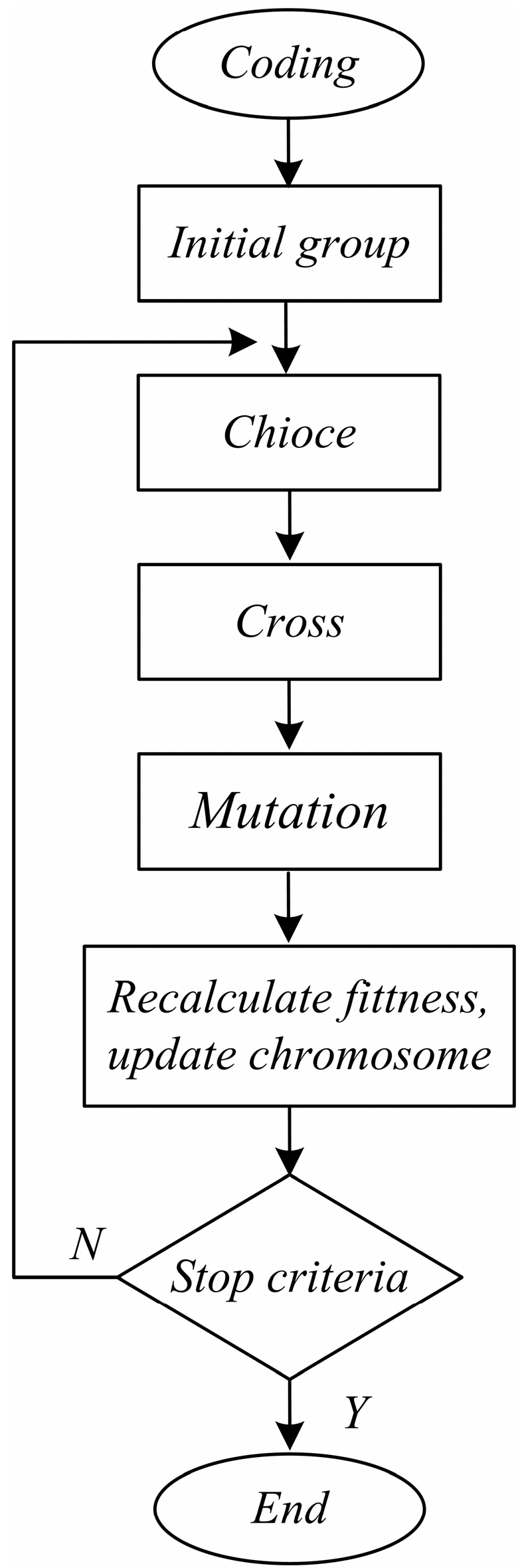
Figure 3.
An overview of economic development in Shanxi Province in China. Note: the data for GDP and industrial value-added are obtained from the Shanxi Statistical Yearbook (1979–2015).
Figure 3.
An overview of economic development in Shanxi Province in China. Note: the data for GDP and industrial value-added are obtained from the Shanxi Statistical Yearbook (1979–2015).
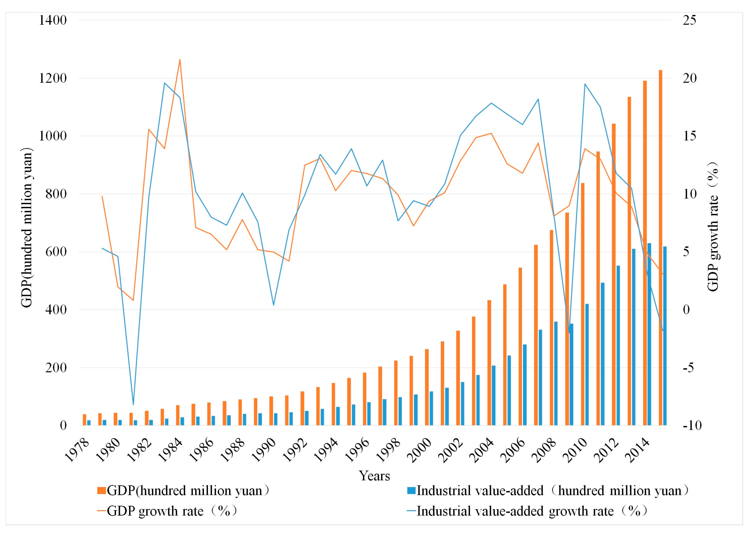
Figure 4.
Fitting chart of the carbon intensity prediction model.

Table 1.
The Carbon Intensity and its influence factors in Shanxi Province from 1990 to 2015.
| Years | CI (t Carbon/10,000 Yuan) | X0 (Yuan/Person) | X1 | X2 | X3 | X4 (10,000 Yuan) |
|---|---|---|---|---|---|---|
| 1990 | 11.62 | 1480.78 | 32.24 | 0.202 | 100.00 | 123.41 |
| 1991 | 10.83 | 1520.40 | 34.31 | 0.200 | 108.01 | 133.04 |
| 1992 | 9.40 | 1689.20 | 34.80 | 0.188 | 120.86 | 155.39 |
| 1993 | 9.51 | 1888.87 | 34.92 | 0.171 | 164.25 | 193.93 |
| 1994 | 9.39 | 2060.50 | 34.89 | 0.176 | 189.06 | 210.02 |
| 1995 | 13.35 | 2284.24 | 35.04 | 0.188 | 213.82 | 224.31 |
| 1996 | 12.32 | 2526.75 | 35.09 | 0.199 | 224.08 | 235.30 |
| 1997 | 10.68 | 2784.72 | 35.76 | 0.221 | 228.57 | 238.83 |
| 1998 | 10.03 | 3030.79 | 35.85 | 0.241 | 222.40 | 235.96 |
| 1999 | 8.61 | 3218.80 | 36.63 | 0.264 | 215.72 | 235.25 |
| 2000 | 8.23 | 3472.89 | 36.83 | 0.283 | 219.82 | 239.49 |
| 2001 | 7.94 | 3796.03 | 37.65 | 0.308 | 223.78 | 243.56 |
| 2002 | 8.44 | 4256.35 | 37.09 | 0.353 | 229.60 | 244.78 |
| 2003 | 8.36 | 4858.86 | 37.30 | 0.400 | 247.51 | 251.87 |
| 2004 | 7.98 | 5564.06 | 37.50 | 0.448 | 283.39 | 264.97 |
| 2005 | 8.06 | 6277.36 | 37.43 | 0.509 | 306.63 | 272.92 |
| 2006 | 7.98 | 7040.28 | 36.50 | 0.582 | 314.61 | 277.01 |
| 2007 | 7.37 | 8116.32 | 36.63 | 0.661 | 331.28 | 288.37 |
| 2008 | 6.56 | 8759.57 | 38.01 | 0.665 | 391.90 | 326.73 |
| 2009 | 6.12 | 9194.59 | 40.11 | 0.637 | 378.58 | 320.52 |
| 2010 | 5.84 | 10,047.33 | 38.61 | 0.753 | 412.65 | 332.38 |
| 2011 | 5.78 | 11,280.38 | 37.29 | 0.871 | 446.08 | 350.66 |
| 2012 | 5.46 | 12,361.70 | 37.32 | 0.924 | 437.60 | 354.87 |
| 2013 | 5.21 | 13,391.54 | 37.02 | 0.981 | 417.91 | 356.64 |
| 2014 | 5.07 | 13,977.79 | 37.80 | 0.996 | 419.33 | 355.21 |
| 2015 | 4.87 | 14,278.4 | 38.78 | 1.000 | 439.47 | 348.82 |
Table 2.
Goodness of Fit tests for the Simulated Annealing Programming model.
| Years | Simulated Annealing Programming Fit Results | Years | Simulated Annealing Programming Fit Results | ||
|---|---|---|---|---|---|
| Fit Value | Residual | Fit Value | Residual | ||
| 1990 | 11.637 | 0.021 | 2003 | 8.169 | −0.196 |
| 1991 | 9.785 | −1.044 | 2004 | 7.978 | 0.002 |
| 1992 | 9.570 | 0.171 | 2005 | 7.740 | −0.319 |
| 1993 | 10.508 | 0.993 | 2006 | 7.706 | −0.273 |
| 1994 | 11.148 | 1.758 | 2007 | 7.210 | −0.158 |
| 1995 | 11.538 | −1.809 | 2008 | 6.769 | 0.207 |
| 1996 | 11.509 | −0.808 | 2009 | 5.997 | −0.119 |
| 1997 | 10.689 | 0.007 | 2010 | 6.083 | 0.241 |
| 1998 | 10.147 | 0.114 | 2011 | 6.007 | 0.230 |
| 1999 | 9.333 | 0.722 | 2012 | 5.545 | 0.082 |
| 2000 | 9.081 | 0.853 | 2013 | 5.177 | −0.035 |
| 2001 | 8.517 | 0.576 | 2014 | 4.785 | −0.281 |
| 2002 | 8.462 | 0.017 | 2015 | 4.509 | −0.361 |
Table 3.
Expected/predicted values of carbon intensity in 2020 in Shanxi Province.
| Type | Predicted Value in 2020 | Expected Value in 2020 | |
|---|---|---|---|
| Variable | |||
| X0 (yuan/person) | 16,154.7 | 14,539.23–17,770.17 | |
| X1 (%) | 38.25 | 31.02–46.54 | |
| X2 | 1.15 | 0.7–1.3 | |
| X3 | 440.51 | 351.58–527.36 | |
| X4 (10,000 yuan) | 561.78 | 279.06–453.47 | |
Table 4.
Comparison of carbon intensity prediction models before and after optimization.
| State | X0 | X1 | X2 | X3 | X4 | |
|---|---|---|---|---|---|---|
| Before | 3.955 | 16,154.7 | 38.25 | 1.15 | 440.51 | 561.78 |
| After | 2.985 | 17,182.56 | 42.66 | 1.28 | 440.66 | 506.29 |
© 2017 by the authors. Licensee MDPI, Basel, Switzerland. This article is an open access article distributed under the terms and conditions of the Creative Commons Attribution (CC BY) license (http://creativecommons.org/licenses/by/4.0/).
Share and Cite
MDPI and ACS Style
Li, W.; Li, G.; Zhang, R.; Sun, W.; Wu, W.; Jin, B.; Cui, P. Carbon Reduction Potential of Resource-Dependent Regions Based on Simulated Annealing Programming Algorithm. Sustainability 2017, 9, 1161. https://doi.org/10.3390/su9071161
AMA Style
Li W, Li G, Zhang R, Sun W, Wu W, Jin B, Cui P. Carbon Reduction Potential of Resource-Dependent Regions Based on Simulated Annealing Programming Algorithm. Sustainability. 2017; 9(7):1161. https://doi.org/10.3390/su9071161
Chicago/Turabian StyleLi, Wei, Guomin Li, Rongxia Zhang, Wen Sun, Wen Wu, Baihui Jin, and Pengfei Cui. 2017. "Carbon Reduction Potential of Resource-Dependent Regions Based on Simulated Annealing Programming Algorithm" Sustainability 9, no. 7: 1161. https://doi.org/10.3390/su9071161
Note that from the first issue of 2016, this journal uses article numbers instead of page numbers. See further details here.