Estimation of the Virtual Water Content of Main Crops on the Korean Peninsula Using Multiple Regional Climate Models and Evapotranspiration Methods

Abstract

Sustainable agriculture in the era of climate change needs to find solutions for the retention and proper utilization of water. This study proposes an ensemble approach for identifying the virtual water content (VWC) of main crops on the Korean Peninsula in past and future climates. Ensemble results with low uncertainty were obtained using three regional climate models, five potential evapotranspiration methods, and the Environmental Policy Integrated Climate (EPIC) crop model. The productivity results of major crops (rice and maize) under climate change are likely to increase more than in the past based on the ensemble results. The ensemble VWC is calculated using three types of crop yields and fifteen consumptive amounts of water use in the past and the future. While the ensemble VWC of rice and maize was 1.18 m³ kg⁻¹ and 0.58 m³ kg⁻¹, respectively, in the past, the future amounts were estimated at 0.76 m³ kg⁻¹ and 0.48 m³ kg⁻¹, respectively. The yields of both crops showed a decline in future projections, indicating that this change could have a positive impact on future water demand. The positive changes in crop productivity and water consumption due to climate change suggest that adaptation to climate change can be an opportunity for enhancing sustainability as well as for minimizing agricultural damage.

1. Introduction

Agriculture is the most climate-dependent production sector; thus, it is necessary to accurately assess the impacts of climate change on the agriculture sector to achieve sustainability [1,2]. The agriculture sector is also linked to the largest number of indicators of sustainable development [3]. The demand for agriculture-related predictions is expected to rise in the future with population expansion and a greater need for food security [4,5].

Agriculture and crop production are the sectors that have the highest water demand [6]. While it is necessary to manage multiple stress factors to achieve agricultural productivity, an abundant supply of water is essential. Several global studies have predicted significant changes in crop productivity and hydrological circulation in the mid-latitude regions during the 21st century [7,8]. The Korean Peninsula has a temperate, monsoon climate with a large annual variation in precipitation, and is classified as a region of water shortage by the UN (United Nations); therefore, it is necessary to study the agricultural water use in the region [9,10].

The concept of virtual water or water footprint has been presented by several international organizations and studies as an effective way to estimate water demand [11,12]. Virtual water refers to the amount of water used per unit product and is synonymous with water footprint. Many studies have estimated the water demand of the agricultural sector by calculating the virtual water of crops [13,14,15]. By estimating the virtual water per crop, we can also analyze the influence of regional differences and climate change on the water demand.

While estimates of the virtual water content of crops in East Asian cases can be easily found [11,12,13,14,15,16], the crop-hydrological model-based estimation approach for production and water consumption is not common. In particular, there were no cases which estimated the virtual water of a crop with a model-based approach on the Korean Peninsula, and only Zhao et al. [15] suggested the virtual water of several crops in China using a modeling approach. The information from a model-based virtual water content analysis in the Korean Peninsula can help solve problems of food and water security [4,10].

Previous model-based virtual water studies have calculated the amount of water used, crop yields, and evapotranspiration rates to estimate the virtual water content of crops [13,15,16]. The most basic data used in the estimation of evapotranspiration and crop yield is climatic data, which has significant uncertainties [10,17], depending on the climate model used [9,18].

To estimate and reduce uncertainties in a model’s predictions, multiple methods have recently been employed by the crop modeling community [17,19,20,21]. The major source of a model’s error is from the uncertainty of the input data, such as climate data. Another source is due to a model’s characteristics having various approaches and parameterizations to determine the growth and the phenological development of the crop [20].

In this study, we propose a multi-input and multi-model super ensemble approach for the virtual water content of main crops based on the past and future climate data of the Korean Peninsula. Specifically, we use five evapotranspiration methods to reduce model uncertainty and three regional climate models to reduce the uncertainty in the climate data. In particular, we present virtual water content that represents the past and the future by averaging the number of virtual water contents based on multiple data and methodologies. The average of the multiple results is defined as the ensemble average, and the uncertainty reduction is analyzed by considering the difference in each value without considering the variability. Given the importance and increasing emphasis of agricultural water use under climate change, it is useful to provide the estimation of the ensemble virtual water of main crops.

2. Data and Methods

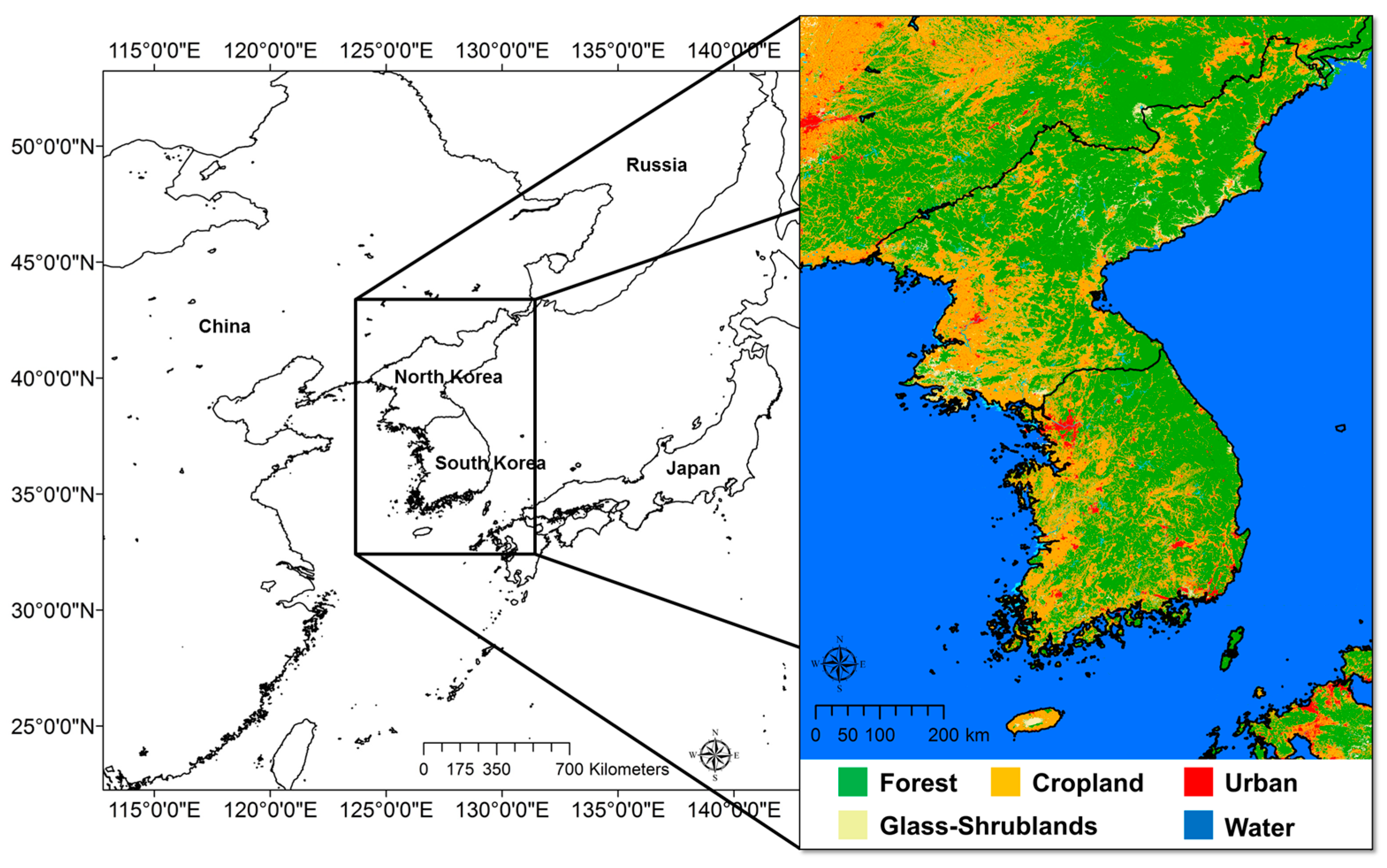
2.1. Research Area and Crops

The research area covers the whole cropland of the Korean Peninsula, which includes both South and North Korea (Figure 1). The Korean Peninsula is located on the eastern end of Asia, covers an area of about 221,000 km², and is located between the 33.23° N and 43.01° N latitudes and the 124.14° E and 130.93° E longitudes. The Korean Peninsula is located in the temperate zone. It is largely influenced by the temperate monsoon climate, and has large annual variations in precipitation, with high temperatures and humidity levels in the summer. Under the Köppen climate classification, a warm and dry winter climate (Cwa) and a cold and dry winter climate (Dwa) are the most common, with an average annual temperature of 10–16 °C, and an average cumulative precipitation of 1200 mm [22]. Geographically, there are high mountains in the north and east and plains in the south and west.

The cropped area of South Korea is about 20,000 km² and that of North Korea about 30,000 km², which is over 20% of the total area of the peninsula. Rice paddies and maize fields appear to be mixed, but rice is widely distributed on a broad plain and the number of maize fields increases in the north [23]. In this study, considering the resolution of the available climate data, the cropland of the peninsula was mapped with a 5 km² grid resolution, and all the data were processed accordingly.

In this study, rice and maize, staple crops in the Korean Peninsula, are selected for the analysis. Rice production is dominant throughout the region, where precipitation is concentrated in the summer. Maize is mainly produced in the northeastern region, where low precipitation and temperature conditions are dominant. Note that maize accounts for 35% of the total food production in North Korea [23,24].

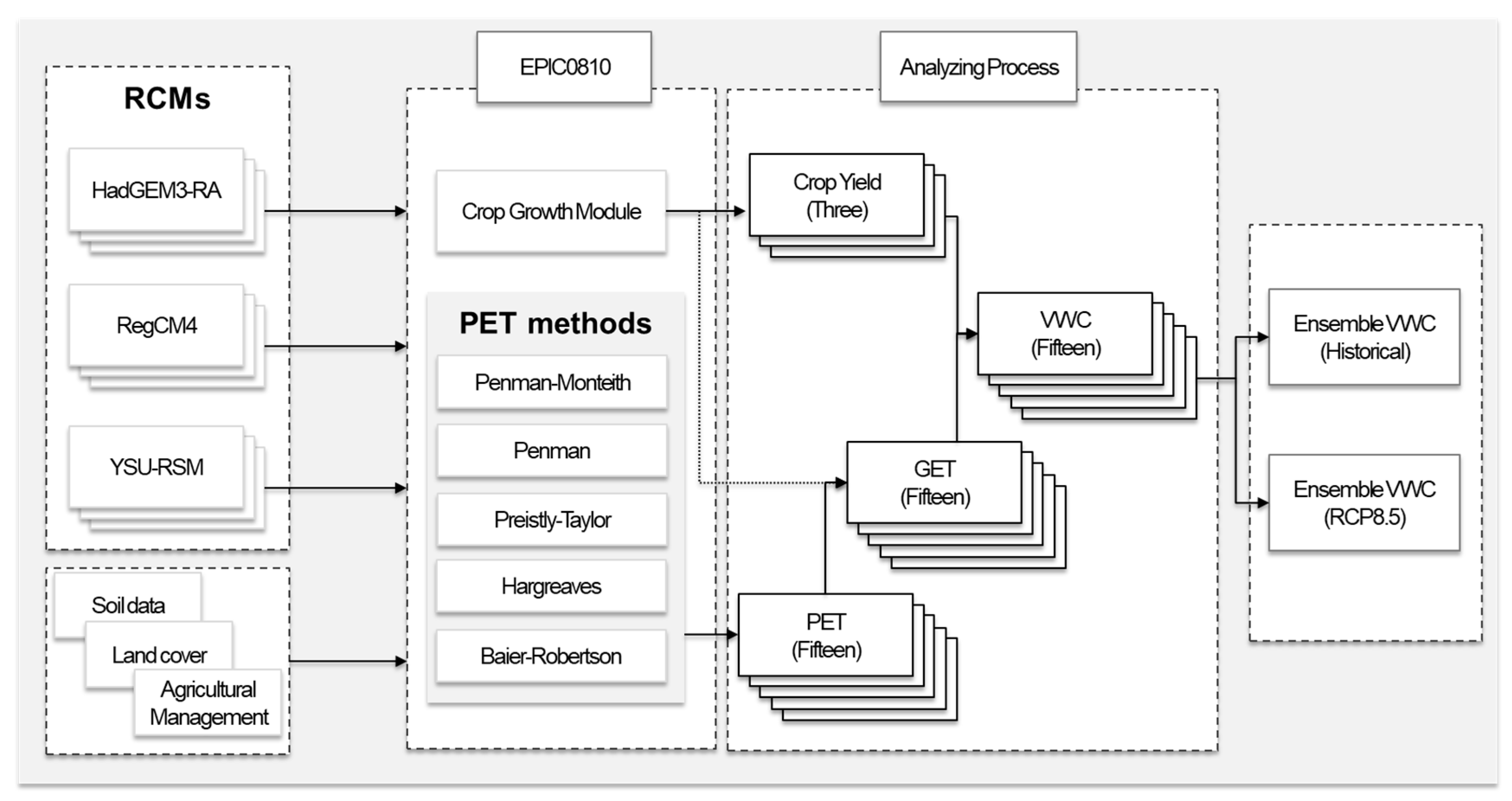
2.2. Assessment Model Hierarchy

Figure 2 shows a data flow of this study. We have selected three regional climate models (RCM) for climate data, and each climate data are used in a simulation in an EPIC model with five different potential evapotranspiration (PET) methods. In the research framework, fifteen ensemble members are produced and are used to estimate the virtual water contents (VWC) of crops over the study region. A detailed explanation of each component is described in the following sections.

2.3. Multiple Regional Climate Models

To reduce the uncertainty in the climate data, the data of three regional climate models (RCM) were used. The climate model data for the region are obtained through the COordinated Regional climate Downscaling EXperiment (CORDEX)-East Asia. The CORDEX initiative was launched by the Task Force for Regional Climate Downscaling (TFRCD), which was established in 2009 by the World Climate Research Program (WCRP).

The climate data of the RCMs acquired through CORDEX-East Asia are HadGEM3-RA, RegCM4, and YSU-RCM, and the three models were verified using previous studies [10,17]. These models provide dynamically downscaled data with a spatial resolution of 12.5 km² based on the HadGEM2-AO model, a large-scale climate model.

HadGEM3-RA is a regional version of the Hadley Center Global Environment Model, a non-hydrostatic regional climate model following the Arakawa-C horizontal grid and a terrain-following vertical coordinate [9]. RegCM4, the fourth version of the RegCM regional climate model system, is a hydrostatic, compressible model with sigma-p vertical coordinates and an Arakawa-B horizontal grid [25]. YSU-RSM, a disturbance model, is defined by a two-dimensional sine series for the perturbation of vorticity and by a two-dimensional cosine series for perturbations of pressure, divergence, temperature, and mixing ratio [26]. More detailed information about these models can be found on the CORDEX-East Asia web page (https://cordex-ea.climate.go.kr/main/aboutCordexPage.do).

We used RCMs for the representative concentration pathways (RCP) 8.5 scenario, which is the lowest greenhouse gas reduction scenario, and for the analysis of the data for 1981–2000 and 2031–2050.

2.4. EPIC Model and PET Methods

The EPIC model was developed in the 1980s to assess soil erosion and soil productivity, followed by a model on plant growth and hydrological parameters [27,28]. Since the EPIC model was first published, many components have been added, such as GLEAMS [29], Century [30], and RUSLE [31]. This model was renamed the Environmental Policy Integrated Climate model (EPIC) with the addition of environmental assessment functions for pesticides and water quality [32].

The EPIC model has a structure that converts daily energy and biomass to simulate crop growth [28]. The daily potential biomass increase is calculated using climate variables such as the solar radiation and biomass–energy conversion rates of the crop. The daily response to plant stress variables (water, nutrient, temperature, aeration, and salinity) decreases the potential biomass. Crop yields are ultimately estimated based on the crop harvest index and the actual biomass accumulation [33].

The estimation of crop productivity through the EPIC model has been successfully applied to the whole of the Korean Peninsula, as well as Eastern Asia, by previous studies [34,35,36]. In this study, calibration was performed to estimate the crop productivity on the Korean Peninsula. Some of the key crop parameters were modified through calibration. For rice, the biomass–energy ratio was set at 30 kg MJ⁻¹, the harvest index at 0.55 mg mg⁻¹, the optimum temperature at 25 °C, the base temperature at 10 °C, and the potential heat unit (PHU) ranged from 1300 to 1500 °C, depending on the climate of the specific grid cells. For maize, the biomass–energy ratio was set at 43 kg MJ⁻¹, the harvest index at 0.45 mg mg⁻¹, the optimum temperature at 25 °C, the base temperature at 8 °C, and the PHU range at 1000–1200 °C, depending on the climate of the specific grid cells [34,37,38].

After calibration, a statistical validation was conducted to evaluate the model’s performance for estimating crop productivity using the results from 1981 to 2000 and the statistical data. The HadGEM3-RA climate model was used as a standard in the calibration and validation process. HadGEM3-RA has been used most commonly for the Korean Peninsula and shown to average between the RegCM4 and YSU-RSM [17,18,39]. Since only the amount of production by country is known and the statistics for North Korea are very limited, the model was only verified for the South Korean data. The statistical data on rice and maize production were retrieved from the Korea Statistical Information System (KOSIS). Three statistical indicators were used to validate the model’s performance: (i) the Root Mean Square Error (RMSE), (ii) the Nash–Sutcliffe Efficiency Coefficient (NSEC), and (iii) the Relative Error (RE) [40,41]. These statistical measures have been described in detail in the literature [35,37,42].

Five representative methods (Penman–Monteith (PM) [43], Penman (P) [44], Preistly–Taylor (PT) [45], Hargreaves (H) [46], and Baier–Robertson (BR) [47]) were used to estimate the PET. All of the PET methods available in the EPIC model were used, and these five methods are commonly used in equations in many previous studies [12,13,14,15,21].

$${\mathrm{PET}}_{\mathrm{PM}}=\left(\mathrm{RN}\times \mathsf{\delta }+86.66\times \mathrm{AD}\times \mathrm{EA}\left(1-\mathrm{RH}\right)\times \mathrm{U}/350\right)/\left(\left(2.51-0.0022\times \mathrm{T}\right)\times \left(\mathsf{\delta }+\mathsf{\gamma }\right)\right)$$

(1)

$${\mathrm{PET}}_{\mathrm{P}}=\left(\mathrm{RN}\times \mathsf{\delta }/(2.051-0.0022\times \mathrm{T})+\mathsf{\gamma }\times \left(2.7+1.63\times \mathrm{U}\right)\times \mathrm{EA}\left(1-\mathrm{RH}\right)\right)/\left(\mathsf{\delta }+\mathsf{\gamma }\right)$$

(2)

$${\mathrm{PET}}_{\mathrm{PT}}=1.28\times \left(\mathrm{RN}\times \left(1.0-\mathrm{AB}\right)/\left(2.501-0.0022\times \mathrm{T}\right)\right)\times \left(\mathsf{\delta }/\left(\mathsf{\delta }+\mathsf{\gamma }\right)\right)$$

(3)

$${\mathrm{PET}}_{\mathrm{H}}=0.0032\times \left(\mathrm{RAMX}/\left(2.501-0.0022\times \mathrm{T}\right)\right)\times \left(\mathrm{T}+17.8\right)\times {\left({\mathrm{T}}_{\max }-{\mathrm{T}}_{\min }\right)}^{0.6}$$

(4)

$${\mathrm{PET}}_{\mathrm{BR}}=0.288\times {\mathrm{T}}_{\max }-0.144\times {\mathrm{T}}_{\min }+0.139\times \mathrm{RAMX}-4.931$$

(5)

PET_PM, PET_P, PET_PT, PET_H, and PET_BR simulate the daily PET by each method. T_min and T_max are the daily minimum and maximum temperatures (°C), and RAMX is the solar irradiance on a clear day (MJ m⁻² d⁻¹). T is the slope of the daily average temperature (°C), RN is the total solar irradiance (MJ m⁻² d⁻¹), δ is the slope of the saturation vapor pressure curve (kPa °C⁻¹), γ is the psychrometric constant (kPa °C⁻¹), U is the average daily wind speed (ms⁻¹), and EA is the saturation vapor pressure at mean air temperature (kPa). RH is the average relative humidity per day, AD is air density (Kg m⁻³), and AB is the soil albedo. The required meteorological data are different for each PET method. PET_PM and PET_P require the temperature, solar radiation, relative humidity, and wind speed variables; PET_PT requires the relative humidity and wind speed values; and PET_H and PET_BR require only the temperature-related variables. The climate requirement of each PET method is described in

Table 1. Climate variables required by each PET method (○: Required climate variables).

Method	Temperature (T, Tmin, Tmax)	Solar Radiation	Relative Humidity	Wind Speed	Reference
Penman–Monteith	○	○	○	○	Monteith (1965)
Penman	○	○	○	○	Penman (1948)
Priestley–Taylor	○	○			Priestley and Taylor (1972)
Hargreaves	○				Hargreaves and Samani (1985)
Baier–Robertson	○				Baier and Robertson (1965)

.

2.5. Method to Calculate Virtual Water Content of Crops

The method proposed by Zhao et al. [15] to estimate the virtual water content (VWC) of crops was used in this study. The VWC of crops represents the amount of water used per unit of production, defined as the ratio of the Consumptive Water Use (CWU) to crop production [48]. The CWU of the crop is estimated from the actual evapotranspiration during the growing season of each crop. The VWC of the crop is an indicator of the agricultural demand, which can be used to estimate the total demand for water in the region and the supply requirements. The VWC is calculated as follows.

$$\mathrm{VWC}=\mathrm{CWU}/\mathrm{P}=10\times \mathrm{GET}/\mathrm{Y}$$

(6)

where CWU is the volume of water (m³) used by the crop during the growing season, P is the amount of crop (kg) produced during the same period, GET is the actual evapotranspiration in the growing season (mm), Y is the crop yield in kg ha⁻¹ units, and the number 10 was used for the conversion of mm to m³ ha⁻¹.

2.6. Other Data and Management Description

The EPIC model requires various soil-related parameters (OC (%), pH, cation exchange capacity (cmol kg⁻¹), sand (%), silt (%), bulk density (tm⁻³), and electrical conductivity (mS cm⁻¹)). The input form was completed using the Digital Soil Map of the World [49], constructed spatially using the ISRIC-WISE database [50].

We used the 2010 Global Land Cover 30 (GLC30) data to reflect the current land cover [51] (accessed from http://www.globallandcover.com). GLC30, a 30 m land cover map based on Landsat 7 satellite imagery, was extracted from the cropland of the Korean peninsula and constructed with 5 km × 5 km grid cells.

The amount of fertilizer and irrigation water required for each crop and area in the EPIC model is calculated to determine the spatially required amount. Since the planting and harvest dates for crops are different for each region, these are automatically assigned based on the temperature by setting the first farming start date to reflect agricultural activities on the Korean Peninsula. The starting date of the first farming for rice was set to 1 March and for corn, to 1 April.

3. Results

3.1. Estimation of Crop Yield

3.1.1. Evaluation of the Model’s Performance

The HadGEM-EPIC results were used for evaluating the model’s performance (

Table 2. Evaluation of the model’s performance in estimating rice and maize yield. SD, standard deviation; RMSE, root mean square error, NSEC, Nash–Sutcliffe efficiency coefficient; RE, relative error.

Year	Reported (t ha−1)		Estimated (t ha−1)		RMSE	E (NSEC)	RE (%)
	Mean	SD	Mean	SD
Rice Yield
1981	4.03	0.39	3.96	0.36	0.28	−0.41	−1.12
1982	4.21	0.38	5.16	0.33	0.59	−0.71	3.35
1983	4.20	0.39	5.12	0.37	0.51	−1.01	4.28
1984	4.38	0.40	4.77	0.54	0.40	−0.01	1.79
1985	4.31	0.42	4.81	0.45	0.57	−0.65	5.21
1986	4.25	0.68	4.85	0.43	0.63	−0.72	2.56
1987	4.19	0.42	4.08	0.27	0.31	−0.08	−1.93
1988	4.64	0.45	4.98	0.31	0.44	−0.48	1.52
1989	4.56	0.34	4.67	0.41	0.32	−0.09	0.69
1990	4.34	0.42	4.87	0.56	0.56	−1.08	2.87
1991	4.28	0.34	4.69	0.27	0.48	−0.57	1.36
1992	4.44	0.34	5.44	0.63	0.87	−0.82	3.82
1993	4.08	0.58	4.84	0.33	0.74	−1.16	2.61
1994	4.45	0.32	4.56	0.45	0.27	−0.25	0.42
1995	4.35	0.28	4.90	0.29	0.59	−0.89	1.93
1996	4.94	0.26	4.56	0.36	0.41	−0.12	−1.25
1997	5.00	0.32	4.89	0.42	0.37	−0.08	−0.73
1998	4.62	0.36	5.01	0.43	0.45	−0.33	1.13
1999	4.78	0.37	3.91	0.27	0.77	−1.02	−3.27
2000	4.80	0.31	4.99	0.44	0.29	−0.04	1.11
Maize Yield
1981	4.38	1.58	4.32	0.18	0.42	−0.51	−0.81
1982	4.12	1.37	5.20	0.38	0.87	−1.12	3.67
1983	3.66	1.24	5.36	0.28	1.21	−2.33	6.15
1984	4.44	1.61	5.05	0.33	0.75	−0.62	2.49
1985	5.04	1.76	5.26	0.33	0.38	−0.09	1.22
1986	4.79	1.71	5.47	0.43	0.73	−0.43	5.76
1987	4.85	1.63	4.60	0.29	0.42	−0.11	−1.93
1988	4.80	1.93	5.25	0.25	0.55	−0.91	7.32
1989	4.88	1.84	4.38	0.22	0.65	−1.15	−1.86
1990	4.61	1.78	5.07	0.29	0.71	−1.32	2.83
1991	3.41	1.34	5.57	0.37	1.63	−2.78	12.32
1992	4.40	1.52	5.63	0.38	0.88	−1.18	8.17
1993	4.18	1.54	5.15	0.29	0.91	−1.36	5.86
1994	4.09	1.53	4.39	0.27	0.37	−0.12	1.04
1995	4.25	1.54	5.19	0.35	0.82	−0.58	3.63
1996	4.03	1.60	5.83	0.29	1.44	−2.30	8.29
1997	4.11	1.48	5.19	0.27	1.01	−0.91	5.59
1998	3.98	1.31	4.68	0.30	0.71	−1.21	5.15
1999	3.94	1.37	5.30	0.30	1.09	−0.81	10.28
2000	4.06	1.16	5.06	0.24	0.91	−1.11	9.11

). The statistical data for the rice yield showed an average range of 4.0–5.0 t ha⁻¹ with a low standard deviation. The maize yield data showed relatively high standard deviations and an average of 3.6–5.1 t ha⁻¹. The non-main production area for maize had a very low yield, which led to high standard deviations. The estimates showed low standard deviations and were similar to the reported values. The RMSE values ranged from 0.2 to 0.9 for rice and 0.3 to 1.7 for maize, rice data showing higher accuracy (Table 2). The NSEC and RE values showed that the rice yield data were more accurate, which contributed to the high standard deviations of the maize production data (Table 2). The accuracy assessment of the statistical data for the two crops showed an overall high degree of accuracy; therefore, the data can be used in past climate models and in future climate change research.

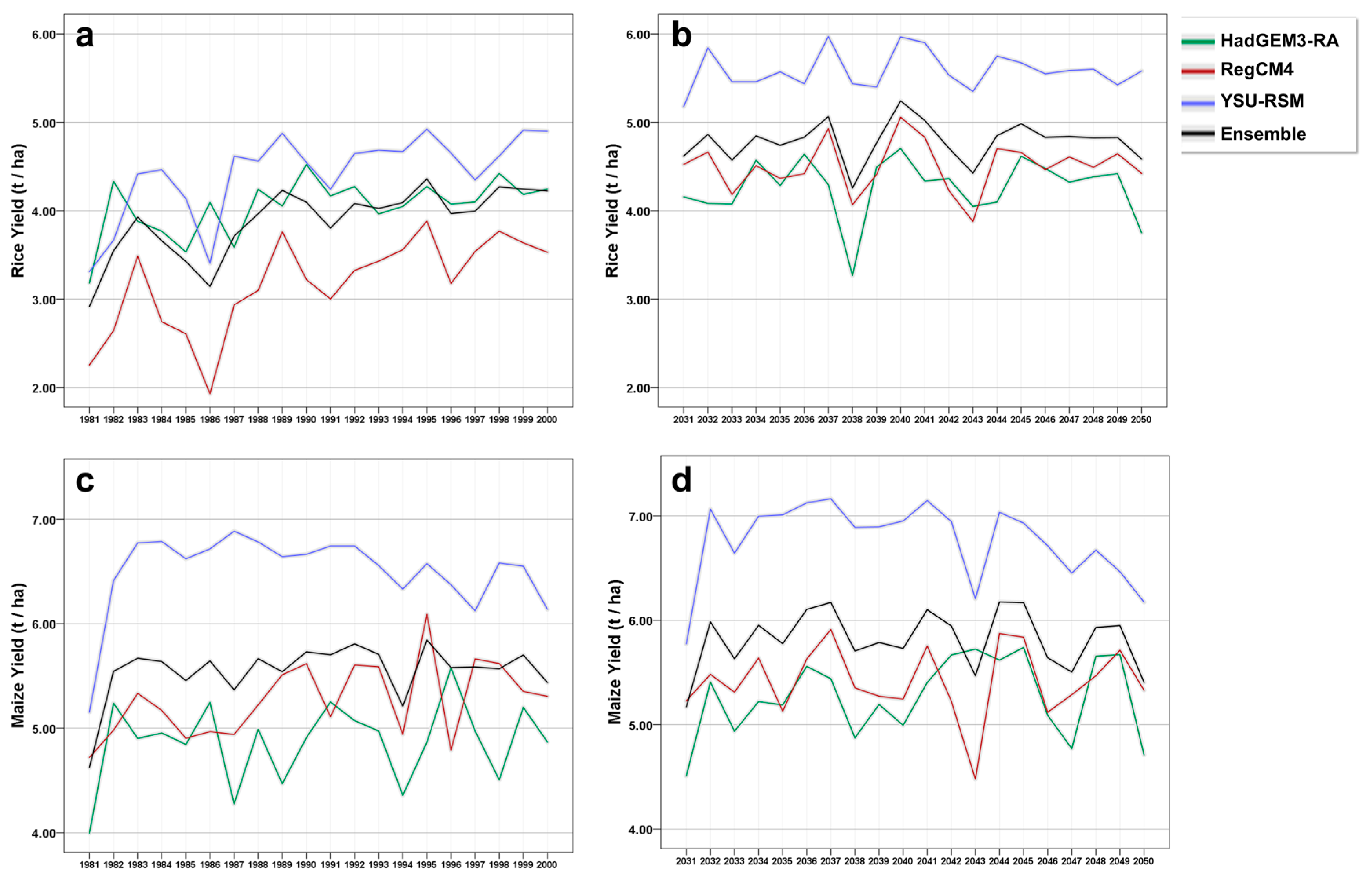
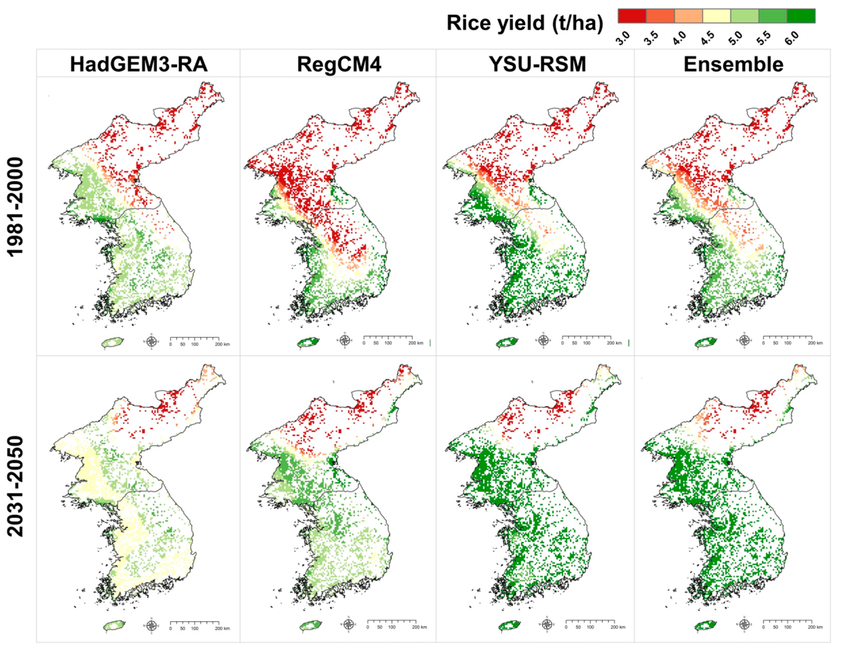
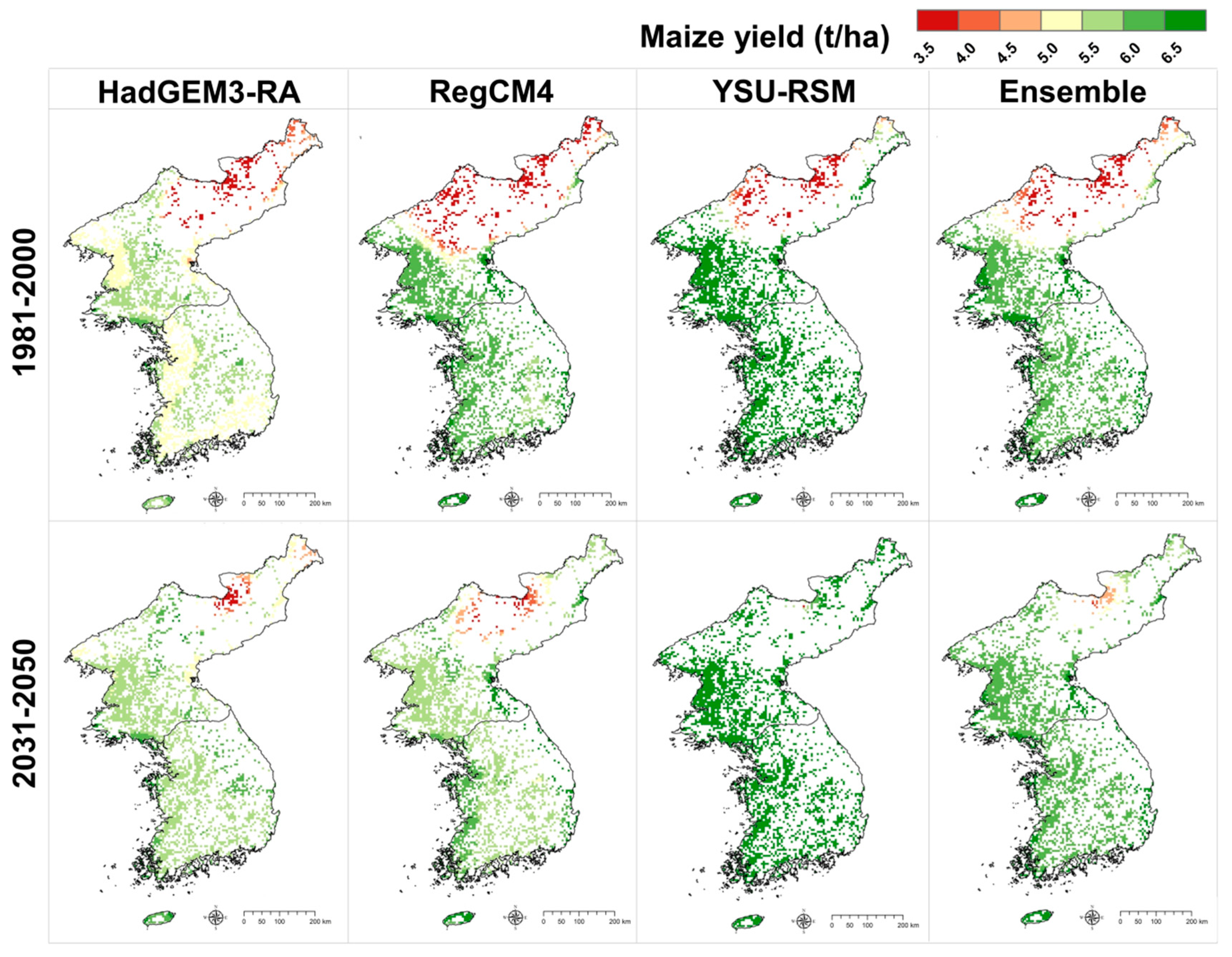
3.1.2. Estimation of Crop Yields Using Multiple RCMs

The estimated results of rice and maize production using three RCMs showed significant differences between the models. Based on the RCP 8.5 scenario, the productivity is predicted to increase in the future.

Rice yields showed a gradual increase from 1981 to 2000, and the RegCM4-EPIC result was the lowest (mean 3.1 t ha⁻¹) while the YSU-RSM-EPIC result was the highest (mean 4.25 t ha⁻¹) (Figure 2). The estimation results of HadGEM3-RA-EPIC were moderate (mean 4.05 t ha⁻¹), and the values of the three ensembles (mean 4.25 t ha⁻¹) were similar to those of HadGEM3-RA-EPIC (Figure 2). The results of the ensemble were similar to the agricultural statistics, and more accurate than the individual model results (Figure 2 and Table 2). The spatial distribution of productivity calculated by RegCM4-EPIC showed that the whole of North Korea and the central region of South Korea had low productivity. YSU-RSM-EPIC showed high productivity in the entirety of South Korea, while HadGEM3-RA-EPIC showed high productivity in the western plains of North Korea (Figure 3). The rice cultivation on the Korean Peninsula was more accurately expressed in the ensemble results than the individual model results, compared to the existing studies or the actual production status [52,53].

In the RCP 8.5 scenario for 2031–2050, the rice productivity estimates are predicted to increase by 15–25% compared to the historical data. In the historical data, the YSU-RSM-EPIC results were the highest (mean 5.6 t ha⁻¹), while the RegCM4-EPIC results were slightly higher than the HadGEM3-RA-EPIC results. The ensemble results showed an average rice yield of 4.7 t ha⁻¹, with annual variability, but not with a time series increase or decrease (Figure 3). Differences in spatial distribution between the models were observed, but overall, rice productivity improved in most regions except the northeast mountainous region of the Korean Peninsula (Figure 4).

The maize yield results showed no significant increase or decrease from 1981 to 2000, but the YSU-RSM-EPIC results (mean 6.4 t h⁻¹) were the highest, similar to those for the rice data. RegCM4-EPIC showed moderate levels (mean 5.25 t ha⁻¹), while the lowest results were calculated by HadGEM3-RA-EPIC (mean 4.85 t ha⁻¹). The ensemble results showed an average value of 5.5 t ha⁻¹ (Figure 3), which was similar to the existing Korean Peninsula maize productivity data [34]. Most regions, except the high plateau region of the Korean Peninsula, showed high productivity, which was more evident in the ensemble results (Figure 5).

The estimates of the future maize productivity, from 2031 to 2050, under climate change showed a slight increase in productivity compared to past productivity. The YSU-RSM-EPIC results were the highest, and the RegCM4-EPIC results were slightly higher than the HadGEM3-RA-EPIC results (Figure 3). The ensemble results showed an average maize yield of 5.75 t ha⁻¹, with annual variability, but no significant increase in the time series. There was no significant difference in spatial distribution between the models, and maize productivity was found to increase across the Korean Peninsula (Figure 5).

Three RCM and EPIC models were used to estimate the change in crop productivity, which was then used as an ensemble result to reduce the uncertainty in the climate models. This ensemble result considers the fertilization and irrigation required for crop growth, and is estimated for the whole cultivation area without distinguishing between rice paddies and maize fields.

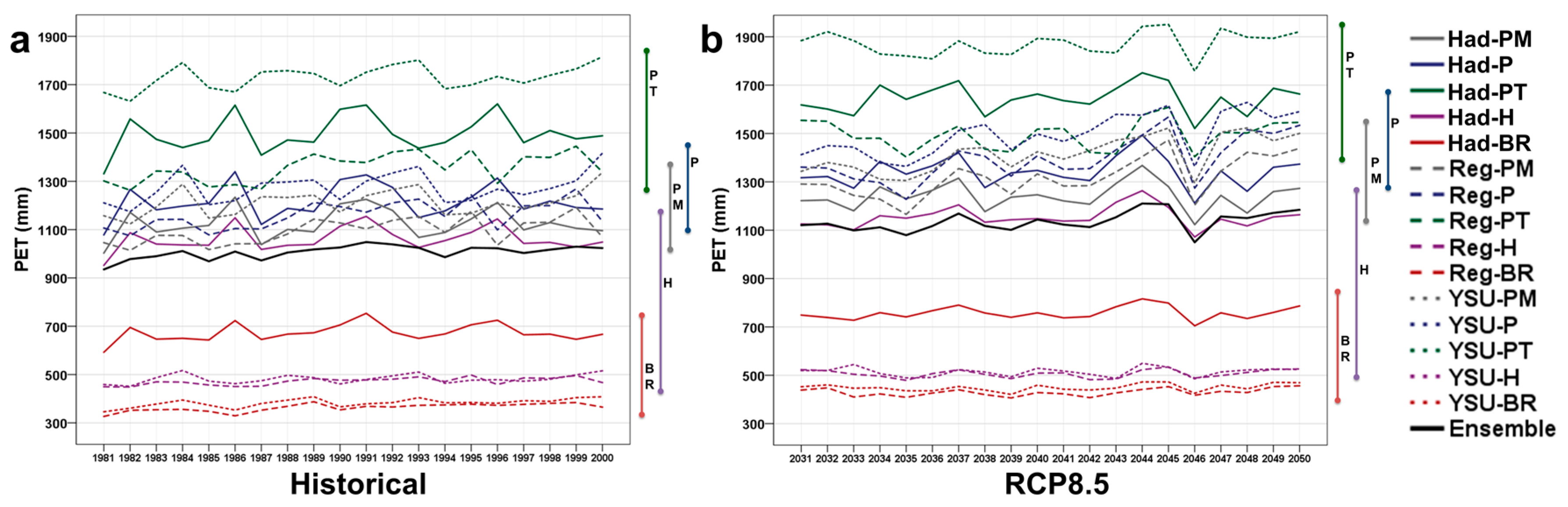
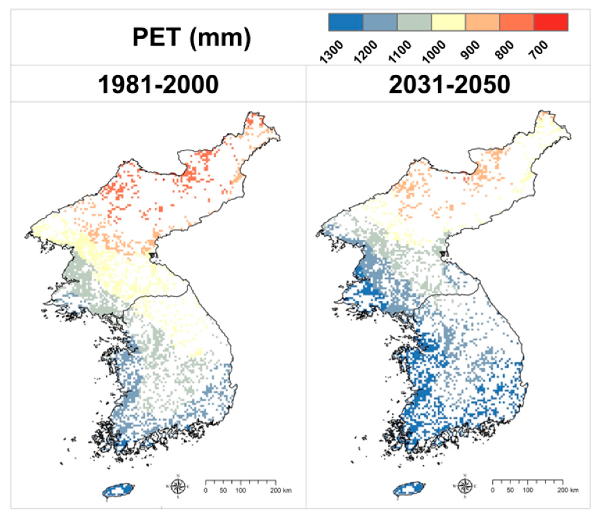
3.2. Estimation of PET Using Multiple Methods

Three RCMs and five PET methods were used to estimate a total of fifteen PETs in the Korean Peninsula. The PET estimation results were greater than the RCM results by over 1000 mm per year. The annual variations were minimal, and the differences between the RCM or PET method results were greater. Although all five methods were representative PET methods, the PET was largely overestimated and the BR was largely underestimated. The trends in the results for each past and future model (RCP 8.5) were similar, but the values were predicted to increase by 100 mm in the future (Figure 6). The ensemble values of the fifteen results confirmed that latitudinal differences were prevalent. In the past ensemble results, South Korea showed a PET level of 1000–1300 mm and North Korea 700–1100 mm. In the future, the PET levels for both South and North Korea are predicted to increase by an average of 100 mm (Figure 7).

The ensemble values were similar to the results of the existing PET studies in the Korean Peninsula or the satellite-based estimates when compared to the fifteen individual results, and the ensemble results for the future analysis period had a low level of uncertainty [41,54].

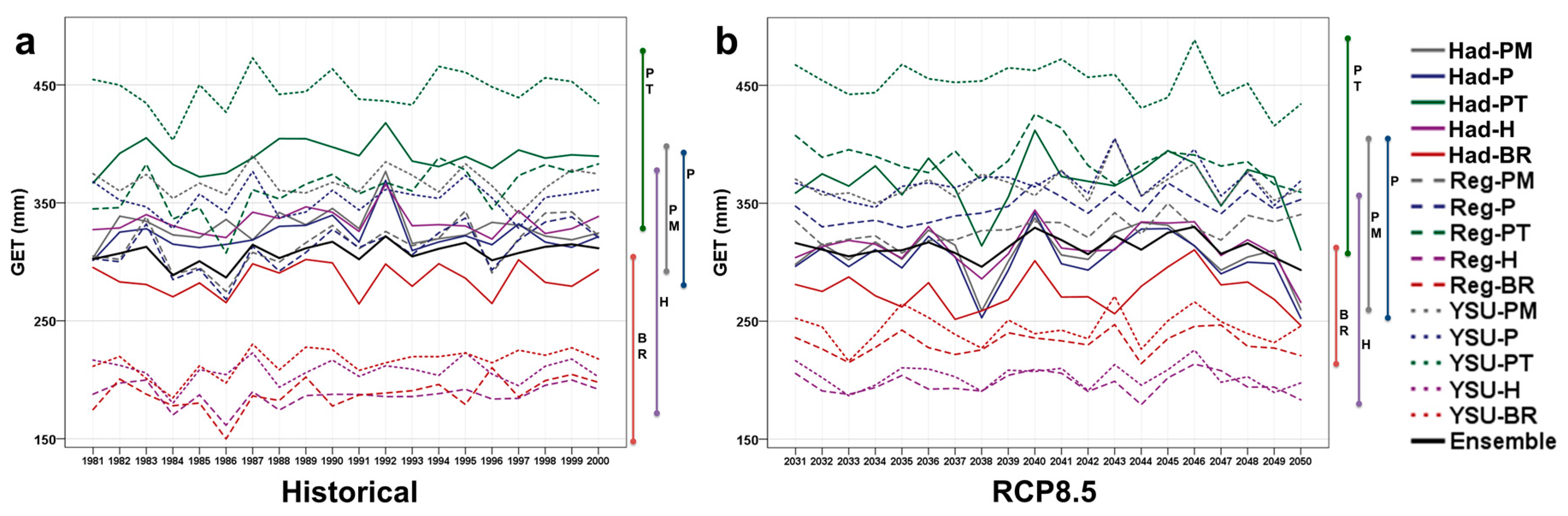
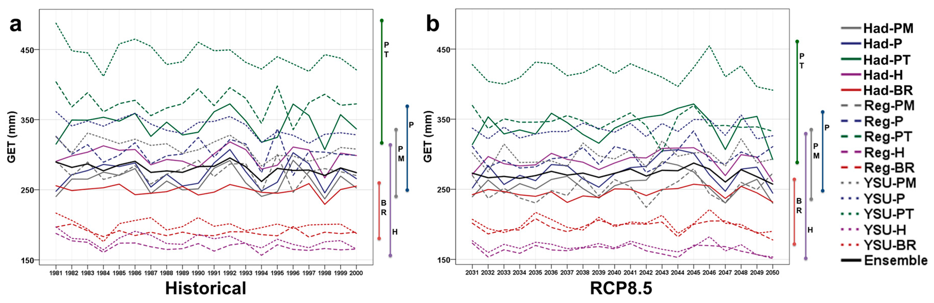
3.3. Estimation of Consumptive Water Use by Growing Season Evapotranspiration

The CWU was estimated using the growing season evapotranspiration (GET) data of each crop in the cropland. Similar to the PET estimation, three RCMs and five PET methods were applied, revealing fifteen results for the past and future periods. The GET estimation results differed largely from the RCM and PET method results, but the interval of the difference decreased as the total estimated amount decreased.

For the past data, the YSU-RSM-PT results (the most overestimated ones in PET) showed that the GET was 450 mm for both rice and maize, much higher than the other models. The RegCM4-BR results (the least underestimated PET results for rice) showed that the GET was less than 200 mm. The RegCM4-H results (least underestimated PET results for maize) showed that the GET was 165 mm on average. The average of the fifteen results was 307 mm for rice and 278 mm for maize (Figure 8 and Figure 9). Initially, the water consumption of rice was much higher, but the results for the two crops showed a small difference in average values due to the basic latitudinal differences in GET and the relatively long growing period in North Korea.

For the future period, the estimated GET of rice was generally similar to past values, and showed a slight increase with rising temperatures (Figure 8). From 2031 to 2050, the average of the ensemble values was 312 mm. The spatial pattern was the same as for the past values, but the values were slightly decreased (Figure 10). For maize, the pattern of the estimated values according to the RCM and PET methods was similar, but the overall GET value was slightly lower than the past values (Figure 9). This lower GET is caused by the shorter growing period in North Korea following the temperature increase. The ensemble value of the fifteen GETs of maize was 271 mm. The spatial distribution results also confirmed that the GET decreased significantly in North Korea (Figure 10).

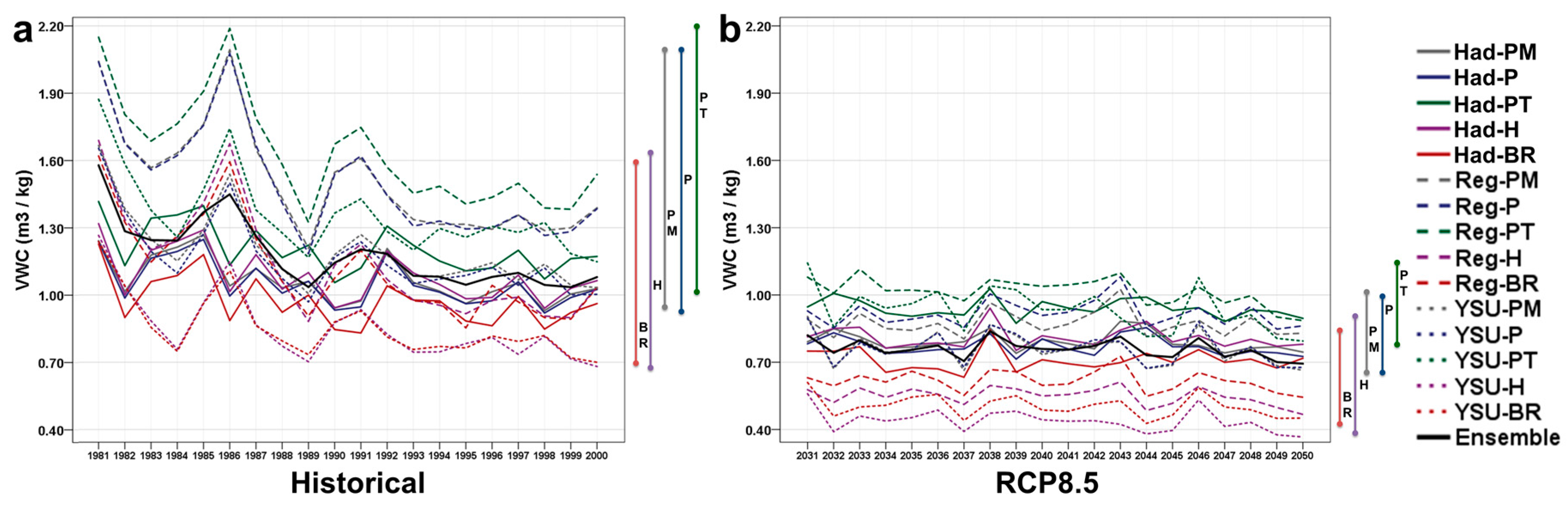
3.4. Virtual Water Content of Past and Future Using Multiple Data Sources

The crop yields and GET were used to calculate the VWC for each crop. Only the results from the three RCMs were estimated for the crop yield; therefore, the VWC was calculated using the five GETs and one crop yield, estimated by each RCM.

Reflected in the crop yield, the quantitative differences in the PET and the GET by the PET method significantly decreased. The VWC of rice ranged from 0.7 to 2.1 m³ kg⁻¹ and the average ensemble value was 1.18 m³ kg⁻¹, consistent with the past data (Figure 11). In the future estimates, the range decreases to 0.4~1.1 m³ kg⁻¹ and the mean value of the ensemble is 0.76 m³ kg⁻¹, significantly lower than the past data (Figure 11). These results indicate slight increases under the climate change scenario, but the rice yield is expected to increase greatly. The degree of change in the VWC calculated by the ratio of the two values is large. Spatially, there was a pattern of change similar to the rice yield result, with low VWC regions expanding northward (Figure 13).

The past values of the VWC of maize ranged between 0.3 and 1.0 m³ kg⁻¹, and the ensemble average was 0.58 m³ kg⁻¹ (Figure 12). Under the climate change scenario, the range decreased to 0.2–0.7 m³ kg⁻¹ and the ensemble average to 0.48 m³ kg⁻¹, slightly lower than the past values (Figure 12). Maize showed a smaller decrease in VWC than rice, and the maize yield is estimated to slightly increase while the GET slightly decreases. The degree of change in the VWC calculated by the ratio of the two values is relatively small. Spatial changes caused by climate change tend to be similar to the maize yield results, and the regions with lower VWCs are predicted to expand across the Korean Peninsula (Figure 13).

4. Discussion

4.1. Assessing the Ensemble Result of Crop Yield, PET, GET, and VWC

The four outputs (crop yield, PET, GET, and VWC) estimated in this study were calculated using multiple methods and multiple data sources, so the ensemble results presented here have a lower level of uncertainty. This ensemble approach is also emphasized in the future climate change research outlook [19,21].

One of the uncertainties addressed in this study is the uncertainty in crop yields in the climate data. Since crop yields have a high dependence on climate, the accuracy of the climate data is very important, even if the same crop model is used [17,53]. In this study, three RCM data sets were used, derived from one global climate model (GCM). The climate values calculated by each RCM are different from the previous studies, reflected in the crop yield results of this study [10,17]. Ultimately, three crop yields from each crop and period could be used to estimate a more realistic crop productivity for the Korean Peninsula.

There are many ways to estimate the evapotranspiration required for calculating VWC and to lower the uncertainty in the results of those methods [13,21]. The data required for the five PET methods used in this study were different, and the estimated results also showed great differences. The results of the H and BR methods, estimated using only the temperature, tend to be underestimated, and the results of the PT method, estimated using temperature and solar radiation, tend to be overestimated. Hence, the methodological uncertainty is lowered by the analysis of the differences in the methodologies and the ensemble result of evapotranspiration using multiple methodologies.

In particular, we calculated fifteen VWCs for each crop, which have inherent uncertainties due to the climate models and the PET method. Presenting the average of fifteen VWCs as an ensemble value resulted in mitigating the differences in data and methods by up to 294% (0.33–0.97 m³ kg⁻¹ (in 1986)) (historical maize data, annual average). The maximum difference of 252% (0.87–2.19 m³ kg⁻¹ (in 1986)) in the historical rice data was alleviated. In the future projections, the total VWC decreased compared to the past values, but the effect of the ensemble results was similar between the past and future values. The maximum reduction in the RCP85-rice value was 262% (0.42–1.10 m³ kg⁻¹ (in 2043)) and a reduction of up to 245% (0.31–0.76 m³ kg⁻¹ (in 2031)) was observed in RCP85-maize results (Figure 10 and Figure 11). In other words, the ensemble VWC reduced the difference by over 200% (according to data and methods) in all of the periods and crops. Although there are no VWC studies available for the Korean Peninsula, ensemble results are more similar than individual results when compared with the results of Zhao et al. [15], which calculated the VWC for China.

4.2. Implications for Agricultural Water Supply and Demand in the Korean Peninsula

Precipitation in the Korean Peninsula is concentrated in the summer monsoon season: 50–60% of annual precipitation occurs during this season. The water supply is not constant, as it is highly dependent on the river regime [10]. Most agricultural products in South Korea have been replaced by imported products due to changes at the economic level, but the self-sufficiency rate of food crops is so high that the consumption of water in agriculture is still at significant levels. In North Korea, the demand for water has increased because of the increase in food production owing to limited imports [24]. Overall, the Korean Peninsula, having a relatively high population density (South Korea: 519; North Korea: 208) and limited water supply, has a high demand for municipal, industrial, and agricultural water [55].

The average amount of water consumed by crops per unit production of major crops can be spatially determined by quantifying the agricultural water consumption using the results of the ensemble model approach employed in this study. This study also provided the future projections of the average agricultural water consumption, reflecting the impact of climate change, which has positive effects on productivity; as climate change accelerates, the amount of water consumed in the production of major crops will decrease. Climate change will have a negative impact on water supply as it affects precipitation patterns and amounts [10], but it can positively change water demand. However, this positive change in water demand due to climate change is the result of optimized adaptation modeling to water and nutrient stress. The consequences of climate change impacts without adaptation can vary significantly.

5. Conclusions

Multiple data sources and methods were employed in this study to estimate the past and future VWC of each crop in the Korean Peninsula. The EPIC crop model was used, and three RCMs and five PET methods were applied to reduce uncertainties in the data and methods. The rice and maize productivity varied significantly in the RCM results, confirming the increased potential production of both crops in the future. Positive changes in the northern part of the Korean Peninsula are noticeable, and maize is predicted to have high productivity in the entire peninsula in the future. The fifteen PETs and GETs from the RCM and PET methods were significantly different, and the water consumption of the crops was estimated by minimizing the errors by calculating the average values. The VWC was calculated for past and future crop yields and consumptive water use, with over 200% difference between them according to the RCM and PET methods. Computing the ensemble VWC for each period and crop by averaging fifteen VWCs could reduce the errors. The VWCs of the crops in the future projections were lower than those using the past data, which reflected a positive change in productivity and a decline in the length of the growth period. The past and future ensemble VWCs presented in this study provide quantitative data to shape the overall water demand for agriculture in the Korean Peninsula. We conclude that these results can be useful to improve agricultural sustainability, including food and water security, in the Korean Peninsula.

References

1. Sachs, J.D. From millennium development goals to sustainable development goals. Lancet 2012, 379, 2206–2211. [Google Scholar] [CrossRef]
2. IPCC. Climate Change 2014: Impacts, Adaptation, and Vulnerability. Part A: Global and Sectoral Aspects. Contribution of Working Group II to the Fifth Assessment Report of the Intergovernmental Panel on Climate Change; Cambridge University Press: Cambridge, UK, 2014. [Google Scholar]
3. Griggs, D.; Stafford-Smith, M.; Gaffney, O.; Rockström, J.; Öhman, M.C.; Shyamsundar, P.; Noble, I. Policy: Sustainable development goals for people and planet. Nature 2013, 495, 305–307. [Google Scholar] [CrossRef] [PubMed]
4. Wheeler, T.; Von Braun, J. Climate change impacts on global food security. Science 2013, 341, 508–513. [Google Scholar] [CrossRef] [PubMed]
5. Godfray, H.C.J.; Garnett, T. Food security and sustainable intensification. Philos. Trans. R. Soc. B 2004, 369, 20120273. [Google Scholar] [CrossRef] [PubMed]
6. Elliott, J.; Deryng, D.; Müller, C.; Frieler, K.; Konzmann, M.; Gerten, D.; Glotter, M.; Flörke, M.; Wada, Y.; Best, N.; et al. Constraints and potentials of future irrigation water availability on agricultural production under climate change. Proc. Natl. Acad. Sci. USA 2014, 111, 3239–3244. [Google Scholar] [CrossRef] [PubMed]
7. Calzadilla, A.; Rehdanz, K.; Betts, R.; Falloon, P.; Wiltshire, A.; Tol, R.S. Climate change impacts on global agriculture. Clim. Chang. 2013, 120, 357–374. [Google Scholar] [CrossRef]
8. Haddeland, I.; Heinke, J.; Biemans, H.; Eisner, S.; Flörke, M.; Hanasaki, N.; Stacke, T. Global water resources affected by human interventions and climate change. Proc. Natl. Acad. Sci. USA 2014, 111, 3251–3256. [Google Scholar] [CrossRef] [PubMed]
9. Huang, B.; Polanski, S.; Cubasch, U. Assessment of precipitation climatology in an ensemble of CORDEX-East Asia regional climate simulations. Clim. Res. 2015, 64, 141–158. [Google Scholar] [CrossRef]
10. Park, C.; Min, S.K.; Lee, D.; Cha, D.H.; Suh, M.S.; Kang, H.S.; Kwon, W.T. Evaluation of multiple regional climate models for summer climate extremes over East Asia. Clim. Dyn. 2016, 46, 2469–2486. [Google Scholar] [CrossRef]
11. Hoekstra, A.Y.; Hung, P.Q. Globalisation of water resources: International virtual water flows in relation to crop trade. Glob. Environ. Chang. 2005, 15, 45–56. [Google Scholar] [CrossRef]
12. Zhuo, L.; Mekonnen, M.M.; Hoekstra, A.Y. The effect of inter-annual variability of consumption, production, trade and climate on crop-related green and blue water footprints and inter-regional virtual water trade: A study for China (1978–2008). Water Res. 2016, 94, 73–85. [Google Scholar] [CrossRef] [PubMed]
13. Liu, J.; Zehnder, A.J.; Yang, H. Global consumptive water use for crop production: The importance of green water and virtual water. Water Resour. Res. 2009, 45. [Google Scholar] [CrossRef]
14. Liu, J.; Folberth, C.; Yang, H.; Röckström, J.; Abbaspour, K.; Zehnder, A.J. A global and spatially explicit assessment of climate change impacts on crop production and consumptive water use. PLoS ONE 2013, 8, e57750. [Google Scholar] [CrossRef] [PubMed]
15. Zhao, Q.; Liu, J.; Khabarov, N.; Obersteiner, M.; Westphal, M. Impacts of climate change on virtual water content of crops in China. Ecol. Inform. 2014, 19, 26–34. [Google Scholar] [CrossRef]
16. Zhuo, L.; Mekonnen, M.M.; Hoekstra, A.Y. Consumptive water footprint and virtual water trade scenarios for China—With a focus on crop production, consumption and trade. Environ. Int. 2016, 94, 211–223. [Google Scholar] [CrossRef] [PubMed]
17. Chun, J.A.; Li, S.; Wang, Q.; Lee, W.S.; Lee, E.J.; Horstmann, N.; Park, H.; Veasna, T.; Vanndy, L.; Pros, K.; et al. Assessing rice productivity and adaptation strategies for Southeast Asia under climate change through multi-scale crop modeling. Agric. Syst. 2016, 143, 14–21. [Google Scholar] [CrossRef]
18. Baek, H.-J.; Lee, J.; Lee, H.-S.; Hyun, Y.-K.; Cho, C.; Kwon, W.-T.; Marzin, C.; Gan, S.-Y.; Kim, M.-J.; Choi, D.-H. Climate change in the 21st century simulated by HadGEM2-AO under representative concentration pathways. Asia-Pac. J. Atmos. Sci. 2013, 49, 603–618. [Google Scholar] [CrossRef]
19. Rosenzweig, C.; Elliott, J.; Deryng, D.; Ruane, A.C.; Müller, C.; Arneth, A.; Boote, K.J.; Folberth, C.; Glotter, M.; Khabarov, N. Assessing agricultural risks of climate change in the 21st century in a global gridded crop model intercomparison. Proc. Natl. Acad. Sci. USA 2014, 111, 3268–3273. [Google Scholar] [CrossRef] [PubMed]
20. Wallach, D.; Rivington, M. A framework for assessing the uncertainty in crop model predictions. FACCE MACSUR Rep. 2014, 3, 1–5. [Google Scholar]
21. Liu, W.; Yang, H.; Folberth, C.; Wang, X.; Luo, Q.; Schulin, R. Global investigation of impacts of PET methods on simulating crop-water relations for maize. Agric. For. Meteorol. 2016, 221, 164–175. [Google Scholar] [CrossRef]
22. Choi, I.H.; Woo, J.C. Developmental process of forest policy direction in Korea and present status of forest desolation in North Korea. J. For. Sci. 2007, 23, 14. [Google Scholar]
23. Jeon, Y.; Kim, Y. Land reform, income redistribution, and agricultural production in Korea. Econ. Dev. Cult. Chang. 2000, 48, 253–268. [Google Scholar] [CrossRef]
24. Korea Rural Economic Institute (KREI). KREI Quarterly Agriculture Trends in North Korea; Korea Rural Economic Institute: Seoul, Korea, 2014. [Google Scholar]
25. Lee, J.W.; Hong, S.Y.; Chang, E.C.; Suh, M.S.; Kang, H.S. Assessment of future climate change over east Asia due to the RCP scenarios downscaled by GRIMs-RMP. Clim. Dyn. 2014, 42, 733–747. [Google Scholar] [CrossRef]
26. Giorgi, F.; Coppola, E.; Solmon, F.; Mariotti, L.; Sylla, M.B.; Bi, X.; Elguindi, N.; Diro, G.T.; Nari, V.; Giuliani, G.; et al. RegCM4: Model description and preliminary tests over multiple CORDEX domains. Clim. Res. 2012, 52, 7–29. [Google Scholar] [CrossRef]
27. Williams, J.R.; Jones, C.A.; Dyke, P.T. A modeling approach to determining the relationship between erosion and soil productivity. Trans. ASABE 1984, 27, 129–144. [Google Scholar] [CrossRef]
28. Williams, J.R.; Jones, C.A.; Kiniry, J.R.; Spanel, D.A. The EPIC crop growth model. Trans. ASAE 1989, 32, 497–511. [Google Scholar] [CrossRef]
29. Knisel, W.G. GLEAMS: Groundwater Loading Effects of Agricultural Management Systems 2006; Version 2.10 (No. 5); University of Georgia: Athens, GA, USA, 2006. [Google Scholar]
30. Izaurralde, R.; Williams, J.R.; McGill, W.B.; Rosenberg, N.J.; Jakas, M.Q. Simulating soil C dynamics with EPIC: Model description and testing against long-term data. Ecol. Model. 2006, 192, 362–384. [Google Scholar] [CrossRef]
31. Renard, K.G.; Foster, G.R.; Weesies, G.A.; Porter, J.P. Rusle: Revised Universal Soil Loss Equation. J. Soil Water Conserv. 1991, 46, 30–33. [Google Scholar]
32. Rinaldi, M. Application of EPIC model for irrigation scheduling of sunflower in Southern Italy. Agric. Water Manag. 2001, 49, 185–196. [Google Scholar] [CrossRef]
33. Williams, J.R. The EPIC model. In Computer Models of Watershed Hydrology; Singh, V.P., Ed.; Water Resources Publications: Littleton, CO, USA, 1995. [Google Scholar]
34. Xiong, W.; Balkovič, J.; van der Velde, M.; Zhang, X.; Izaurralde, R.C.; Skalský, R.; Lin, E.; Mueller, N.; Obersteiner, M. A calibration procedure to improve global rice yield simulations with EPIC. Ecol. Model. 2014, 273, 128–139. [Google Scholar] [CrossRef]
35. Lim, C.H.; Lee, W.K.; Song, Y.; Eom, K.C. Assessing the EPIC model for estimation of future crops yield in South Korea. J. Clim. Chang. Res. 2015, 6, 21–31. [Google Scholar] [CrossRef]
36. Lim, C.H.; Kim, M.; Lee, W.K.; Folberth, C. Spatially Explicit Assessment of Agricultural Water Equilibrium in the Korean Peninsula. Agric. Water Manag. 2017. under review. [Google Scholar]
37. Balkovič, J.; van der Velde, M.; Schmid, E.; Skalský, R.; Khabarov, N.; Obersteiner, M.; Xiong, W. Pan-European crop modelling with EPIC: Implementation, up-scaling and regional crop yield validation. Agric. Syst. 2013, 120, 61–75. [Google Scholar] [CrossRef]
38. Lim, C.H.; Choi, Y.; Kim, M.; Jeon, S.W.; Lee, W.K. Impact of deforestation on agro-environmental variables in cropland, North Korea. Sustainability 2017. under review. [Google Scholar]
39. Yoo, B.H.; Kim, K.S. Development of a gridded climate data tool for the Coordinated Regional climate Downscaling Experiment data. Comput. Electron. Agric. 2017, 133, 128–140. [Google Scholar] [CrossRef]
40. Nash, J.E.; Sutcliffe, J.V. River flow forecasting through conceptual models part I—A discussion of principles. J. Hydrol. 1970, 10, 282–290. [Google Scholar] [CrossRef]
41. Niu, X.; Easterling, W.; Hays, C.J.; Jacobs, A.; Mearns, L. Reliability and input-data induced uncertainty of the EPIC model to estimate climate change impact on sorghum yields in the US Great Plains. Agric. Ecosyst. Environ. 2009, 129, 268–276. [Google Scholar] [CrossRef]
42. Balkovič, J.; van der Velde, M.; Skalský, R.; Xiong, W.; Folberth, C.; Khabarov, N.; Smirnov, A.; Mueller, N.D.; Obersteiner, M. Global wheat production potentials and management flexibility under the representative concentration pathways. Glob. Planet. Chang. 2014, 122, 107–121. [Google Scholar] [CrossRef]
43. Monteith, J. Evaporation and environment. Symp. Soc. Exp. Biol. 1965, 19, 205–234. [Google Scholar] [PubMed]
44. Penman, H.L. Natural evaporation from open water, bare soil and grass. Proc. R. Soc. Lond. Ser. A 1948, 193, 120–145. [Google Scholar] [CrossRef]
45. Priestley, C.; Taylor, R. On the assessment of surface heat flux and evaporation using large-scale parameters. Mon. Weather Rev. 1972, 100, 81–92. [Google Scholar] [CrossRef]
46. Hargreaves, G.H.; Samani, Z.A. Reference crop evapotranspiration from temperature. Appl. Eng. Agric. 1985, 1, 96–99. [Google Scholar] [CrossRef]
47. Baier, W.; Robertson, G.W. Estimation of latent evaporation from simple weather observations. Can. J. Plant Sci. 1965, 45, 276–284. [Google Scholar] [CrossRef]
48. Liu, J.; Williams, J.R.; Zehnder, A.J.; Yang, H. GEPIC—Modelling wheat yield and crop water productivity with high resolution on a global scale. Agric. Syst. 2007, 94, 478–493. [Google Scholar] [CrossRef]
49. Food Agriculture Organization. FAO Digital Soil Map of the World; FAO: Rome, Italy, 1995. [Google Scholar]
50. Batjes, N.H. ISRIC-WISE Derived Soil Properties on a 5 by 5 Arc-Minutes Global Grid; ISRIC—World Soil Information: Wageningen, The Netherlands, 2006. [Google Scholar]
51. Chen, J.; Chen, J.; Liao, A.; Cao, X.; Chen, L.; Chen, X.; Zhang, W. Global land cover mapping at 30 m resolution: A POK-based operational approach. ISPRS J. Photogramm. Remote Sens. 2015, 103, 7–27. [Google Scholar] [CrossRef]
52. Kim, H.Y.; Ko, J.; Kang, S.; Tenhunen, J. Impacts of climate change on paddy rice yield in a temperate climate. Glob. Chang. Biol. 2013, 19, 548–562. [Google Scholar] [CrossRef] [PubMed]
53. Shin, Y.; Lee, E.J.; Im, E.S.; Jung, I.W. Spatially distinct response of rice yield to autonomous adaptation under the CMIP5 multi-model projections. Asia-Pac. J. Atmos. Sci. 2017, 53, 21–30. [Google Scholar] [CrossRef]
54. Liaqat, U.W.; Choi, M. Accuracy comparison of remotely sensed evapotranspiration products and their associated water stress footprints under different land cover types in Korean peninsula. J. Clean. Prod. 2017, 155, 93–104. [Google Scholar] [CrossRef]
55. Chung, E.S.; Won, K.; Kim, Y.; Lee, H. Water resource vulnerability characteristics by district’s population size in a changing climate using subjective and objective weights. Sustainability 2014, 6, 6141–6157. [Google Scholar] [CrossRef]
Figure 1. Land cover map of the research area.
Sustainability 09 01172 g001
Figure 2. Schematic diagram of the applied methodology. RCM, regional climate model; PET, potential evapotranspiration; VWC, virtual water content; growing season evapotranspiration (GET).
Sustainability 09 01172 g002
Figure 3. Estimated crop yield using multiple regional climate models (RCMs) in the past and future (a) Historical-rice; (b) representative concentration pathways (RCP) 8.5-rice; (c) Historical-maize; (d) RCP8.5-maize.
Sustainability 09 01172 g003
Figure 4. Spatial distribution of rice yield in the past and future for each climate model.
Sustainability 09 01172 g004
Figure 5. Spatial distribution of maize yield in the past and future for each climate model.
Sustainability 09 01172 g005
Figure 6. Estimated PET using multiple RCMs and PET methods for the past and future (a) Historical period (1981–2000); (b) RCP8.5 scenario (2031–2050).
Sustainability 09 01172 g006
Figure 7. Spatial distribution of potential evapotranspiration for the past and future using the ensemble result.
Sustainability 09 01172 g007
Figure 8. Estimated GET of rice using multiple RCMs and PET methods in the past and future (a) Historical period (1981–2000); (b) RCP8.5 scenario (2031–2050).
Sustainability 09 01172 g008
Figure 9. Estimated GET of maize using multiple RCMs and PET methods in the past and future (a) Historical period (1981–2000); (b) RCP8.5 scenario (2031–2050).
Sustainability 09 01172 g009
Figure 10. Spatial distribution of growing season evapotranspiration in the past and future using the ensemble result.
Sustainability 09 01172 g010
Figure 11. Estimated VWC of rice using multiple RCMs and PET methods in past and future (a) Historical period (1981−2000); (b) RCP8.5 scenario (2031−2050).
Sustainability 09 01172 g011
Figure 12. Estimated VWC of maize using multiple RCMs and PET methods in the past and the future (a) Historical period (1981−2000); (b) RCP8.5 scenario (2031−2050).
Sustainability 09 01172 g012
Figure 13. Spatial distribution of virtual water contents of crops in the past and future using the ensemble result.
Sustainability 09 01172 g013